If one considers partitioning the spanning trees of a weighted graph into weight classes, a number of ... validity of each of these statements follows easily from the proof of correctness of. Kruskal's .... Proof: We prove the contrapositive. Accordingly ..... On the shortest spanning subtree of a graph and the traveling salesman ...
On the Spanning Trees of Weighted Graphs� Ernst W. Mayr
C. Greg Plaxton
y
Abstract Given a weighted graph, let W1 ; W2; W3; : : : denote the increasing sequence of all possible distinct spanning tree weights. Settling a conjecture due to Kano, we prove that every spanning tree of weight W1 is at most k ? 1 edge swaps away from some spanning tree of weight Wk . Three other conjectures posed by Kano are proven for two special classes of graphs. Finally, we consider the algorithmic complexity of generating a spanning tree of weight Wk .
1 Introduction The minimum spanning tree problem is a classic problem in computer science for which a large number of sequential, parallel and distributed algorithms have been devised. To the graph theorist, however, this body of work has provided little beyond the underlying proof of correctness of the original greedy algorithms due to Kruskal and Prim [Kr][Pr]. Evidently, the advances have occurred in the areas of data structures, parallel processing techniques and distributed protocols. In contrast, this paper attacks questions arising from a generalization of the minimum spanning tree concept that requires additional insight at the graph-theoretic level. If one considers partitioning the spanning trees of a weighted graph into weight classes, a number of natural questions arise with regard to relationships between the classes. In a recent paper, Kano [Kan] posed four conjectures that were motivated by the previous work of Kawamoto, Kajitani and Shinoda [KKS]. Our main result is a proof that every minimum spanning tree is at most k ? 1 edge swaps away from some representative of the kth weight class, settling the rst of Kano's conjectures. With regard to the three remaining conjectures, we o�er a stronger uni ed conjecture and prove that it holds for two non-trivial families of graphs. We also consider the algorithmic complexity of generating a representative of the kth weight class. For xed k, we obtain a polynomial time algorithm. When k is part This work was supported in part by a grant from the AT&T Foundation and NSF grant DCR8351757. y Primarily supported by a 1967 Science and Engineering Scholarship from the Natural Sciences and Engineering Research Council of Canada. �
of the input, the associated decision problem (KMST) is seen to be NP-hard using a reduction due to Johnson and Kashdan [JK] for the related kth best spanning tree problem (KBST). Lawler [La] gave a simple branch-and-bound algorithm for KBST with a running time that is pseudo-polynomial in k. The existence of such an algorithm provides a hopeful sign that a similar result might be possible for KMST. We do not achieve this goal, but by extending a determinant method due to Okada and Onodera [OO], we obtain an algorithm for which the running time is pseudo-polynomial in the edge weights as well as k.
2 Preliminaries Let G = (V; E ) be a connected undirected graph with a real-valued weight w(e) assigned to each edge e 2 E . Let e? and e denote the endpoints of edge e. Parallel edges and self-loops are permissible. For any subset E 0 of E de ne the weight of E 0, denoted w(E 0), as the sum of the weights of the edges of E 0, that is, X w(E 0) = w(e): +
e2E 0
A spanning tree P of G is any subset of E for which the graph (V; P ) is acyclic and connected; in order to satisfy both of these properties simultaneously it is necessary that jP j = jV j ? 1. In order to discuss the partition of the spanning trees of G into weight classes, we will make use of the following notation. T (G) = fP j P is a spanning tree of Gg W (G) = fx j w(P ) = x for some P 2 T (G)g N (G) = jW (G)j Wi(G) = the ith smallest element of W (G); 1 � i � N (G) Ti(G) = fP 2 T (G) j w(P ) = Wi(G)g �(G; P ) = i; if and only if P 2 Ti(G) �(G; P ) = jTi(G)j; if and only if P 2 Ti(G) A spanning tree of weight W (G) is a minimum spanning tree of G. In general, a spanning tree of weight Wk (G) will be referred to as a kth minimal spanning tree (kMST) of G. Note that some previous authors have preferred to formulate their results in terms of kth maximal spanning trees [Kan][KKS], an equivalent concept. Let P and Q be spanning trees of G. Then jP n Qj is the distance between P and Q and will be denoted by d(P; Q). For any nonnegative integer k, let Lk (G; P ) represent the set of all spanning trees Q of G such that d(P; Q) � k. Notice that d(P; Q) = d(Q; P ) so that Q 2 Lk (G; P ) if and only if P 2 Lk (G; Q). For every e 62 P , let Cyc (P; e) denote the fundamental cycle of G de ned by e with respect to P . Given distinct edges a; b such that a 2 Cyc (P; b), the spanning tree P n fag [ fbg is de ned to be a single edge swap away from P . For any two spanning trees P and Q, we note that the length of the shortest sequence of edge swaps required to transform P into Q is precisely d(P; Q). 1
2
We will have occasion to make use of several well-known facts about 1-MSTs. The validity of each of these statements follows easily from the proof of correctness of Kruskal's greedy algorithm for computing a 1-MST [Kr].
Fact 1 A spanning tree is a 1-MST of G if and only if it is a 1-MST in L (G; P ). 1
Fact 2 The unique heaviest edge in some cycle cannot belong to any 1-MST. A heaviest
edge in some cycle cannot belong to every 1-MST.
Fact 3 The unique lightest edge in some cutset must belong to every 1-MST. A lightest edge in some cutset must belong to some 1-MST.
Fact 4 Every 1-MST contains the same distribution of edge weights. Fact 5 Every 1-MST can be generated by Kruskal's algorithm. Given Fact 1, it is straightforward to verify that for any i-MST P of G, Li? (G; P ) contains a 1-MST. However, going in the other direction turns out to be much more di�cult. Kawamoto, Kajitani and Shinoda [KKS] studied 2-MSTs and proved that for every 1-MST P there is a 2-MST Q such that d(P; Q) = 1. This led Kano to pose the following conjecture, for which the result of Kawamoto et al. corresponds to the special case i = 2. 1
Conjecture 1 If P is a 1-MST of G then Li? (G; P ) contains an i-MST, 1 � i � 1
N (G).
Kano was able to prove that Conjecture 1 holds for i = 3 and 4. We will show that Conjecture 1 is, indeed, a theorem. Kano also proposed the following three conjectures, proving them for values of i less than or equal to 3, 4 and 3, respectively.
Conjecture 2 If P is an i-MST in Li(G; P ) then P is an i-MST of G. Conjecture 3 If P is an i-MST of G then P is an i-MST in Li? (G; P ). 1
Conjecture 4 Let ?(i; j ) denote the graph with vertex set Ti(G) and an edge between each pair of i-MSTs P; Q such that d(P; Q) � j . Then ?(i; i) is connected.
3 Proofs In this section, we prove Conjecture 1 along with a number of other results.
Lemma 3.1 Let P and Q be spanning trees of a given graph G. Then for each edge p 2 P n Q there is an edge q 2 Q n P such that p 2 Cyc (P; q) and q 2 Cyc (Q; p). 3
Proof: Let P , Q and p be as de ned above and assume that there is no edge q satisfying the requirements of the lemma. Then there must be a path made up of edges from P n fpg that connects the two endpoints of p. But then P contains a cycle, contradicting the assumption that it is a spanning tree.
De nition 3.1 Given a graph G = (V; E ), let � represent G or any subset of E . If
C and D are disjoint subsets of E , then the graph or set of edges produced from � by contracting the edges of C and discarding the edges of D will be denoted �[C; D]. Notice that there is a 1-1 correspondence between the edges of �[C; D] and those edges of � that do not belong to C [ D. We identify the pairs of edges determined by this correspondence, inheriting edge weights in the weighted case.
We note that if P is a spanning tree of G, then P [c; d] is a spanning tree of G[c; d] if and only if c 2 P and d 62 P , or c 62 P and d 2 Cyc (P; c).
Lemma 3.2 Let P be a spanning trees of a weighted graph G = (V; E ). For any edge e 62 P , let G0 = G[; e] and P 0 = P . For any edge e 2 P , let G0 = G[e; ] and P 0 = P [e; ].
In either case, the following statements hold: 1. P 0 is a spanning tree of G0 . 2. �(G0 ; P 0) � �(G; P ).
3. �(G0 ; P 0) � �(G; P ).
Proof: The above statements follow easily once we exhibit an injective map � from T (G0) to T (G) that takes P 0 to P and also satis es a \constant displacement" property, namely, there exists a real value � such that for all spanning trees R0 2 T (G0), w(�(R0 )) = w(R0 ) + �: (1) For the case e 62 P , take �(R0) to be simply R0 so that equation 1 holds with � = 0. For e 2 P , let �(R0 ) be the unique spanning tree R 2 T (G) such that R[e; ] = R0 and set � = w(e).
Lemma 3.3 Let P be a 1-MST of a given weighted graph G = (V; E ). For any edge e 2 P , let P 0 = P [e; ]. For any edge e 62 P , let P 0 = P [e; h] where h is a heaviest edge on Cyc (P; e) n feg. In either case, P 0 is a 1-MST of G[e; ]. Proof: If e 2 P then Lemma 3.2 applies. Assume that e 62 P . Appealing to Fact 5,
consider an execution of Kruskal's algorithm on input G that generates the 1-MST P . As each edge p 2 P gets added to P , Kruskal's algorithm running on input G[e; ] can correctly select p with one exception: the edge that rst puts e? and e into the same component must be omitted. This edge must have weight w(h) since it is a heaviest edge on the path from e? to e in P . +
+
4
De nition 3.2 A graph G = (V; E ) will be called a bispanning graph if E is the union
of two disjoint spanning trees P and Q. Such a bispanning graph will be denoted by the triple (V; P; Q).
De nition 3.3 A simple bispanning graph is a bispanning graph that contains only cycles of length 2.
The following result was obtained previously by Kano using Hall's Theorem [Kan]. Here we provide an alternative proof that is explicitly constructive and introduces some of the ideas that will be used to prove Conjecture 1.
Theorem 1 Let P be a 1-MST and Q be an arbitrary spanning tree of a given weighted graph G = (V; E ). Then there exists a bijection � from P n Q to Q n P such that for every edge e 2 P n Q, �(e) 2 Cyc (Q; e) and w(�(e)) � w(e). Proof: It is su�cient to determine a bijection between the disjoint spanning trees P 0 = P n Q and Q0 = Q n P of the bispanning graph G0 = G[P \ Q; E n P n Q]. This is due to the observation that Cyc (Q0; e) � Cyc (Q; e) for all e 2 P 0. Let p be a heaviest edge in P 0 and let q be any edge in Q0 for which p 2 Cyc (P 0; q) and q 2 Cyc (Q0; p). Lemma 3.1 guarantees that we can nd such a q. As P 0 is a 1-MST, we must have w(Q) � w(P ). Let �(p) = q.
To determine the next component of the bijection, repeat this procedure on the bispanning graph G0[q; p] with disjoint spanning trees P 0[q; p] and Q0[q; p]. P 0[q; p] is a 1-MST of G0[q; p] by Lemma 3.3. Furthermore, for all e 2 P 0[q; p], Cyc (Q0[q; p]; e) = Cyc (Q0; e) n fqg � Cyc (Q0; e) � Cyc (Q; e)
so that subsequent assignments to � will be guaranteed to satisfy the condition �(�) 2 Cyc (Q; �).
Lemma 3.4 Conjecture 1 holds if and only if there is no weighted bispanning graph B = (V; P; Q) such that d(P; Q) � �(B; Q) > �(B; P ) = 1 and �(B; Q) = 1. Proof: The \only if" directon is easy. To establish the \if" direction, we will prove
the contrapositive. Given a counterexample (G; P; i) to Conjecture 1, let Q be a closest i-MST to P . Then repeated application of Lemma 3.2 proves that the bispanning graph G0 = G[P \ Q; E n P n Q] with disjoint spanning trees P 0 = P n Q and Q0 = Q n P also violates the conjecture, that is, d(P 0; Q0) � �(G0; Q0) > �(G0; P 0) = 1. It remains to be proven that �(G0; Q0) = 1. If not, there must be a spanning tree Q00 of G0 such that w(Q00) = w(Q0) and Q00 6= Q0. Then d(P 0; Q00) � d(P 0; Q0) by the de nition of Q. On the other hand, d(P 0; Q00) < d(P 0; Q0) since Q00 must have at least one edge in common with P 0, whereas Q0 has none. Thus, Q0 must have unique weight in T (G0), as required. 5
Theorem 2 There is no weighted bispanning graph B = (V; P; Q) such that d(P; Q) � �(B; Q) > �(B; P ) = 1 and �(B; Q) = 1. Hence, Conjecture 1 holds by Lemma 3.4.
Proof: Assume the theorem is false and let B = (V; P; Q) be a counterexample with smallest possible jV j. We will establish a contradiction by exhibiting a smaller
counterexample B 0. As in the proof of Theorem 1, let p be a heaviest edge in P and let q be any edge in Q for which p 2 Cyc (P; q) and q 2 Cyc(Q; p). Since P is a 1-MST and �(B; Q) = 1, we must have w(Q) > w(P ). Therefore, q is the unique heaviest edge in Cyc (P; q) and does not belong to any 1-MST of B by Fact 2. Now consider the smaller bispanning graph B 0 = B [q; p] with disjoint spanning trees P 0 = P [q; p] and Q0 = Q[q; p]. Clearly, d(P 0; Q0) = d(P; Q) ? 1. Furthermore, �(B 0; P 0) = 1 and �(B 0; Q0) = 1 by Lemmas 3.3 and 3.2, respectively. In order to show that B 0 is a counterexample to the theorem, it is su�cient to prove that �(B 0; Q0) < �(B; Q). Lemma 3.2 gives us only �(B 0; Q0) � �(B; Q), but in the present case that argument can be strengthened to yield the desired strict inequality. Namely, let � be the injective map taking R0 2 T (B 0) to R 2 T (B ) such that R0 = R[q; p] and observe that � does not map any spanning tree of B 0 into T (B ). The statements proven by the next three lemmas all have the structure of Lemma 3.4, underscoring the similarities between Kano's various conjectures. Note, however, that Lemma 3.5 is proven in one direction only. 1
Lemma 3.5 Conjecture 2 holds if there is no weighted bispanning graph B = (V; P; Q) such that d(P; Q) � �(B; Q) > �(B; P ) and �(B; Q) = 1. Proof: We prove the contrapositive. Accordingly, let (G; R; i) be a counterexample to Conjecture 2, that is, R is an i-MST in Li(G; R) but not an i-MST of G. There must be a least integer j < i such that Li(G; R) does not contain a j -MST. By Fact 1, there must be a k-MST P such that d(P; R) � i ? k for some k < j . Let Q be a closest j -MST to P . Since Q is not contained in Li (G; R) we have
d(P; Q) � i ? d(P; R) � k: Now consider the bispanning graph G0 = G[P \ Q; E n P n Q] with disjoint spanning trees P 0 = P n Q and Q0 = Q n P . By repeated application of Lemma 3.2,
d(P 0; Q0) � �(G0; Q0) > �(G0 ; P 0) and �(G0; Q0) = 1 so the proof is complete.
Lemma 3.6 Conjecture 3 holds if and only if there is no weighted bispanning graph B = (V; P; Q) such that d(P; Q) � �(B; P ) > �(B; Q) and �(B; Q) = 1. 6
Proof: The proof is similar to that given for Lemma 3.4. In this case, assume that (G; P; i) is a counterexample to Conjecture 3, let j be any integer less than i such that Li? (G; P ) does not contain a j -MST, and let Q be a closest j -MST to P . 1
Lemma 3.7 Conjecture 4 holds if and only if there is no weighted bispanning graph
B = (V; P; Q) such that d(P; Q) > �(B; P ) = �(B; Q) and �(B; Q) = 2.
Proof: Once again, the proof is similar to that given for Lemma 3.4. Assume that
(G; i) is a counterexample to Conjecture 4, and let P; Q be a closest pair of i-MSTs belonging to di�erent connected components of ?(i; i). Given a weighted bispanning graph B = (V; P; Q) such that Q has unique weight in T (B ) n fP g, let i = �(B; P ), j = �(B; Q), a = maxfi; j g and b = minfi; j g. Unifying the \if" statements of Lemmas 3.4 through 3.7, we nd that all of Kano's conjectures hold if we can guarantee that d(P; Q) � maxfa ? 1; bg. This bound does not appear to be attainable for all values of a and b. We expect that it can be strengthened to the inequality stated below. Conjecture 5 Let P; Q; a; b be as de ned in the preceding paragraph. Then 8 > if a = b; < a; d(P; Q) � > aj ? 1; k if a > b = 1; : a b? ; otherwise. + 1 2
This conjecture is strongest possible if a ? b is odd, a = b or b = 1, as may be easily seen by assigning appropriate edge weights to simple bispanning graphs. Furthermore, Conjecture 5 implies the following bound for general graphs that is optimal in the sense that equality can be achieved for all values of a and b. Lemma 3.8 Let P be an i-MST of a given weighted graph G and suppose that Q is a closest j -MST to P in T (G)nfP g. Let a = maxfi; j g and b = minfi; j g. If Conjecture 5 holds, then ( a; if a = b; d(P; Q) � max na ? b; j a b? ko ; otherwise. + 1 2
Proof: Apply Lemma 3.2 until the bispanning graph G[P \ Q; E n P n Q] is obtained,
then use Conjecture 5. Thus far, we have been able to prove Conjecture 5 only for certain special classes of graphs. We will now examine two such families that were obtained by restricting: the graph structure, in the rst case, and the set of allowable edge weights, in the second case.
De nition 3.4 Let P and Q be spanning trees of a given graph G. Then P and
Q are related by a parallel swap if and only if there exists a bijection � from P n Q = fe ; : : : ; etg to Q n P = f�(e ); : : : ; �(et)g such that each of the 2t sets of jP j edges containing P \ Q and exactly one edge from each pair fei; �(ei)g; 1 � i � t, is a spanning tree of G. 1
1
7
u
@
?
@ ?
@ ? ? @
u
? @
?
u
@u
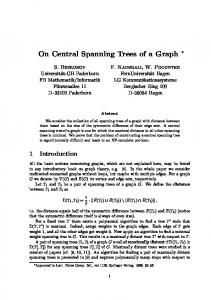
Figure 1: The smallest bispanning graph without a parallel swap. As an aside, it is possible to prove that spanning trees P and Q are related by a parallel swap if and only if Lemma 3.1 is satis ed by a unique q 2 Q n P for each p 2 P n Q. This means that one may readily determine whether or not two particular spanning trees are related by a parallel swap.
Theorem 3 Let B = (V; P; Q) be a bispanning graph for which P and Q are related by a parallel swap. Then Conjecture 5 holds.
Proof: Let B be a counterexample with smallest possible jV j. Without loss of
generality, we can assume that B is a simple bispanning graph. Observe that for all R 2 T (B ), R = E n R also belongs to T (B ) and �(B; R) + �(B; R) = N (B ) + 1. Hence, P has unique weight in T (B ) n fQg. If either P or Q is a 1-MST then the result follows easily by Fact 1. If w(P ) = w(Q) then contract any cycle to obtain a smaller counterexample. If two possible edge swaps increase (decrease) the weight of P by di�erent amounts, then contract the cycle corresponding to the larger change in order to obtain a smaller counterexample. The preceding argument allows us to assume that s of the possible edge swaps in B increase the weight of P by some amount � while each of the remaining jV j? 1 ? s edge swaps causes a decrease of � . It is straightforward to prove that a weighted bispanning graph of this form cannot provide a counterexample to Conjecture 5. If Conjecture 5 holds for all bispanning graphs with up to n vertices, then Conjectures 2, 3 and 4 must hold for all values of i less than or equal to n ? 1, n and n ? 1, respectively. It is easy to check that every bispanning graph B = (V; P; Q) with jV j � 3 admits a parallel swap between P and Q. For jV j = 4, only the bispanning graph in Figure 1 does not have this property, but we can show by case analysis that Conjecture 5 holds for this particular graph as well. These observations re-establish the results obtained by Kano with respect to the small cases of Conjectures 2 through 4. Another interesting class of weighted graphs for which we can prove Conjecture 5 are those with edge weights drawn from an arithmetic sequence of length 3. Weighted graphs of this sort arise in the analysis of LCR networks [Kaj], and Kano was able to prove Conjecture 1 for such graphs. 1
2
8
Theorem 4 Let B = (V; P; Q) be a weighted bispanning graph with edge weights drawn from the set fa; a + d; a + 2dg. Then Conjecture 5 holds. Proof Sketch: Assume without loss of generality that a = 0 and d = 1, and let B = (V; P; Q) be a counterexample with smallest possible jV j. We will brie y outline the proof of the hardest case, which turns out to occur when W (Q) > W (P ) > W (B ). Let Q0 be a lightest spanning tree in L (Q). Either W (Q0) = W (Q) ? 1 or W (Q0) = W (Q) ? 2. If W (Q0) = W (Q) ? 1, it is possible to prove that �(B; Q) > 1, a contradiction. If W (Q0) = W (Q) ? 2 then we show that P must be a 2-MST with W (P ) = W (B ) + 1 or else �(B; Q) > 1. It is now su�cient to prove that there is an edge q 2 Q of weight 2 such that Cyc (P; q) contains an edge p of weight 0, since this implies the existence of a smaller counterexample B [q; p]. 1
1
1
4 The Generation Problem For xed k, Theorem 2 yields a polynomial time algorithm for computing a k-MST. In particular, if n = jV j and m = jE j we have
Corollary 4.1 Given a weighted graph G, a k-MST of G can be generated in O((mn)k? ) time. 1
Proof: First compute a 1-MST M . This can be done in O(m + n log n) time using
Fibonacci heaps [FT], although for the present argument it would su�ce to use one of the simpler 1-MST algorithms with a higher asymptotic running time. Then compute the weight of all spanning trees that are strictly fewer than k edge swaps away from M . There are at most kX ? n ? 1! m ? n + 1 ! = O((mn)k? ) (2) i i i such spanning trees and the weight of each tree can be computed incrementally in constant time by performing the enumeration in a depth- rst manner. At any point in the computation we need to remember the k largest distinct weights found so far. This only increases the running time by a constant factor since k is xed. In order to discuss complexity issues, we introduce the language problem associated with the problem of nding a k-MST. 1
1
=0
De nition 4.1 Given a graph G = (V; E ), positive integer weights w(e) for each e 2 E , positive integers k and B . The KMST problem is to determine whether or not there are k spanning trees of G with distinct weights less than or equal to B .
By omitting the word \distinct" from De nition 4.1, we get the de nition of the kth best spanning tree problem (KBST). 9
Theorem 5 KMST is NP-hard. Proof: The proof is identical to the one given in [JK] for KBST, which is not known
to be in NP. The reduction is from HAMILTON CIRCUIT. Note that the O((mn)k? ) algorithm described earlier does not solve KMST in time pseudo-polynomial in k. The running time of such an algorithm would have to be polynomial in jV j, k, log B and log wmax , where wmax is the weight of the heaviest edge. Interestingly, a pseudo-polynomial time solution is known for KBST; the approach is to generate all spanning trees up to the kth [La]. Unfortunately, this method is not powerful enough for KMST since there may be exponentially many spanning trees belonging to classes below the kth. We will now present a determinant-based KMST algorithm for which the running time is pseudo-polynomial in the edge weights as well as k. Let G be a graph with n + 1 vertices v ; : : :; vn and m edges e ; : : :; em. Construct the m � (n + 1) matrix A with 8 > +1; if ei = (vj ; vk ) for some k > j ; < aij = > ?1; if ei = (vj ; vk ) for some k < j ; : 0; otherwise. 1
0
1
and let A be the m � n matrix A with column 0 deleted. Letting AS denote the matrix (aij ) for i 2 S and j ranging from 1 to n, we have X det AT A = [det AS ] 0
0
0
2
S�f1;:::;mg jSj=n
by the Binet-Cauchy formula (see [Kn]). Furthermore, ( 1; if (V; S ) is a tree; det AS = � 0; otherwise.
(3)
so that the determinant of AT A is the number of spanning trees of G. This result is due to Okada and Onodera [OO]. Similary, we can construct the m � (n + 1) matrix B with 8 w ei > < +xw e ; if ei = (vj ; vk) for some k > j ; bij = > ?x i ; if ei = (vj ; vk) for some k < j ; : 0; otherwise. 0
0
(
)
(
)
and let B be the m � n matrix A with column 0 deleted. Let p(x) be the determinant of B T A , and let pk be the coe�cient of xk in p(x). h i det B T A = det (xw e1 � � � xw em )AT A X = [det AS ] xw S 0
0
0
0
(
0
)
(
2
=
S�f1;:::;mg jSj=n
X
pk xk
10
)
( )
0
0
Using equation 3 we nd that pk is the number of spanning trees of G with weight k, that is, p(x) is the generating function for the number of spanning trees in each weight class of G. This relationship leads us to a pair of algorithms for solving KMST. The rst idea is to compute det B T A for all integer values of x from 0 up to Wmax , where Wmax = WN G (G), and then interpolate to obtain p(x). The interpolation is the most costly step, and it involves solving a system of Wmax + 1 equations with O(Wmax ) digit integer coe�cients. This can be done in time polynomial in Wmax by the result of Edmonds [Ed], who proved that Gaussian elimination with pivoting is in P for exact rational arithmetic. A second approach is to obtain an upper bound for pk and then compute det B T A for a single value of x that is large (or small) enough to ensure that all of the coe�cients pk can be extracted from the nal result. Letting C = B T A with x = 1, we can derive a suitable bound on pk as follows. 0
0
( )
2
0
0
pk � det C 0 Y @X
�
�i�n
1
�j �n
1
0
0
1= cij A
1 2
2
The rst inequality follows from the fact that pk � 0 for all k; the second is Hadamard's inequality. Either of these methods gives a KMST algorithm with running time pseudo-polynomial in the edge weights as well as k. At the expense of an extra polynomial factor, we can easily convert them into algorithms for generating a k-MST.
5 Open Problems We have succeeded in proving one of Kano's four conjectures; the remaining three would be established by a proof of Conjecture 5. The existence of a pseudo-polynomial (in k alone) algorithm for generating a k-MST remains open.
References [Ed] J. Edmonds. Systems of distinct representatives and linear algebra. J. of Research and the National Bureau of Standards, 71B (1967), 241-245. [FT] M. L. Fredman and R. E. Tarjan. Fibonacci heaps and their uses in improved network optimization algorithms. JACM, 34 (1987), 596-615. [JK] D. B. Johnson and S. D. Kashdan. Lower bounds for selection in X + Y and other multisets. JACM, 25 (1978), 556-570. 11
[Kaj] Y. Kajitani. Graph theoretical properties of the node determinant of an LCR network. IEEE Trans. Circuit Theory, CT-18 (1971), 343-350. [Kan] M. Kano. Maximum and kth maximal spanning trees of a weighted graph. Combinatorica, 7 (1987), 205-214. [KKS] T. Kawamoto, Y. Kajitani and S. Shinoda. On the second maximal spanning trees of a weighted graph (in Japanese). Trans. IECE of Japan, 61-A (1978), 988-995. [Kn] D. E. Knuth. The Art of Computer Programming Vol. I: Fundamental Algorithms, Addison-Wesley, Reading, Mass. [Kr] J. B. Kruskal. On the shortest spanning subtree of a graph and the traveling salesman problem. Proc. Amer. Math. Soc., 7 (1956), 48-50. [La] E. L. Lawler. A procedure for computing the K best solutions to discrete optimization problems and its application to the shortest path problem. Management Sci., 18 (1972), 401-405. [OO] Okada and Onodera. Bull. Yamagata Univ., 2 (1952), 89-117 (cited in [Kn]). [Pr] R. C. Prim. Shortest connection networks and some generalizations. Bell System Technical J., 36 (1957), 1389-1401.
12