280
JOURNAL OF SOFTWARE, VOL. 5, NO. 3, MARCH 2010
DPCM Compression for Real-Time Logging While Drilling Data Yu Zhang Modern Signal Processing & Communication Group, Institute of Information Science, Beijing Jiaotong University, Beijing 100044, China E-mail:
[email protected]
Sheng-hui Wang, Ke Xiong, Zheng-ding Qiu, Dong-mei Sun Institute of Information Science, Beijing Jiaotong University, Beijing 100044, China Abstract—Logging while drilling (LWD) is a drilling technique which obtains and transmits the logging data during oil/gas drilling operations. Because of the limited available transmission bandwidth of mud channel, how to improve the bandwidth utilization becomes a critical problem in LWD research. In this paper, by discussing the information entropy of real logging data, we find that the original encoding of logging data is inefficient. To prune the data redundancy effectively and to improve the bandwidth utilization, we propose a novel compression method on the basis of Differential Pulse Code Modulation (DPCM). To further improve the compression efficiency with less information loss, we introduce the adjustable compression parameters for different kinds of logging data. Extensive experiments with the real logging data show that our method can give enough precise results with the compression ratio of 50% at least. The experiment results also show that our algorithm has the advantages of alterable compressing ratio, excellent decode quality and low algorithm complexity. Index Terms—logging while drilling; LWD; DPCM; logging data encode;
I. INTRODUCTION Logging while drilling (LWD) is a drilling technique, which is used to collect and transmit the information of the formation during oil/gas drilling operations. Different kinds of information, such as density, gamma, resistively and press, are required to be available in real time, because they are important to optimize drilling process, well placement, guide drilling parameter selection and estimation of the oil/gas reserves. However, it is very difficult to transfer the logging data from the bottom to the surface, which makes LWD develop slowly. There are some high-speed transmission technology such as cable, fiber, drill string and electromagnetism, but these transmission technologies are not suitable for practical use because of some technical and economic reasons. Mud-pulse transmission technology, whose positive pulse mode has been available in commercial use, is considered as the most practical logging data transmission technique. However, it has a severe limitation that its transmission rate is no more than 10 bits per second (bps). The limited data transmission bandwidth available with current LWD technology (typical 4 bps) is one of the most challenging problems for real time applications [1]. To solve this © 2010 ACADEMY PUBLISHER doi:10.4304/jsw.5.3.280-287
problem, researchers exert every effort from different aspects of the LWD system. Most of the researches focus on increasing data transmission bandwidth [2-6]. They introduced new highspeed transmission technologies (e.g. cable, fiber, drill string and electromagnetism) and tried to make them be suitable for practical use in LWD system. But the fact is that the demand for real-time data is growing much faster than the technology that can practically transfer date increases [1]. So, only enhancing limited transmission bandwidth is not enough to meet the requirement of drilling and we have to maximize the utilization of current limited data transmission bandwidth to satisfy the ever-growing demand for real-time data. Compression provides one solution about maximizing the utilization of limited data transmission bandwidth. Thus, researchers have introduced some compression techniques and information transmission technologies to the LWD realm. Different drilling sensors often provide different amounts of data. All kinds of logging data have to be compressed due to the limited bandwidth of the mud channel. However, most researches on logging data compression mainly pay attention to block data compression, such as image data [1], acoustic waveform data [7] and seismic waveform data [8]). Less work has been done on low rate data compression, such as gamma data, resistivity data, density data and temperature data, which are the basic and necessary measured data in LWD and must be transmitted in real-time mode. Ref. [9] proposed a lossless data compression method based on the characteristics of logging data, but this method is not suitable for practical use because it takes no consideration to the limitation of the low power consumption and the poor computing capability of logging data collection instruments on the bottom of the wells. In this paper, we propose a new logging data compression approach, which takes full consideration of the requirement of real-time and the limitation of the low power consumption and the poor calculation ability of drilling devices. The main work and contributions of this paper are as follows. Firstly, we analyze the information entropy of logging information and find that there is redundancy in the logging data, which can be compressed. Secondly, we proposed a novel real-time compression approach. In our approach the Differential Pulse Code
JOURNAL OF SOFTWARE, VOL. 5, NO. 3, MARCH 2010
281
Modulation (DPCM), which is a lossy compression method, is used to compress the logging data. Thirdly, by analyzing the logging data, we find that the logging data from different instruments has different characteristic. Thus, we optimize the compression parameters for different logging data respectively in terms of their own characteristic to insure the distortion sufferable. Fourthly, extensive experiments are done on the basis of a great deal of real drilling data. Our experiments show that the lossy compression method can give enough precise results when compression ratio is 50%. The experiment results also show that our scheme has the advantages of alterable compressing ratio, excellent decode quality and low algorithm complexity, which indicate its potential for applications. Something should to be noted is that we are cooperating with the instrument manufacturer in manufacturing independent intellectual property instrument based on our proposal. The rest of this paper is organized as follows. Section II analyzes the information entropy of real logging data and proposes the DPCM-based compression method. Section III performs extensive experiments on the basis of a great deal of logging data from five real drilling wells. Finally, Section IV summarizes this paper with a conclusion. II. LOGGING DATA COMPRESSION A. LWD data Information Entropy Analysis According to information theory, information source X composed of ai (i = 1,..., N ) has information entropy H ( X ) , H (X ) = −
N
∑ p(a ) log i
2
p ( ai )
(1)
i =0
p(ai ) is the probability of ai . H ( X ) actually indicates the minimal code length without information loss under lossless data compression.
This paper analyzes the gamma data and the resistivity data. The similar analyzing approach can be applied to other logging data, such as density, neutron, acoustic, NMR and pressure. The experiments in Section III will be performed on several kinds of logging data, including the gamma, the resistivity, the density, the neutron and the temperature data, which are the common measured data in drilling work. The electromagnetic wave resistivity sensor (EWR) measures two kinds of resistivity data called SHALLOW and DEEP. The dual gamma ray sensor measures gamma data called DGR. These three kinds of data are represented with 8bits respectively. The existing LWD system does not compress the data by source compression techniques. We calculate the information entropy of the three kinds of data in terms of Equation (2):
p(ai ) = c(ai ) /
N
∑ c(a ) j
j =0
© 2010 ACADEMY PUBLISHER
(2)
Where, N = 255 and c (ai ) is the count of the times that ai appears. Taking the values of p(ai ) into Formula (1), we obtain the information entropy of the three kinds of data as shown in Table Ⅰ. TABLE I. Well ID
INFORMATION ENTROPY OF LOGGING DATA No. 1
No. 2
No. 3
No. 4
No. 5
24 927~ Drilling Depth (meter) 1893 DGR Data Quantity (bit) 14696
48 368~ 1385 41712
47 254~ 1891 39200
22 1348~ 1909 16376
49 380~ 1363 44280
4.56
4.77
4.815
4.68
4.7
29184
82080
75680
31728
86848
6.18
6.24
6.65
6.01
6.18
5.92
6.07
6.31
5.86
6.03
Drilling Time(hour)
Information Entropy of DGR EWR Data Quantity (bit) Information Entropy of DEEP Information Entropy of SHALLOW
Table I shows the information entropy of logging data which come from five different drilling wells. We adopte weighted calculation on data quantity to get the statistical information entropy. The information entropy of DGR is about 4.73 bits, the information entropy of DEEP is about 6.29 bits, and the information entropy of SHALLOW is about 6.01 bits. The results show that the information entropy of each data of the three kinds of drilling measures is less than 8 bits. That is to say, there is redundancy in these logging data, which can be compressed by some compression algorithms. The existing compression algorithms can be divided into two classes, the lossless compression algorithms and the lossy compression algorithms. The former can recover data without information loss and the latter recovers the compressed data with partial information loss. However, the latter often has higher compression ratio and lower computational complexity than the former. On one hand, the gamma and resistivity data which are required to be transmitted real-timely and the workers just use them to do qualitative analysis to guide the operation of drilling on the spot, so the real-time performance of the data is much more important than their accuracy. That is to say, a certain data distortion does not have bad influence on data analysis. On the other hand, due to the power limitation of the sensors on the bottom of the wells, low computational complexities of the lossy compression algorithms have to be taken into consideration. Consequently, we select the lossy compression algorithms to enhance the real-time performance of drilling data. In this case, the length of the compressed data will be shorter than the information entropies shown in Table I. B. Distribution Probability Analysis To implement the lossy compression algorithm effectively with less information loss as possible as we can, in this subsection, we discuss the probabilities distribution of the three kinds of logging data. Fig. 1 shows the distribution probabilities of DGR, DEEP and SHALLOW. From Fig. 1(a), we can see that the DEEP data is distributed in two intervals, 50~64 and 106~175,
282
JOURNAL OF SOFTWARE, VOL. 5, NO. 3, MARCH 2010
and from Fig. 1(b) we can see that the SHALLOW data is distributed in two intervals, 40~64 and 106~160. Fig. 1(c) shows the DGR data is distributed in 25~55. The reason that different kind of measures distributing in different intervals is that the geological characteristics bring on logging data’s distribution. That is to say, the same kinds of logging data which are collected from different drilling wells in the same area by the same kind of sensors have the similar distribution. Hence, we can use this conclusion to keep the accuracy of our compressing approach. Fig. 1(d), (e) and (f) show the first difference of the three kinds of data respectively. The results show that all the first differences of the data are distributed in -5~+5, which means that data change mildly. Fig. 1(d) and (e) indicate that the same kind of data have the similar first difference distribution. Fig. 1(d), (e) and (f) also show that different kinds of data have different first difference distribution. Thus, we use different quantization rules and codebook data to reduce the information loss caused by quantization error of different logging data 0.031
0.031
(b) 0.041
0.010
0.010
0.020 p.d.
p.d.
p.d.
0.021
100
0
200
DEEP data value
0
100
0
200
0.085
(e)
0.127
p.d. 0
50
DEEP first difference
-50
0
50
0
SHALLOW first difference
-50
0
50
DGR first difference
Figure 1. Original data and first difference distribution
correlation coefficient
Fig. 2 shows the normalized correlation coefficient of DGR, DEEP and SHALLOW. From Fig. 2, all the firstorder correlation coefficients of the three kinds of data are higher than 0.98, which mean the logging data have very strong correlation and they belong to the information source with memory. 1 0.98 0.96 -5
-4
-3
-2
-1
0 order
1
2
3
4
5
3
4
5
correlation coefficient
(a) DEEP normalized correlation coefficient 1 0.98 0.96 0.94 -5
-4
-3
-2
-1
0 order
1
2
correlation coefficient
(b) SHALLOW normalized correlation coefficient 1 0.99 0.98 -5
-4
-3
-2
The steps of our method are as follows: •
1.Use a predictive function to estimate next data on the basis of existing data;
•
2.Quantify the estimation error between the estimated value and real value;
•
3.Encode the estimation error on the basis of the codebook
-1
0 order
1
2
3
4
(c) DGR normalized correlation coefficient
Figure 2. Normalized correlation coefficient
© 2010 ACADEMY PUBLISHER
DPCM can narrow value range by encoding estimate error value rather than real data value. For an input sample X N at time instant N , only data X J at times J ≤ N are used in the encoding process to predict Xˆ as the estimated value at time N . e is the N
0.041
p.d.
p.d.
0
(f)
0.122 0.082
0.042
-50
100
50
DGR data value
0.085
0.042 0
0
SHALLOW data value
(d)
0.127
Considering the requirements of low complexity, good generality, good maneuverability and low information distortion, we use the first order linear prediction DPCM to compress the logging data.
(c)
0.021
0
C. DPCM-based Compressing Method As the logging data have strong correlation mentioned above and DPCM is a compression technique which compass data by reducing the correlation among the data, we choose DPCM to perform logging data compression.
0.061
(a)
0
Fig. 1 and Fig. 2 indicate that the logging data have characters of centralized distribution, mild change and strong correlation. The good compression performance can be obtained if we select a lossy compression algorithm which is suitable for the logging data.
5
N
estimation error and eN = X N − Xˆ N . Quantizer quantify eN and then get its quantified value eN′ . qN = eN − eN′ , where q N is the quantization error caused by the quantizer. The receiver decodes the code and gets its output YN in terms of YN = Xˆ N + eN′ . So DPCM error d = X − Y = X − Xˆ − e′ = e − e′ = q . N
N
N
N
N
N
N
N
N
The DPCM error is equal to the quantization error and is independent of the receiver. Using the optimal predictive function and quantizer mentioned above, which can be obtained by training set under the condition of minimum mean square error criterion, to compress data can reduce data distortion effectively. In this paper, we select training set with the real logging data which has the distribution similar to encoding data to get the optimal predictive function and quantizer. The training set which has the distribution similar to encoding data is easy to be obtained because exploitation workers often have to drill a large number of wells in the same area to find oil/gas in general. The experiments in this paper use logging data which come from five different drilling wells in the same area. III. EXPERIMENTS In order to validate the effectiveness of our method, we implement extensive experiments via using DPCM to encode five real drilling well logging data. The logging data include the DGR data and the EWR data (DEEP & SHALLOW). The drilling depth of the five wells is about
JOURNAL OF SOFTWARE, VOL. 5, NO. 3, MARCH 2010
283
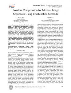
Because of the interference caused by the harsh drilling environment [10], sensors may get singular values sometimes. The singular values are useless for drilling work. Moreover, they often enlarge the value range of the correct data, which increases DPCM error and brings down the performances of data coding. So we use the 3σ criterion [11] to detect singular values and replace them with the average value. 3σ criterion is used widely in electronic measurement to remove abnormal data effectively. Supposing X is the average of X i , σ is
0.031
probability
A. Logging Data Preprocessing To enhance the encoding performance, we have to preprocess logging data with removing singular value and translation transformation at first. Considering the limitation of low power consumption and poor computing capability of the drilling instruments, preprocessing should be simple and have low computational complexity.
We find that all five wells’ EWR data have no value between 64 and 106. The reason is that the geological characteristics determine the logging data’s distributing intervals. Fig. 4 shows the translation transformation of DEEP data. We move the values which are less than 64 to close to 106. Consequently, a narrow value range of logging data is obtained. The receiver recovers the data via the inverse transformation of the values. 0.021 0.010 0
0
100
50
150
200
250
DEEP data value (a) DEEP data original value probability distribution map probability
254~1909 meters and the total drilling time is about 190 hours. Moreover, the amount of the total logging data we use is 461,784 bits.
0.031 0.021 0.010 0
0
50
100
150
200
250
DEEP data value (b) DEEP data translation transformation probability distribution map
the standard deviation. If X i − X > 3σ , then X i is a
Figure 4. Translation transformation
singular value, replace X i with X . To reduce computational complexity, we use formula (3) to get σ.
B. Encoding Experiments We define the encoding distortion as d to evaluate encoding performance. The encoding distortion d is the ratio of the mean square deviation and the mean value of original data, which is formulated by Equation (4).
N ∑ i =1 X i 2 − (∑ i =1 X i ) 2 N
σ=
N
(3) N2 According to formula (3), in order to obtain the standard deviation σ, we only have to do the extraction operation once, do the multiplication operation five times and do the addition operation three times. The computational complexity is constant and does not increase with the growing of data quantity N . So the time complexity is O(1) . DGR value
150 100 50 0
0
1000
2000
3000
4000
5000
DGR sample (a) DGR original curve
N
N
i =1
i =1
d = ∑ ( X i − Yi ) 2 / ∑ X i
(4)
Where X i is the value of the i -th original sample and Yi is the decoded value of the i -th sample. Table II gives the DGR encoding distortion when using different order predictive function and different code length. The results show that the influence of predictive function order is less than that of the code length. Based on the encoding distortions of Table II, we choose 2 or 3 bits to encode DGR data in practical production. In this paper, the criteria of code length selection are d < 5% . Obviously, one order predictive function and 3-bit length are the best choice to encode the 8-bit original DGR data.
DGR value
150
TABLE II DGR LOGGING DATA DISTORTION
100 50 0
Order 0
1000
2000
3000
4000
5000
DGR sample (b) DGRcurve after removing singular value
Figure 3. Removing singular value
Figure3 (a) shows the data curves before removing the singular values, which is the original output of sensor. Figure3 (b) shows the data curves that we had removed singular data from normal data. Comparing Figure3 (a) and (b), we find 3σ criterion is effective to remove abnormal logging data. After removing the singular values, the data value range reduce to 20~56 from 18~141. © 2010 ACADEMY PUBLISHER
DPCM Code Length 2bit
3bit
4bit
5bit
1
0.0733
0.0332
0.0125
0.0040
2
0.0651
0.0202
0.0062
0.0024
Table III shows the encoding performance when using one order predictive function and 3 bits to encode the 8bit original DGR data. The first row of Table III is the well ID of the training data. The first column is the well ID of encoding data. The values of Table III are the values of distortion d . The results show that all the values of d are less than 5%.
284
JOURNAL OF SOFTWARE, VOL. 5, NO. 3, MARCH 2010
TABLE III. DGR ENCODING PERFORMANCE Encoding
TABLE V. DEEP ENCODING PERFORMANCE
Training Set Well ID
ll No. 1
No. 1
No. 2
No. 3
No. 4
No. 5
Encoding Well ID
No. 1
No. 2
No. 3
No. 4
No. 5
0.0300
0.0373
0.0351
0.0273
0.0329
No. 1
0.0470
0.0253
0.0333
0.0323
0.0267
No. 2
0.0317
0.0337
0.0337
0.0288
0.0311
No. 2
0.0726
0.0374
0.0554
0.0487
0.0412
No. 3
0.0305
0.0334
0.0341
0.0286
0.0314
No. 3
0.0848
0.0393
0.0451
0.0448
0.0364
No. 4
0.0248
0.0325
0.0309
0.0239
0.0290
No. 4
0.0903
0.0327
0.0446
0.0444
0.0394
No. 5
0.0255
0.0332
0.0329
0.0279
0.0298
No. 5
0.0368
0.0274
0.0399
0.0323
0.0275
Through analyzing Table III, we find that the maximum of d is 0.0373 and the minimum of d is 0.0239, which means different training set has a little influence on DGR encoding performance. DGR value
60 50 40 30 20
0
200
400
600
800
1000
1200
1400
1600
1800
2000
1600
1800
2000
DGR sample (a) DGR original curve(8bit encode)
DGR value
60 50 40 30 20
0
200
400
600
800
1000
1200
1400
DGR sample (b) DGR decoding curve(3bit DPCM)
Training Set Well ID
Table V shows the encoding performance when using one order predictive function and 4 bits DPCM to encode the DEEP data. The first row of Table V is the well ID of the training data. The first column is the well ID of encoding data. The values of Table V are the values of distortion d .The maximum of d is 0.0903 and the minimum of d is 0.0253. Compare with Table III, we can state that different training data has greater influence on the encoding performance of the DEEP data than on the DGR data encoding performance. Moreover, the smaller the training set is (for example, the amount of data of well 1 is 29184 bits), the worse the encoding performance is (the maximum of d is 0.0903), and the bigger the training set is (for example, the amount of data of well 5 is 86848 bits), the better the encoding performance is (the maximum of d is 0.0412). So we select large training set, such as the well 2 and well 5, to compute the DEEP data encoding parameter in practical production. In this case, d is less than 5%.
TABLE IV. Type DEEP
SHALLOW
Order
250 200 150 100 50
200
400
800
1000
1200
1400
1600
1800
2000
1600
1800
2000
250 200 150 100 0
200
400
600
800
1000
1200
1400
DEEP sample (b)DEEP decoding curve(4bit DPCM)
DPCM Code Length 2bit
3bit
4bit
5bit
1
0.3081
0.0851
0.0274
0.0126
2
0.2714
0.0798
0.0285
0.0120
1
0.3114
0.1079
0.0314
0.0159
2
0.2698
0.0727
0.0243
0.0099
Table IV shows the EWR encoding distortion when using different order predictive function and different code length. We can see that the influence of predictive function order is less than that of the code length as same as DGR data encoding. According to the values of d showed in Table IV, we can select 3 or 4 bits to encode the EWR data, i.e., the DEEP data and the SHALLOW data, in practical production. In this paper, we select the one order predictive function and 4 bits to encode 8-bit original DEEP/SHALLOW data.
© 2010 ACADEMY PUBLISHER
600
(a) DEEP original curve(8bit encode)
50
EWR LOGGING DATA DISTORTION
0
DEEP sample
DEEP value
Fig. 5 compares the original DGR data with the DPCM decoded DGR data under d = 0.0373 , which is the maximum of d in Table III. Something need to be stressed is that d is the maximal can be seen as the worst case. The result shows that the two curves have the same changing trend. That is to say, our method does not disturb LWD user’s qualitative analysis even in the worst case when using one order predictive function and 3 bits DPCM to encode the 8-bit original DGR data.
DEEP value
Figure 5. Original DGR curve and decoding curve when d=0.0373
Figure 6. Original DEEP curve and decoding curve when d=0.0903
Fig. 6 compares the original DEEP data with the DPCM decoded DEEP data under d = 0.0903 , which is the maximum of d in Table V. The result shows that the two curves have the same changing trend. That is to say, our method does not disturb LWD user’s qualitative analysis in the worst case when using one order predictive function and 4 bits DPCM to encode the 8-bit original DEEP data. TABLE VI. SHALLOW ENCODING PERFORMANCE Encoding Well ID
Training Set Well ID No. 1
No. 2
No. 3
No. 4
No. 5
JOURNAL OF SOFTWARE, VOL. 5, NO. 3, MARCH 2010
285
No. 1
0.0206
0.0201
0.0237
0.0214
0.0203
No. 2
0.0254
0.0248
0.0314
0.0295
0.0299
No. 3
0.0291
0.0226
0.0251
0.0273
0.0260
No. 4
0.0536
0.0360
0.0390
0.0328
0.0312
No. 5
0.0226
0.0214
0.0271
0.0258
0.0252
the encoding distortion rates about the four kinds of data when using one order predictive function and different code length. TABLE VII LOGGING DATA DISTORTION DPCM Code Length
Type
3bit
4bit
5bit
0.1600
0.0548
0.0229
0.0100
NEAR
0.1194
0.0591
0.0194
0.0172
FAR
0.1080
0.0457
0.0172
0.0060
TEM
0.0859
0.0196
0.0147
0.0127
DEN value
160 140 120 100 80
200
0
200
400
600
800
1000
1200
1400
1600
1400
1600
DEN sample (a) DEN original curve (8 bit encode)
150 100 0
200
400
600
800
1000
1200
1400
1600
1800
2000
DEN value
160
50
SHALLOW sample (a) SHALLOW original curve(8bit encode)
140 120 100 80
200
0
200
400
600
800
1000
1200
DEN sample (b) DEN decoding curve (3 bit DPCM)
150 100 50
Figure 8. Original DEN curve and decoding curve when d=0.0526 0
200
400
600
800
1000
1200
1400
1600
1800
2000
SHALLOW sample (b) SHALLOW decoding curve(4bit DPCM)
Figure 7. Original SHALLOW curve and decoding curve when d=0.0536
Fig. 7 compares the original SHALLOW data with the DPCM decoded SHALLOW data under d = 0.0536 , which is the maximum of d in Table VI. The result shows that the two curves have the same changing trend. Thus, our method does not disturb LWD user’s qualitative analysis in the worst case when using one order predictive function and 4 bits DPCM to encode original 8-bit SHALLOW data. C. Other Logging Data Encoding Experiments The similar analyzing approach can be applied to other logging data, such as density, neutron and temperature. To show the effectiveness of our methods, the other four kinds of logging data are experimented, which include the neutron logging data called NEAR and FAR, the density logging data called DEN and the temperature logging data called TEM. The four kinds of data above are also represented with 8bits in existing LWD systems, respectively. However, no source compression has been performed on them. In following tests, our method is executed on them. Table VII gives
© 2010 ACADEMY PUBLISHER
Fig. 8 compares the original density data DEN with the DPCM decoded DEN data under d = 0.0526 . The result shows that the two curves have the same changing trend. 90
NEAR value
SHALLOW value
2bit
DEN
Based on the results of Table VII, we can select 3 or 4 bits to encode the original data in practical production. In this paper, we chose one order predictive function and 3 bits to encode the original density, neutron and temperature data. From Table VII, it can be observed that the distortion is not more than 6%.
80 70 60 50 40
0
200
400
600
800
1000
1200
1400
1600
1400
1600
NEAR sample (a) NEAR original curve (8 bit encode) 90
NEAR value
SHALLOW value
Table VI shows the encoding performance when using one order predictive function and 4 bits to encode original 8-bit SHALLOW data. The first row of Table VI is the well ID of the training data. The first column is the well ID of encoding data. The values of Table VI are the values of distortion d .The maximum of d is 0.0536 and the minimum of d is 0.0201. The result shows that different training data has a little effect on the SHALLOW data encoding performance as same as DGR data encoding. Moreover, Table VI shows most values of d are less than 5%. From the results of the Table VI and the Table V, we can see that the encoding performance of SHALLOW data is better than that of the DEEP data. The reason is that the distribution of SHALLOW data is more centralized than that of the DEEP data as shown in Fig. 1(a) and Fig. 1(b).
80 70 60 50 40
0
200
400
600
800
1000
1200
NEAR sample (b) NEAR decoding curve (3 bit DPCM)
Figure 9. Original NEAR curve and decoding curve when d= 0.0330
Fig. 9 compares the original neutron data NEAR with the DPCM decoded NEAR data under d = 0.0330 . The result shows that the two curves have the same changing trend.
JOURNAL OF SOFTWARE, VOL. 5, NO. 3, MARCH 2010
90
D. Summarization Of The Experiments In this section, we use one order predictive function and 3 bits to encode the original gamma, density, neutron and temperature data, one order predictive function and 4bits to encode the original resistivity data. The extensive experiments show that our method can make the results precise enough ( d < 5% ) with the compression ratio of 50%.
FAR value
286
80 70 60 50
0
200
400
600
800
1000
1200
1400
1600
1200
1400
1600
FAR sample (a) FAR original curve (8 bit encode)
FAR value
90 80 70
IV.
60 50
0
200
400
600
800
1000
FAR sample (b) FAR decoding curve (3 bit DPCM)
Figure 10. Original FAR curve and decoding curve when d= 0.0526
Fig. 10 compares the original neutron data FAR with the DPCM decoded FAR data under d = 0.0526 . The result shows that the two curves have the same changing trend. Fig. 9 and Fig. 10 compare the original neutron data with the DPCM decoded ones. From the two figures, we can obtain the following conclusions. Like the SHALLOW and DEEP, NEAR and FAR are two kinds of measured data come from the same sensor. Moreover, the encoding performance of NEAR data is better than that of the FAR data, which is just like that the encoding performance of SHALLOW is better than that of the DEEP data. The reason is the value range of the shallow formation measured data (SHALLOW and NEAR is smaller than that of the deep formation measured data (DEEP and FAR), which results in that the distribution of the shallow formation measured data is more centralized than the distribution of the deep formation measured data. TEM value
100 90 80 70
0
20
40
60
80
100
120
140
160
140
160
TEM sample (a) TEM original curve (8 bit encode)
TEM value
100 90 80 70
0
20
40
60
80
100
120
TEM sample (b) TEM decoding curve (3 bit DPCM)
Figure 11. Original TEM curve and decoding curve when d= 0.0067
Fig. 11 compares the original temperature data TEM with the DPCM decoded TEM data under d = 0.0067 . The results show that the two curves have the very similar changing trend, and the TEM data has the best encoding performance in all seven kinds of logging data. The reason is that the change of temperature is often very mild, which is very suitable for DPCM.
© 2010 ACADEMY PUBLISHER
CONCLUSION
In this paper, we proposed a novel real-time compression approach. In our approach the DPCM, which is a lossy compression method, is used to compress the most common logging data (gamma, resistivity, density, neutron and temperature data). To improve the compressing performances, we analyzed the drilling data and found that the logging data from different instruments has different characteristic. So, we optimize the compression parameters for different logging data respectively in terms of their own characteristic to insure the distortion sufferable. Extensive experiments are done on the basis of a great deal of real drilling data. Our experiments show that the lossy compression method can give enough precise results when compression ratio is 50% ACKNOWLEDGMENT This work is supported by National High Technology Research and Development Program of China “863 program” No. 2007AA090801-04. REFERENCES [1] G. A. Hassan and P. L. Kurkoski, “Zero latency image compression for real time logging while drilling applications,” Proceedings of MTS/IEEE OCEANS, 2005, vol.1, pp. 191-196. [2] X. P. Liu, J. Fang and Y. H. Jin, “Application status and prospect of LWD data transmission technology,” Well logging technology, vol.32, no. 3, 2008, pp. 249-253. [3] C. W. Li, D. J. Mu, A. Z. Li, Q. M. Liao, and J. H. Qu, “Drilling mud signal processing based on wavelet,” Proceedings of the 2007 International Conference on Wavelet Analysis and Pattern Recognition, Beijing, China, 2007, pp. 1545-1549. [4] J. H. Zhao, L. Y. Wang, F. Li, and Y. L. Liu, “An effective approach for the noise removal of mud pulse telemetry system,” The Eighth International Conference on Electronic Measurement and Instruments, ICEMI’2007, vol. 1, pp. 971-974. [5] X. S. Liu, B. Li, and Y. Q. Yue, “Transmission behavior of mud-pressure pulse along well bore,” Journal of Hydrodynamics, vol. 19, no. 2, 2007, pp. 236-240. [6] C. Y. Wang, W. X. Qiao, and W. Q. Zhang, “Using transfer matrix method to study the acoustic property of drill strings,” IEEE International Symposium on Signal Processing and Information Technology, 2006, pp. 415419. [7] W. Zhang, Y. B. Shi, and Z. G. Wang, “Wavelet neural network method for acoustic logging-while-drilling waveform data compression,” Journal of the University of Electronic Science and Technology of China, vol. 37, no. 6, 2008, pp. 900-903, 921. [8] G. Bernasconi, and M. Vassallo, “Efficient data compression for seismic-while-drilling applications,” IEEE
JOURNAL OF SOFTWARE, VOL. 5, NO. 3, MARCH 2010
Transactions on Geoscience and Remote Sensing, vol. 41, no. 3, 2003, pp. 687-696. [9] Z. X. Han, F. Guo, and L. K. Qin, “A lossless data compression method based on the characteristics of logging data,” Journal of Xi'an Shiyou University (Natural Science Edition), vol.21, no.1, 2006, pp. 61-63. [10] C. H. Lu, T. Zhang, and H. D. Li, “Mud pulse measurement while drilling system,” Geological Science and Technology Information, vol. 24 (sup), 2005, pp. 3032. [11] B. Liu and G. P. Dai, “Adaptive wavelet thresholding denoising algorithm based on white noise detection and 3σ rule,” Chinese journal of sensors and actutors, vol.18, no. 3, 2005, pp. 473-476.
Yu Zhang received his B.S. degree in computer science from Beijing Jiaotong University (formerly knows as Northern Jiaotong University), Beijing, China, in June 2004. He is currently working toward the Ph.D. degree at the Institute of Information Science, School of Computer and Information Technology, Beijing Jiaotong University, Beijing, China. His research interests include digital signal processing, multimedia communication & processing and compressed sensing.
prediction, processing, etc.
Sheng-hui Wang received his Ph.D. degree in Digital Signal Processing from Beijing Jiaotong University in 2007. He is now a lecturer at Institute of Information Science, Beijing Jiaotong University. His main research interests include video coding & transmission, network traffic modeling and embedded technology, digital signal
Ke Xiong received his B.S. degree in computer science from Beijing Jiaotong University (formerly knows as Northern Jiaotong University), Beijing, China, in June 2004. He is currently working toward the Ph.D. degree at the Institute of Information Science, School of Computer and Information Technology, Beijing Jiaotong University, Beijing, China. His research interests include signal processing, multimedia communication, network performance analysis, network resource management, and the QoS guarantee in IP networks.
© 2010 ACADEMY PUBLISHER
287
Zheng-ding Qiu recieved B.S. degree in Communication Engineering in 1967, and M.S. degree in Digital Signal Processing in 1981 from Northern Jiaotong University, Beijing respectively. During 1967 to 1978, he was a communication engineer at LiuZhou Railway Bureau. Since 1981, he worked at Institute of Information Science, Northern Jiaotong University, where he became a lecturer in 1983, an associate professor in 1987 and a full professor in 1991. He was an oversea research scholar at Computer Science Department of Pittsburgh University, U.S.A., and joined in the program of parallel processing in signal processing. During 1999 to 2000, he was an visiting research fellow at Electronic Engineering Lab of Kent University, U.K. and engaged in image processing and biometrics processing program. From 1993 to 2001, professor Qiu undertook program “Research and Implement of Multimedia Conferences Terminal and System” which is one of Chinese Hi-tech projects and program “the Research and Implement of Multimedia Service Platform over IP network” which is a sub-project of Chinese National Ninth Five-year key projects. His research field includes digital signal processing, multimedia communication and processing and parallel processing. He is currently a fellow of Chinese Institute of Communications, a senior member of Chinese Institute of Electronics and Railway respectively.
Dong-mei Sun received her Ph.D. degree in Digital Signal Processing from Beijing Jiaotong University in 2003. She is now an associate professor at Institute of Information Science, Beijing Jiaotong University. Her research interests include biometrics technology, image analysis, pattern recognition, information security and signal processing. Currently Mrs. Sun has been doing some projects supported by National Natural Science Foundation of China, Specialized Research Fund for the Doctoral Program of Higher Education and National Science & Technology Pillar Program. Recently she has been cooperating with Imaging Research Center at University of Cincinnati (USA) on several medical image processing and analysis projects. So far she has published over 40 research papers in the domestic and international scientific journals and conferences.