EVS24 Stavanger, Norway, May 13-16, 2009
Driving cycle characterization and generation, for design and control of fuel cell buses Edwin Tazelaar1, Jogchum Bruinsma1, Bram Veenhuizen1,2, Paul van den Bosch2 1
HAN University (
[email protected]), 2Eindhoven University of Technology
Abstract Optimization routines for battery, supercap and fuel cell stack in a fuel cell based propulsion system face two problems: the tendency to cycle beating and the necessity to maintain identical amounts of stored energy in battery and supercap at the start and end of the driving cycle used in the simulation. A method is proposed to reduce these problems. The proposed method characterizes driving cycles and generates alternative cycles with an arbitrary length from an existing cycle, based on the characteristics of the original. The method is demonstrated with an existing driving cycle for buses and validated with measurements from a trolley bus in the region of Arnhem, the Netherlands. Keywords: Driving cycle, Component sizing, Optimization, Energy management system, Fuel cell bus
1
Introduction
A significant number of fuel cell bus prototypes and first series have been built today [1, 2]. Still there seems no consensus on the size of components like the fuel cell stack, battery and/or supercap. Some buses are essentially battery dominant vehicles [2, 3], while others have a fuel cell stack power rating comparable to that of the electric motor [2]. The robust approach sizes the components of the propulsion line on assumed extreme conditions. Although this results in a propulsion line capable to deal with virtual all circumstances, it will not provide the most fuel efficient solution for normal conditions. A definition of these ‘normal conditions’ is most useful, but as Daimler AG convincingly demonstrated, even the same vehicle is operated very differently depending on traffic environment and culture [4]. A driving cycle is a useful definition of the conditions to be expected. From literature,
standardized driving cycles as the ETC cycle, the WHTC test and the JE05 cycle are available [5]. Although such cycles are primarily designed for emission tests, they are helpful in designing fuel efficient hybrid propulsion systems [6, 7]. When sizing components using optimization techniques as DP (Dynamic Programming [9]) or variations on ECMS (Equivalent Consumption Minimization Strategy [8, 9]), the driving cycles chosen strongly influence the resulting component sizes. Although the use of driving cycles as definition for the expected traffic conditions increases the quality of the design, it also introduces some limitations: • Sizing components on one driving cycle tends to cycle beating: the fuel efficiency of the propulsion system is best for the given cycle, but suboptimal for, or not robust against, other conditions. • Energy management system design is based on simulations of the propulsion system including batteries and/or supercaps [8]. To enable comparison between energy management
EVS24 International Battery, Hybrid and Fuel Cell Electric Vehicle Symposium
1
systems, the amount of stored energy at the start and end of a simulation is forced to be equal [9]. As most cycles only cover a period up to 30 minutes [5], this is a restrictive and unrealistic condition. A comparison between simulations with more cycles of different lengths partly covers this problem.
frequency spectra and speed distribution. Therefore the objective is reduced in defining function f(.) such that emulation of driving cycles with frequency spectrum and speed distribution equal to the original cycle is possible.
2.2 Therefore, it would be convenient to optimize a hybrid propulsion system based on a number of cycles with comparable characteristics, but different in length and time sequence. This article proposes a method to characterize driving cycles and to generate alternative driving cycles from an existing predefined or measured cycle, to reduce the limitations mentioned.
Linear approach
Considering the traffic circumstances as random (white) noise and as input of a linear system with the speed of the vehicle as output, makes an ARMA model estimation [10] of this system possible:
v( k ) =
2 2.1
Method Objective
The speed of a vehicle depends on the previous speed of the vehicle and the response of the driver on the traffic circumstances. This can be expressed as:
v(k ) = f ( v k−1 , e k )
(1)
where v(k) represents the current speed and vk-1 represents the speed history of the vehicle: vk-1 = [v(k-1) v(k-2) .. v(k-n)], where n is the number of samples back in time, relevant to the kth sample. The associated sample time is small enough to include the longitudinal vehicle dynamics. The traffic environment is expressed as ek, observed (measured) by the driver and through gas throttle and brake influencing the speed of the vehicle. Function f(.) includes both the vehicle dynamics and the response of the driver. Ideally, f(.) is known and ek is available as time series, enabling a direct estimation of driving cycle v. Unfortunately, the traffic circumstances which resulted in a driving cycle are not available as time series. Therefore a direct time series prediction is not possible. To cover this, traffic circumstances are considered random (white) noise, influencing the speed of the vehicle. Although prediction is not possible, when f(.) is available, it enables emulation of driving cycles. These alternatively generated driving cycles should resemble their original in terms of
C( q ) e( k ) . A (q )
(2)
Polynomials C(q) and A(q) are respectively numerator and denominator of the LTI transfer function between noise input and output. These polynomials also define the function f(.), more explicitly (a0 = 1 and order m ≤ n):
v(k ) = −a 1 v(k − 1) + .. − a n v(k − n ) + + c 0 e(k ) + .. + c m e(k − m)
(3)
With e(k) white random noise, the polynomials A(q) and C(q) directly relate to the frequency spectrum of the output of the ARMA model. This enables an accurate match between the spectrum of the emulated driving cycle and the frequency spectrum of the original driving cycle. Disadvantage of the LTI model with random (white) noise as input is that the relation between the probability distribution of the noise and the probability distribution of the output is poor [11]. It is demonstrated that for stable LTI transfer functions and different probability distributions of the noise, the differences in probability distribution at the output reduce as the time of exposure to the excitations increases and the system reaches the stationary state [12]. For the emulation of driving cycles, an accurately defined speed distribution is important, which makes the ARMA model a less suitable choice. An extension to non-linear filters enables stationary random processes with the same spectral density but with different probability distributions. Differential equations of the Itô type [13] have drift and diffusion coefficients that determine the spectral density and probability density of the filter
EVS24 International Battery, Hybrid and Fuel Cell Electric Vehicle Symposium
2
2.3
Proposed method
The method tries to extend the linear approach with a definition of the speed distributions directly at the output of the filter. Again the traffic circumstances are considered random white noise. As the ARMA model estimations show an order m of the numerator equal to one suffices for the driving cycles examined, it is also assumed that the drivers’ response is dominantly the result of his last observation e(k). Traffic circumstances e(k) is stated to equal random white noise sample ξ uniformly distributed between 0 and 1. With this assumption, characterization f(.) (1) reduces to:
v(k ) = f ( v k −1 , ξ) .
velocities vk-1. The history taken into account and defined by n is based on the amount of correlation between sample v(k) and sample v(k-n). With the definition of the conditional probability density function F, a new driving cycle with characteristics comparable to its original is generated using:
vˆ(k ) = v | F( v, vˆ k −1 ) = ξ .
(7)
Figure 1 illustrates one dimension of the probability density function F, given vˆ k −1 , and how to derive a new speed sample from it.
1 0.9 cumulative probability [-]
output [14]. The use of these non-linear filters for load charachterization is proposed before [15]. Among others, the main disadvantage of these non-linear filters for emulating driving cycles is the inability to exactly match desired boundaries in the probability distribution of the output. For instance, for driving cycles an accurate lower boundary of 0 m/s is important. To realize both accurate frequency spectra and accurate speed distributions, the next method is proposed.
0.8 0.7 0.6 0.5
ξ
0.4 0.3 0.2 0.1 0
(4)
0
2
4
6
8
v
10
12
14
16
18
20
speed [m/s]
^ v
k-1
When the function f(.) is derived from an existing cycle, a new driving cycle is generated as:
vˆ(k ) = f ( vˆ k −1 , ξ) .
for one combination of
(5)
This relation states that the new speed sample in the emulated driving cycle depends on a limited speed history and an independent random variable ξ. The definition of function f(.) determines the resemblance in frequency spectrum and speed distribution between the resulting emulated driving cycle and the original cycle. Based on an existing driving cycle v, probability density function F is defined as:
F( v, v k −1 ) = { p( v(k ) ≤ v | v k −1 } .
Figure 1: Probability density function F(v,
(6)
This probability density function F indicates the probability p the next speed v(k) is equal to or smaller than variable v, given n previous
3
vˆ k −1 )
vˆ k −1 .
Algorithm
The algorithm to derive alternative driving cycles consists of two steps: 1. The construction of the conditional probability density function F from an original driving cycle v (characterization). 2. The simulation of an alternative driving cycle vˆ from the conditional probability density function F (generation). The first step starts with a quantization of the speed samples in the original driving cycle. This quantization is based on a sample time ts and a
EVS24 International Battery, Hybrid and Fuel Cell Electric Vehicle Symposium
3
speed interval ∆v =
v max − v min M
where vmax
and vmin represent the maximum and minimum vehicle speed on the given driving cycle, respectively. The driving cycle is now represented by M discrete speed classes. Every speed falls in a class i, where i ∈ {1,.., M} . Next, a transition summation matrix T is built. This square matrix T ( ∈ ℜ n+1 ) with M rows/columns represents how often a combination of transitions between discrete speeds v(k), v(k-1), .., v(k-n) occurs in the original driving cycle ∀
i (.)∈{1..M }
Ti ( 0 ),..,i ( n ) =
(8)
N
∑ ( v( k ) = v
i ( 0)
∧ v( k − 1) = v i (1) ∧ K ∧ v(k − n ) = v i ( n )
)
k = n +1
with v i ∈ {0, ∆v,K, v max } and N representing the number of observations in the original driving cycle. As example, for the situation with n=1 the transition summation matrix T reduces to the next (2-dimensional) transition matrix (where # stands for the number of transitions in the original driving cycle) # {v ( k − 1) = v 1 ∧ v( k ) = v1 } # {v ( k − 1) = v ∧ v ( k ) = v } 2 1 T ( v) = M # {v( k − 1) = v m ∧ v( k ) = v1 }
{
}
{
}
# v ( k − 1) = v 1 ∧ v ( k ) = v 2
# v ( k − 1) = v 2 ∧ v ( k ) = v 2
L
{
# v ( k − 1) = v M ∧ v ( k ) = v 1
O
{
# v ( k − 1) = v M ∧ v ( k ) = v M
} }
(9) To generate an alternative driving cycle with a length different from its original, the transition summation array T is normalized to the number of samples and multiplied with the desired length of the driving cycle to be generated. Based on the transition summation array of expression (8), given the previous n samples, the probability the next speed sample is less than a certain value is derived as: i (0 )
∑T
j,i (1),..,i ( n )
∀
i (.)∈{1..M }
F( v i ( 0) , v k −1 ) =
j= 0 n
∑T
j,i (1),..,i ( n )
j= 0
. (10)
The second step is the generation of alternative cycles as given by expression (7)
vˆ(k ) = v | F( v, vˆ k −1 ) = ξ .
(7)
As probability density function F is based on the original driving cycle, the distribution of speeds in the alternative cycles will approach asymptotically to the original distribution for long alternative driving cycles. If during generation the original transition summation array T is adjusted according the simulated transition, the distribution of the generated pattern also resembles the original distribution for limited lengths of the alternative driving cycle. In that case, given the generated sample vˆ( k ) = v i ( 0 ) based on the previous transition vˆ( k − 1) = v i (1) , .. , vˆ( k − n ) = v i ( n ) , transition summation array T is updated according:
Ti ( 0),..,i ( n ) = Ti ( 0),..,i ( n ) − 1 .
(11)
Based on this updated transition summation array T, also probability density function F(vi(0),vk-1) is recalculated. As every number in the transition summation array T stands for a transition in velocity, updating according (11) is called ‘pick without return’. Omitting the update (11) is referred to as ‘pick with return’. Advantage of ‘pick without return’ is both a frequency spectrum and a speed distribution of the generated driving cycle equal to the original driving cycle. Disadvantage is the possibility of an unsolvable situation for the next transition simulated, as the remaining combinations T may result in an update of Ti(0),..,i(n) below zero. At that point the algorithm stops. This appears no practical limitation and useful driving cycles are produced still.
4
Results
Method and algorithm are only useful if the generated driving cycles resemble the characteristics of the original driving cycle. This needs a definition of what is a good alternative driving cycle. As it is already concluded that time series prediction of a driving cycle is not possible
with vk-1 = [ vi(1) vi(2) … vi(n) ].
EVS24 International Battery, Hybrid and Fuel Cell Electric Vehicle Symposium
4
due to the random behaviour of the traffic environment, this qualification is based on: • A statistical comparison of original and generated time series, using histograms, • A spectral comparison of original and generated time series, using power spectra. Although also other choices are possible, the comparisons discussed will be limited to the mentioned above. Previous speed versus present speed ( 1 [s]) 20
Speed [m/s]
15
10
5
0
0
5
10 Speed [m/s]
15
20
Previous speed versus present speed ( 3 [s]) 20
Speed [m/s]
15
10
5
0
0
5
10 Speed [m/s]
15
20
Previous speed versus present speed ( 10 [s]) 20
Speed [m/s]
15
10
5
0 0
5
10 Speed [m/s]
15
20
Figure 2: Relation between current velocity and previous velocity (1, 3 and 10 seconds in past).
The method is applied on an existing driving cycle for a bus, the Braunschweig cycle [5]. Figure 2 relates the current speed to the velocity 1, 3 and 10 seconds in the past. From a straight line, this relation shifts to a scatter plot between zero and the maximum velocity. Based on this correlation, the method is applied with a sampling time of 1 second and a history of 3 seconds. The speed is quantized with 17 discrete values for the velocity (M=17). Figure 3 shows the results. The first and second graph show the time series of the original and generated cycle, respectively. A first observation shows that the nature of the generated cycle resembles its original, except for the quantized values for the velocity in the generated cycle. The histogram illustrates that the occurrence of speed values in the original and alternative cycles match closely, although the variant ‘pick with return’ is used. The power spectra of both cycles are comparable, except for high frequency levels, where the sampling in amplitude results in quantization noise above 0,2 Hz in the generated driving cycle. Figure 3 shows the ability of the method to characterize a driving cycle and generated alternatives. To conclude on the practical value of the method, in cooperation with Connexxion/TSN measurements are taken from a bus with an electric propulsion system, a trolley bus in the city of Arnhem, the Netherlands. On the same day a bus route is driven several times in both directions. One of the measured speed profiles is used as input to the proposed method. The resulting speed distributions and power spectra are compared with those of another measured driving cycle. The results are shown in figure 4. Measurements are resampled to a sample time of one second and quantized to 37 speed classes. Again the method correlates the current speed sample with 3 samples in the past and ‘pick with return’ is used, providing the fastest software implementation but possibly deviations in the speed distributions. Again the nature of the original and generated driving cycles resembles. The difference in speed distribution between the original cycle (blue) and the generated cycle (red) lays within the deviation between the two measured cycles along the same route (blue and green). The speed distribution of the generated cycle notably resembles the original cycle more than the alternative measured cycle. Also the spectrum for the generated cycle resembles the spectra of both measured cycles, except for the quantization noise.
EVS24 International Battery, Hybrid and Fuel Cell Electric Vehicle Symposium
5
Original driving cycle Time [s]
20 10 0
0
200
400
600
800
1000
1200
1400
1600
1800
1200
1400
1600
1800
Time [s] Generated driving cycle Time [s]
20 10 0
0
200
400
600
800
1000 Time [s]
Histograms driving cycles
Frequency spectra driving cycles
50
40 30 Speed [m/s dB]
Occurance [%]
40 30 20 10
20 10 0 -10
0
0
2
4
6
8 10 Speed [m/s]
12
14
-20 -3 10
16
-2
-1
10
0
10
10
Frequency [Hz]
Figure 3: Original and generated driving cycle compared on speed distribution and power spectra.
Original driving cycle Time [s]
20 10 0
0
100
200
300
400
500 Time [s]
600
700
800
900
1000
600
700
800
900
1000
Generated driving cycle Time [s]
20 10 0
0
100
200
300
400
500 Time [s]
Frequency spectra driving cycles 40
25
30 Speed [m/s dB]
Occurance [%]
Histograms driving cycles 30
20 15 10 5 0
20 10 0 -10
0
2
4
6
8 10 Speed [m/s]
12
14
16
18
-20 -3 10
-2
-1
10
10
0
10
Frequency [Hz]
Figure 4: Measured (blue) and generated (red) driving cycle compared on speed distribution and power spectra with an additional measured driving cycle (green).
EVS24 International Battery, Hybrid and Fuel Cell Electric Vehicle Symposium
6
5
Discussion
Figure 3 and 4 demonstrate the proposed method is able to characterize a driving cycle and that new alternative cycles can be generated from this characterization. These alternative driving cycles resemble the original in terms of their frequency spectrum and speed distribution. This generation of alternative cycles is useful in optimization routines, to reduce the effect of cycle beating and to overcome the effects of the constraint the stored energy at the start and end of a simulation should equal. These problems are specific to optimization procedures. The observation an emulated driving cycle resembles its original more than two driving cycles measured on the same day along the same route, illustrates the accuracy of the proposed method in terms of frequency spectrum and speed distribution. The method does not extend the information enclosed in the original driving cycle. Already two measured driving cycles on the same day along the same route may differ more in terms of speed distribution than an emulated driving cycle based on the characterization of one measured driving cycle compared to this original cycle. More explicitly, a city bus originally designed on a city cycle as the Manhattan bus cycle [5], will with the aid of the proposed method not transform in a coach able to operate between Stavanger and Oslo. Sizing fuel cell stack, battery and/or supercap directly on the conditional probability density function as characterization of an original driving cycle is subject of further study.
6
Conclusions
Driving cycles are an important specification of what is expected from a fuel cell based power train for a vehicle such as a fuel cell bus. Still component sizing based on one or two driving cycles tends to suboptimal solutions, due to risk of cycle beating and the restrictive constraint that energy stored in the system should be equal at the start and end of a simulation. A characterization of the driving cycle and the
generation of alternative cycles with a considerable longer time span would reduce these problems of suboptimality. Apart from the time series representation, a driving cycle can be represented by its frequency spectrum and probability density function. The proposed method explicitly uses these representations. It creates alternative driving cycles comprising the same information as the original driving cycle in terms of frequency spectrum and speed distribution, but with a user defined length. Using both the original driving cycle and the emulated driving cycles in optimization procedures reduces the risk of cycle beating and limits the effect of the constraint concerning the stored energy on the resulting optimal component sizes.
References [1]
Saxe M., Folkesson A., Alvfors P., Energy system analysis of the fuel cell buses operated in the project: Clean Urban Transport for Europe, Energy, 2008
[2]
Harris K., Comparison of four fuel cell battery hybrid power trains for bus applications, proc. Electric Vehicle Seminar, 2007
[3]
Hill D., Battery dominant fuel cell hybrid electric bus, proc. Electric Vehicle Seminar, 2007
[4]
McGuire T., et.al., Analyzing test data from a worldwide fleet of fuel cell vehicles at Daimler AG, The Mathworks News&Notes, 2008
[5]
Dieselnet, www.dieselnet.com, 2008
[6]
Gökdere L.U., et.al., A virtual prototype for a hybrid electric vehicle, Mechatronics, 2002
[7]
Corbo P., et.al., An experimental study of a PEM fuel cell power train for urban bus application, J. of Power Sources, 2007
[8]
Guzzella L., Sciaretta A., Vehicle propulsion systems; Introduction to modeling and optimization, Springer, 2005
[9]
Rodatz P., et.al., Optimal power management of an experimental fuel cell/supercapacitor-powered hybrid vehicle, Control Engineering Practice, 2005
[10] Ljung L., System identification; Theory for the user, Prentice Hall, 1999 [11] Ludeman L.C., Random Processes: Filtering, Estimation, and Detection, Wiley, 2003
EVS24 International Battery, Hybrid and Fuel Cell Electric Vehicle Symposium
7
[12] Wu C., Cai G.Q., Effects of excitation probability distribution on system responses, Int. J. Non-Linear Mechanics, 2004 [13] Itô K., On stochastic differential equations, American Mathematical Society, 1951 [14] Cai G.Q., Wu C., Modeling of bounded stochastic processes, Probabilistic Engineering Mechanics, 2004 [15] Gamou S., Yokoyama R., Ito K., Optimal unit sizing of cogeneration systems in consideration of uncertainty energy demands as continuous random variables, Energy Conversion and Management, 2002
Authors Edwin Tazelaar received his master’s degree in Electrical Engineering from the Eindhoven University of Technology in 1992. He worked in the fields of control systems, power plants and high power semiconductors for KEMA and Philips Semiconductors. Currently he is researcher on fuel cell based propulsion lines and manager of the Master program Control Systems Engineering, at the HAN University of Applied Science in Arnhem, the Netherlands. Jogchum Bruinsma studied Electrical Engineering and holds a master degree in Control Systems Engineering from the HAN University of Applied Science, Arnhem. As design engineer he contributed in the automation of fuel cell propulsion systems for ships at Alewijnse. Currently he works as automation engineer at Royal Boskalis Westminster.
Paul van den Bosch obtained his master's degree in Electrical Engineering and PhD degree at Delft University of Technology, where he was appointed full professor in Control Engineering in 1988. In 1993 he was appointed to the Measurement and Control Chair in the Department Electrical Engineering at the Eindhoven University of Technology. He authorized over 225 scientific publications and supervised about 40 PhD students. His main research interests deal with modelling and control issues related to industrial processes and automotive applications.
Bram Veenhuizen received his master’s degree and PhD degree on from the University of Amsterdam in 1984 and 1988 respectively. He joint SKF focussing on electromagnetic and X-ray techniques to characterize materials and material fatigue. In 1995 he joined van Doorne’s Transmisie, where he was responsible for the realization of some advanced drive train projects. In 2002 he was appointed assistant professor at the Eindhoven University of Technology. Since 2005 he is also professor in vehicle mechatronics at the HAN University of Applied Science.
EVS24 International Battery, Hybrid and Fuel Cell Electric Vehicle Symposium
8