International Journal of Automotive and Mechanical Engineering ISSN: 2229-8649 (Print); ISSN: 2180-1606 (Online); Volume 14, Issue 3 pp. 4508-4517 September 2017 ©Universiti Malaysia Pahang Publishing DOI: https://doi.org/10.15282/ijame.14.3.2017.9.0356
Characterisation and development of driving cycle for work route in Kuala Terengganu I. N. Anida, I. S. Ismail, J. S. Norbakyah, W. H. Atiq and A. R. Salisa* School of Ocean Engineering, Universiti Malaysia Terengganu, 21030 Kuala Terengganu, Terengganu, Malaysia *Email:
[email protected] ABSTRACT Driving cycle is essential for researchers and also vehicle developers to study the performance of the vehicle mainly via simulations. However, the driving cycles are not the same for different countries or cities, although they may seem identical. In this paper, several driving cycle data were collected for different routes in Kuala Terengganu city at peak hours which were then split into several micro-trips. A genetic algorithm was used as a procedure for selecting the optimised micro-trip to develop a complete Kuala Terengganu driving cycle. Then, the proposed driving cycle was compared with other existing driving cycles such as Urban Dynamometer Driving Schedule, Highway Fuel Economy Test Cycle, Supplemental Federal Test Procedure and Environmental Protection Agency. The proposed complete Kuala Terengganu driving cycle was successfully developed with 10 micro-trips and a total time of 1600s. The results showed that the comparison of percentages error for characteristic parameters for the KT and UDDS driving cycle was the lowest at 161.4 percent compared to others. This indicated that KT driving cycle and UDDS driving cycle is similar to each other as the driving cycle for cities. As a conclusion, the KT driving cycle was successfully obtained using the GA method with all of the percentage error for all parameters of below 10 percent, except for the percentage of cruise time. The results for the comparison also proved that the KT driving cycle is similar to UDDS driving cycle where both are the driving cycle for cities. Keywords: Driving cycle; micro-trip; optimisation; genetic algorithms, UDDS, EPA, HWFET INTRODUCTION Vehicle driving cycle is a series of point for speed of vehicle versus time which is mainly used to evaluate the performance of either the vehicle or engine. Most of the researches on driving cycle are based on the conditions of vehicle in a specific location such as the United States FTP75, Europe ECE15, and Japan 10115. These driving cycles are widely applied for evaluating the performance of the vehicle emission, fuel consumption, traffic condition and also for designing, developing and modelling new vehicles, especially hybrid vehicles [1-3]. The construction of the driving cycle starts with the data collection of the actual driving cycle of the vehicle. Generally, there are two methods on data collection of the driving cycle known as the chase car method and on board measurement method [4]. The chase car method uses the vehicle that can measure the speed data. Then, the vehicle is used to chase the reference or target car in a predetermined route. Meanwhile, the on board measurement method uses a specific device for requiring the 4508
Characterisation and development of driving cycle for work route in Kuala Terengganu
driving cycle data in the vehicle. The speed data is collected by the device when the vehicle travels through the selected route. In recent years, several methods were proposed for the development of the driving cycle such as micro-trip based cycle construction, segment-based cycle construction, pattern classification cycle construction, and modal cycle construction [4]. The construction of the driving cycle based on micro-trip is a combination of short driving cycle to form a complete driving cycle. Usually, these short driving cycles are taken from a collected driving cycle which is between two adjacent stops including idle periods. The combination of the micro-trip cycle to form the driving cycle can be based on two methods; driving cycle parameter and speed-acceleration frequency. As presented in [5-9] the characteristic parameters such as average speed, average driving speed, average acceleration, average deceleration, percentage of idle, cruise, acceleration, and deceleration are used as a guideline for choosing the micro-trip as members in the complete driving cycle. The selection of the micro-trip and complete driving cycle is based on comparison between the target parameters and also new parameters of the driving cycle. Meanwhile, the driving cycle construction based on speed-acceleration frequency is grouping the micro-trips based on their speedacceleration parameters as presented in [10]. The micro-trips in the respective group are than selected to from the driving cycle based target parameter. The major limitation of micro-trip based cycle construction is that it is not possible to differentiate micro-trips by various types of driving conditions such as roadway type or Level of Service (LOS) as explained by [11]. However, since micro-trip based cycle construction covers each ‘stopgo’ condition, it will be a better approach for emission purpose and fuel estimation purpose. In this paper, a new driving cycle was proposed and developed for Kuala Terengganu (KT) city in Malaysia. The route selection for the driving cycle data collection focused on the main route used by drivers to go to and back from work. Several micro-trips from the actual driving cycle data were selected for a complete drive cycle using Genetic Algorithms (GA) for error optimisation. The remainder of this paper is organised as follows. In Section 2, the data analysis is explained which covered the route and time of the driving cycle, micro-trip construction and driving cycle data characterisation. Next, the methodology of the construction of KT driving cycle city is explained in Section 3 including the optimisation using the GA method. The results and discussions including comparison of the driving cycle with existing driving cycles such as UDDS, HWFET, US60, and EPE are discussed in Section 4. Finally, the development of the KT driving cycles is concluded in Section 5. METHODS AND MATERIALS Data Analysis There were three selected routes from the initial location to the final location for the test vehicle to collect the speed-time data. The data were collected at the peak hour where workers went to work (GTW) and also back from work (BFW) which was at 7 am and 5 pm, respectively. The route was selected based on the main route used by most of the drivers going to work from the initial location to the final location. The data were collected for different route at several times. This step was repeated for both GTW and BFW conditions.
4509
Anida et al. / International Journal of Automotive and Mechanical Engineering 14(3) 2017 4080-4096
Micro-trip The development of the KT driving cycle was based on the micro-trips method. In this research, the micro-trip was considered as the short drive cycle with two idle points at the beginning and the end. From a total of 30 drive cycles, N from the data collection, there were 302 micro trips, M. Each of the micro trip was arranged by the assigned number, MTi and the number of which drive cycle it belonged to, DCj where i = 1,2,3…N and j = 1,2,3…M. Figure 1 shows an example of the micro-trip from the actual KT driving cycle. Micro-trip 73 12
5
10
4
8
Speed (m/s)
Speed (m/s)
Micro-trip 33 6
3
6
2
4
1
2
0
0
10
20
30 Time (s)
40
50
60
0
0
20
40
60 Time (s)
80
Figure 1. Example of micro-trip from actual KT driving cycle. Table 1. General parameters for drive cycle characteristics. No. 1 2 3 4 5 6 7 8 9 10 11 12 13 14 15 16 17 18 19 20 21 22 23
Parameters Total Distance Total time Driving time Idle time Cruise time Maximum speed Average speed Average driving speed Standard deviation of speed Maximum acceleration Acceleration time Average acceleration Standard deviation of acceleration Maximum deceleration Deceleration time Average deceleration Standard deviation of deceleration Percentage of time driving Percentage of idle time Percentage of cruise time Percentage of acceleration Percentage of deceleration Root mean square 4510
Unit m s s s s km/h km/h km/h km/h m/s2 m/s2 m/s2 m/s2 m/s2 m/s2 m/s2 m/s2 % % % % % m/s2
100
120
Characterisation and development of driving cycle for work route in Kuala Terengganu
Data Collection Table 1 shows some of the general parameters for drive cycle characterisation. In this research, nine parameters from the list were used as a baseline for micro-trips selection in the development of the driving cycle. The characteristic parameters of the driving cycle are shown in Table 2 which were used to calculate the target parameters. Target parameters were defined as the average values of the parameters for all collected driving cycle data. Table 3 shows some of the calculated target parameters based on equations from Table 2. Table 2. Characteristic parameters of driving cycle. No. 1 2 3 4 5 6 7 8 9
Parameters Abbreviation Unit Average speed Vavg m/s Average driving speed Vavg_drv m/s Average acceleration Accavg m/s2 Average deceleration Dccavg m/s2 Percentage of idle time %idle % Percentage of cruise time %cruise % Percentage of acceleration %Acc % Percentage of deceleration %Dcc % Root mean square RMS m/s2
Table 3. Mean value of parameter for each route. Route (Run) 1 (GTW) 1 (BFW) 2 (GTW) 2 (BFW) 3 (GTW) 3 (BFW) Average value (Target parameter)
Vavg (m/s) 12.2861 6.7080 12.1608 8.6277 12.0903 5.6126
Vavg_drv (m/s) 13.8390 9.5858 13.7584 12.0557 14.0087 9.8827
Accavg (m/s2) 0.3449 0.3791 0.3385 0.3352 0.3636 0.4160
Dccavg (m/s2) -0.3907 -.04087 -0.3753 -0.3846 -0.4241 -0.4597
%idle (%) 10.8043 31.6817 11.2594 28.7568 13.2901 42.9815
9.5809
12.1886
0.3629
-0.4072
23.1290
Table 3. Continued. Route (Run) 1 (GTW) 1 (BFW) 2 (GTW) 2 (BFW) 3 (GTW) 3 (BFW) Average value (Target parameter)
%cruise (%) 0.3600 1.2544 0.5247 1.4608 0.2862 0.3244
%Acc (%) 47.0619 34.9846 46.3793 37.2787 46.4224 29.8390
%Dcc (%) 41.7738 32.0793 41.8366 32.5037 40.0013 26.8390
RMS (m/s2) 0.5096 0.6802 0.5100 0.6438 0.5126 0.7544
Time (s) 1090.4 2132.8 1105.6 1538.0 1044.6 2598.8
0.7017
40.3276
35.8416
0.6018
1585.0
4511
Anida et al. / International Journal of Automotive and Mechanical Engineering 14(3) 2017 4080-4096
From Table 3, the characteristics of the driving cycle for each road were able to be analysed. The total time for data driving cycle, back from work of road 3 showed that the driver spent the longest time to drive from the final location back to the initial location. The idle time for the driving cycle was the longest compared to others which showed that there were more traffics and the vehicle needed to stop frequently. Construction of KT Driving Cycle Genetic algorithms (GA) is one of the evolutionary computing techniques based on both principles of natural selection and natural genetics; the process that drives biological evolution. The algorithm starts with creating a random initial population. Then, a series of new population is created based on the old population called generation. To create a new population, the algorithm applies a selection of individual as parents for the next population based on their fitness value. The next generation is produced by a combination of crossover and mutation of parents from the previous generation. The children from the previous generation became parents for the next generation. Usually, GA is required to find the minimum value of the fitness function. In GA, the term fitness function or objective function is the function that needs to be optimised. The fitness function consists of individual, which is the potential solution to the optimisation problem. A group or array of individuals known as population or in other word the population is the potential solution for optimisation problem. The smallest fitness function value for any individual in the population is the solution for the optimisation problems. The development and construction of the proposed KT driving cycle used the MATLAB platform. As explained earlier, the proposed driving cycle was a combination of several micro-trips from the actual driving data. The total time of the proposed driving cycle was the average value of total time from all collected data. The selection of micro-trips for the proposed driving cycle was used a procedure created in MATLAB. The procedure started with calculating all the characteristic parameters of the collected data and micro-trip data. Then the average values of the mean values of all collected data were calculated and they were known as the target value. The GA was used by selecting a set of micro-trips MTset = {MT1, …, MTk, …, MTK}, 1 ≤ k ≤ K, to form a complete proposed driving cycle. Take note that, the GA used in this study utilised the optimisation toolbox available in MATLAB. The GA parameters were set to be default values. The objective of using GA was to find the optimised set of micro-trips by minimising the fitness function. The fitness function in this study referred to the total percentage error, e between individual errors of the calculated characteristic parameters of the proposed driving cycle with the target parameters. The fitness function, f1 was defined as: 𝑒=
|𝑐𝑎𝑙𝑐𝑢𝑙𝑎𝑡𝑒𝑑𝑙 −𝑡𝑎𝑟𝑔𝑒𝑡𝑙 | 𝑡𝑎𝑟𝑔𝑒𝑡𝑙
× 100%
𝐿𝐿 = 𝑒 − 𝑒 × 10% 𝑈𝐿 = 𝑒 + 𝑒 × 10% 𝐿 𝑓1 = arg min ∑𝐾 𝑘=1 ∑𝑙=1(𝑒),
4512
(1)
𝐿𝐿 ≥ 𝑒 ≥ 𝑈𝐿
(2) (3) (4)
Characterisation and development of driving cycle for work route in Kuala Terengganu
Start Data for driving cycle (Speed VS Time) Compute target parameters
Generate Micro-trip
GA selected the set of microtrip, MTset Calculate target parameters for MTset
Fitness function is minimised?
No
Yes Calculate idle times between micro-trip, Ti Arrange the MTset together with the Ti for complete KT driving cycle End
Figure 2. Flowchart of the construction of the KT driving cycle. where l is the number of characteristic parameters of the driving cycle, k is the number of micro-trips for the complete driving cycle and K is the predetermined number of the micro-trip. The individual percentage error between the calculated characteristic parameters and target parameters was set to not be over the upper limit (UL) and not below than the lower limit (LL) where both were set to 10%. The total time, T for the proposed KT driving cycle was set to be 1600s. This value was taken considering the target value from the data collection was 1585s and also for its simplicity. Meanwhile, the idle times, Ti between the micro-trips were set to be the division of the remainder of the total micro-trip times, TMT as shown in equation 5. The flowchart for the complete development of KT driving cycle is shown in Figure 2. 𝑇𝑖 =
[𝑇−∑𝐾 𝑘=1(𝑇𝑀𝑇𝑘 )] 𝐾
4513
(5)
Anida et al. / International Journal of Automotive and Mechanical Engineering 14(3) 2017 4080-4096
RESULTS AND DISCUSSION Figure 3 shows the results from the simulation for the proposed KT driving cycle. The predetermined number of the micro-trip for the complete KT driving cycle was set to be 10. From the figure, it shows that the speed was quite high, indicating that the path was clear without much congested traffic. The micro-trips for the proposed driving cycle also contained a longer time which meant that the vehicle was not having regular ‘stop-go’ conditions which will save much more fuel consumption and emissions. It was noted that, the position of micro-trip in the complete proposed driving cycle may not be consistent each time the procedure was run. The performance of this driving cycle was analysed for percentage error between the target parameters and characteristic parameters. Then, the comparison between the proposed KT driving cycle and existing driving cycle was done. The existing driving cycles used for the comparison were Urban Dynamometer Driving Schedule (UDDS), Highway Fuel Economy Test Cycle (HWFET), Supplemental Federal Test Procedure (SFTP) (US06), and Environmental Protection Agency (EPA). Proposed KT Driving Cycle 25 Micro-trip = 145
Micro-trip = 50
20
Speed (m/s)
Micro-trip = 63
15
Micro-trip = 90
10 Micro-trip = 113
5
0 0
200
400
600
800 Time (s)
1000
1200
1400
1600
Figure 3. The proposed KT driving cycle. Table 4 shows the results of the calculated characteristic parameters for the existing driving cycles which were calculated from the Autonomie software and the proposed KT procedure. Both of characteristic parameter’s values calculated from Autonomie and proposed KT procedure gave similar results for all of the existing driving cycles. These results proved that the procedure used in this driving cycle development was correct. Meanwhile, Table 5 shows the characteristic parameters for the proposed driving cycle, its target parameters, and also the percentage error between the calculated and target parameter. The percentage error for all parameters was below 10 percent as predetermined, except for the percentage of cruise time which was bigger than 10 percent. The exception was made for the percentage error of the percentage of cruise time because its value and error were too low, making the percentage error bigger. As presented in [12], there are a lot of factors that affect the results of the driving cycle which are drivers’ behaviour, environmental factors and many more. 4514
Characterisation and development of driving cycle for work route in Kuala Terengganu
Table 4. Characteristic parameters using Autonomie and proposed procedure of KT driving cycle. No.
Parameters
1 2 3 4 5 6 7
Max acceleration (m/s2) Mean acceleration (m/s2) Max deceleration (m/s2) Distance (miles) Driving time (s) Max speed (mph) Mean speed (mph)
HWFET AN KT 1.4305 1.4305 0.1942 0.1942 -1.4752 -1.4752 10.2568 10.2568 764 764 59.9000 59.9001 48.5847 48.5848
UDDS AN KT 1.4752 1.4752 0.5046 0.5046 -1.4752 -1.4752 7.4504 7.4504 1369 1369 56.7000 56.7001 24.1417 24.1417
Table 4. Continued No. 1 2 3 4 5 6 7
Parameters 2
Max acceleration (m/s ) Mean acceleration (m/s2) Max deceleration (m/s2) Distance (miles) Driving time (s) Max speed (mph) Mean speed (mph)
US06 AN KT 3.7548 3.7548 0.6700 0.6700 -3.0843 -3.0843 8.0073 8.0073 600 600 80.2928 80.2929 51.8455 51.8456
EPA AN 1.4752 0.3856 -1.4752 17.7071 2135 59.9000 34.0703
KT 1.4752 0.3856 -1.4752 17.7071 2135 59.9001 34.0703
Table 5. Characteristic parameters of KT driving cycle. Parameters Average speed (m/s) Average driving speed (m/s) Average acceleration (m/s2) Average deceleration (m/s2) Percentage of idle time (%) Percentage of cruise time (%) Percentage of acceleration (%) Percentage of deceleration (%) Root mean square (m/s2)
Value 9.3960 12.3530 0.3634 -0.3940 23.3125 0.6250 39.5625 36.5000 0.6020
Target 9.5809 12.1886 0.3629 -0.4072 23.1290 0.7017 40.3276 35.8416 0.6018
% Error 1.9303 1.3490 0.1421 3.2605 0.7934 10.9347 1.8973 1.8369 0.0326
The analysis on the comparison of KT driving cycle with the existing driving cycle is as shown in Table 6. The percentage errors between the KT and other driving cycles are also shown in the table together with the value for each parameter. Overall, the UDDS driving cycle showed that the total percentage errors for all parameters were smaller compared to other driving cycles because UDDS is a driving cycle for the city which is similar to KT driving cycle. Other driving cycles such as HWFET, US06 and EPA represented the highway or roadway conditions as explained in [13]. Thus, the results of the parameters will be much more different compared to a city driving cycle. The percentage error of the percentage of cruise time for all driving cycles was highly different compared to KT driving cycle. This result happened because of the behaviour of the drivers in KT city as well as the environmental driving factors. Different cities will reflect 4515
Anida et al. / International Journal of Automotive and Mechanical Engineering 14(3) 2017 4080-4096
different driving habits and driving environments[14]. Since KT is not a big and busy city, the results differed and produced a certain amount of percentage errors with UDDS in which UDDS represented a big and busy city. Table 6 Comparison of characteristic parameters between KT and existing driving cycles. Parameters T (s)
KT 1600
Vavg (m/s)
9.3960
Vavg_drv (m/s)
12.3530
Accavg (m/s)
0.3634
Dccavg (m/s)
-0.3940
%idle
23.3125
%cruise
0.6250
%Acc
39.5625
%Dcc
36.5000
RMS (m/s2)
0.6020
Total error Total error without %cruise
UDDS e (%) 1369 14.4375 8.7520 6.8540 10.7923 12.6342 0.5046 38.8553 -0.5779 46.6751 17.6642 24.2286 7.9562 1173.0 39.7080 0.3678 34.6715 5.0096 0.6764 12.3588 1334.4
HWFET e (%) 765 52.1875 21.5774 129.6445 21.7193 75.8221 0.1942 46.5603 -0.2217 43.7310 0.5229 97.7570 16.6013 2556.2 44.1830 11.6790 38.6928 6.0077 0.2939 51.1794 3070.8
US06 e (%) 601 62.4375 21.4416 128.1992 23.1770 87.6224 0.6700 84.3698 -0.7283 84.8477 6.6556 71.4505 5.4908 778.5 45.7571 15.6578 42.0965 15.3329 1.0550 75.2492 1403.7
EPA e (%) 2136 33.5000 13.3412 41.9881 15.2308 23.2964 0.3856 6.1090 -0.4406 11.8274 11.5637 50.3970 11.0019 1660.3 41.2921 4.3718 36.1423 0.9800 0.5615 6.7276 1839.5
161.4
514.6
625.2
179.2
CONCLUSIONS The characterisation and development of driving cycle for work route in Kuala Terengganu have successfully been done by using GA as an optimisation method to find the optimum micro-trips for a complete proposed KT driving cycle. The data were collected from a predetermined initial location to the final location by three different routes at peak hours. The KT driving cycle was successfully obtained using the GA method with all percentage errors for all parameters of below 10 percent except for the percentage of cruise time. The results for the comparison also proved that the KT driving cycle is similar to UDDS driving cycle where both are the driving cycles for cities. This study should be explored further to analyse the fuel consumption or fuel economy and emissions.
4516
Characterisation and development of driving cycle for work route in Kuala Terengganu
ACKNOWLEDGEMENTS The authors would like to be obliged to Universiti Malaysia Terengganu and Ministry of Education Malaysia for providing financial assistance under project no. 59435. REFERENCES [1] [2] [3] [4]
[5] [6]
[7]
[8]
[9] [10]
[11]
[12]
[13]
[14]
Shi Q, Zheng Y, Wang R, Li Y. The study of a new method of driving cycles construction. Procedia Engineering. 2011;16:79-87. Schwarzer V, Ghorbani R. Drive cycle generation for design optimization of electric vehicles. IEEE Transactions on Vehicular Technology. 2013;62:89-97. Chan CC. The state of the art of electric, hybrid, and fuel cell vehicles. Proceedings of the IEEE. 2007;95:704-18. Galgamuwa U, Perera L, Bandara S. Developing a general methodology for driving cycle construction: comparison of various established driving cycles in the world to propose a general approach. Journal of Transportation Technologies. 2015;5:191. Cheang KM, Wong PK. Development of a Vehicle Driving Cycle for Macau. 2009. Jiang P, Shi Q, Chen W, Li Y, Li Q. Investigation of a new construction method of vehicle driving cycle. Second International Conference on Intelligent Computation Technology and Automation; 2009. p. 210-4. Seers P, Nachin G, Glaus M. Development of two driving cycles for utility vehicles. Transportation Research Part D: Transport and Environment. 2015;41:377-85. Zhang B, Gao X, Xiong X, Wang X, Yang H. Development of the Driving Cycle for Dalian City. 8th International Conference on Future Generation Communication and Networking; 2014. p. 60-3. Zhang F, Guo F, Huang H. A research on driving cycle for electric cars in beijing. IEEE Conference on Control and Decision Conference; 2016. p. 4450-5. Kamble SH, Mathew TV, Sharma G. Development of real-world driving cycle: Case study of Pune, India. Transportation Research Part D: Transport and Environment. 2009;14:132-40. Dai Z, Niemeier D, Eisinger D. Driving cycles: a new cycle-building method that better represents real-world emissions. Department of Civil and Environmental Engineering, University of California, Davis. 2008. Braun A, Rid W. The influence of driving patterns on energy consumption in electric car driving and the role of regenerative braking. Transportation Research Procedia. 2017;22:174-82. BARLOW TJ, Latham S, McCrae I, Boulter P. A reference book of driving cycles for use in the measurement of road vehicle emissions. TRL Published Project Report. 2009. Arun N, Mahesh S, Ramadurai G, Nagendra SS. Development of driving cycles for passenger cars and motorcycles in Chennai, India. Sustainable Cities and Society. 2017;32:508-12.
4517