PROCEEDINGS OF ECOS 2018 - THE 31ST INTERNATIONAL CONFERENCE ON EFFICIENCY, COST, OPTIMIZATION, SIMULATION AND ENVIRONMENTAL IMPACT OF ENERGY SYSTEMS JUNE 17-22, 2018, GUIMARÃES, PORTUGAL
Experimentation and driving cycle performance of three architectures for waste heat recovery through Rankine cycle and organic Rankine cycle of a passenger car engine. Olivier Dumont(CA)a, Rémi Dickesb, Mouad Dinyc, Vincent Lemortd a
Thermodynamics laboratory, Liège, Belgium,
[email protected] b Thermodynamics laboratory, Liège, Belgium,
[email protected] c PSA GROUPE, La Garenne Colombes, France,
[email protected] d Thermodynamics laboratory, Liège, Belgium,
[email protected]
Abstract: The transportation sector needs to decrease significantly its energy consumption. The Rankine cycle (R) and the organic Rankine cycle (ORC) are two of the most promising technologies to convert waste heat from the internal combustion engine (i.e. from exhaust gas and/or engine cooling system) into mechanical or electrical energy. In this paper, three different system architectures are compared using both experimental and modelling investigations. The first architecture consists in a Rankine cycle (using demineralized water as working fluid) using the exhaust gas waste heat of the engine (R-EG), the second cycle consists in an ORC using the thermal power of the engine cooling system (ORC-CE) and the third consists in an ORC using the exhaust gas waste heat (ORC-EG). The advantages and disadvantages in terms of costs, control, influence of ambient conditions, thermal inertia, weight, additional pumping losses due to the eventual addition of a heat exchanger in the exhaust gas line and part load performance of each architecture is detailed. In terms of fuel saving during a standard driving cycle, this study shows that the ORC-CE is the best architecture (3.5%) followed by the ORCEG (3.2%) and finally the R-EG (2.7%).
Keywords: Rankine cycle, organic Rankine cycle, Passenger car, Waste heat recovery, experimental investigation.
1. Introduction 1.1. Context According to the European directive, cars are responsible for about twelve percent of the total EU emissions of CO2 [1]. Roughly one fourth of the combustion energy is converted into useful work. Generally, the major losses during the combustion are known to be heat losses in the engine coolant and heat losses in the exhaust gas. One solution to reduce the car fuel consumption is to reuse the waste heat released in the exhaust gas and/or in the coolant fluid. Many paper in literature study different architectures for waste heat recovery system based on simulations or experimental results ([2] among others). Most of the papers are related to the long haul trucks due to the stable conditions of the source of waste heat compared to a passenger car [3,4,5]. For the passenger car application, few papers discuss the topic. In 2011, an experimental study [6] demonstrated a 0.5 kW (resp. 0.9 kW) average production on an urban cycle (resp. highway cycle) using the exhaust gas heat source. In 2014, Legros [7] investigated a Rankine power system using the exhaust gas as heat source and a tailor-made scroll expander allowing to decrease up to 6.7 g the emissions of CO2 per km. In 2015 [8], the waste heat from the engine cooling system of a stationary engine was able to increase the 1
engine power up to 12% through an organic Rankine cycle power system. In 2017 [9], a 1 kW ORC helped to increase the efficiency of an internal combustion engine of 9.3% using both the engine cooling system and the exhaust gas. Also, the combination of both heat sources could be used with hybrid cars showing up to 8.2% consumption decrease [10]. Based on this state of the art, some work remains to be performed. The aim of this paper is to: - Compare three different architectures of waste heat recovery for a passenger car. - Evaluate the performance of the components and of the global cycle based on an experimental approach. - Calibrate models that are able to predict the performance outside the calibration range. - Simulate the performance in steady-state and on realistic driving cycles for each architecture. - Compare different architectures and heat sources to identify which is the most promising ones according to different criteria (inertia, part-load performance, maturity, among others). After this short introduction, section 2 presents the different experimental set-ups and the modelling methodology. Following this, the experimental results and the calibration of the models is performed in section 3. These calibrated models are used to simulate the performance of the different architectures on different driving cycles. In section 4, a comparison between the three architectures to recover the waste heat from the passenger car is performed and discussed. Finally, the conclusion summarizes the main results and introduces promising perspectives.
2. Methodology 2.1. Case study The case study is a passenger car with a 157 kW gasoline engine (displacement of 1598 cm3) without exhaust gas recirculation (EGR). The exhaust gas temperature varies between 400°C and 800°C while the engine cooling system temperature can vary between 70°C and 120°C. A manual control allows to regulate finely the accelerator pedal to regulate the shaft speed. This engine is connected to a brake, which is water-cooled. The torque of the brake is also regulated manually. A Coriolis mass flow meter measures the fuel consumption while a lambda probe (i.e. an oxygen sensor) measures the proportion of oxygen in the exhaust gases.
2.2. Experimental set-ups Three standard configurations are considered in these experimental investigations (Fig. 1): - A non-recuperative Rankine cycle (demineralized water) using the waste heat available in the exhaust gases (R-EG). - A recuperative organic Rankine cycle power system (R245fa) using the waste heat available in the cooling water of the engine (ORC-CE). - A recuperative organic Rankine cycle power system (R245fa) using the waste heat available in the exhaust gases (ORC-EG). Usually, the simplest way to condense the working fluid is to use the engine cooling system (R-EG). However this would lead to high condensation pressure for the ORC configurations and so to low efficiencies. An air-cooled condenser is therefore preferred for the ORC-EG and ORC-CE configurations. Three test-rigs are designed and built. Their technical specification is detailed in Table 1. R-EG: The sizing of the components of the test-rig has been presented in [7]. In this Rankine cycle, two different evaporator have been tested: a counter current (CC) heat exchanger and a hybrid current (HC) heat exchanger. In a first time, a scroll expander, designed for this application [7] is tested. An axial turbine, designed for μCHP has also been investigated [11]. This turbine requires additional components (a steam trap and an inverted bucket separator to 2
avoid droplets, a second condenser and a void pump to reach the nominal exhaust pressure (≈0.1 bar).
Fig. 1. Schematic representation of the three architectures.
ORC-CE: A 3kWe ORC using R245fa as working fluid is equipped with a recuperator, a brazed plate heat evaporator, an air-cooled condenser and a diaphragm pump. Four types of expanders are tested (Table 1). For more details, please refer to a previous paper [12]. ORC-EG: The same test-rig as for the ORC-CE is used (only the evaporator differs – see Table 1). For more information about the sensors and the detailed layout of each test-rig, please refer to the appendices (Table A1 and Table A2 and Fig. A1-A3) [14].
2.3. Modelling All the components are simulated with semi-empirical models. This kind of models relies on a limited number of meaningful equations that describe the most significant phenomena occurring in the process. Such a modelling approach offers a good compromise between calibration efforts, simulation speed, modelling accuracy and extrapolation capabilities [12,13,15]. The different models parameters are tuned to reach a good match between the measurements and the model predictions. Regarding the heat exchangers, a three-zone moving-boundary model with variable heat transfer coefficients is used. The modelling is decomposed into the different zones of the heat exchanger. Each zone is characterized by a global heat transfer coefficient Ui and a heat transfer surface area Ai. The effective heat transfer occurring in the heat exchanger is calculated such as the total surface area occupied by the different zones corresponds to the geometrical surface area of the component. For more details, see [12]. Volumetric machines are simulated using the grey-box model proposed by [16]. By accounting for the most influent physical phenomena in the expansion process with a limited number of parameters, this model demonstrates a good ability to extrapolate the expander performance out of the calibration 3
dataset while maintaining low computational times. Also, its general formalism allows to model all types of expanders (screw, piston, scroll and root). More details are available in [16].
Component Working fluid
Evaporator
Expander
Pump
Condenser
Table 1. Technical specifications of the test-rigs. Characteristics R-EG ORC-CE Rankine Water R245fa Plate heat Type HC CC exchanger Mass [kg] 3.7 6.54 52 3 Volume [m ] 2.37 1.96 0.009 2 Exchange area (wf) [m ] 0.708 0.254 9.8 Type
Scroll
Turbine Scroll
Volume ratio [-] Swept volume [cm3] Maximal temperature [°C] Maximal pressure [bar] Nominal power [kW] Maximal shaft speed [RPM] Type Swept volume [cm3] Maximal mass flow rate [g/s] Maximal pressure [bar] Type Number Mass [kg] Volume [m3] Water exchange area [m2]
3 8 250 220 20 10 ~4 1.5 15 000 30 000 Gear 0.5 20 (5000 RPM) 20 Brazed plate 1 2 1.05 2.2 1.088 2.05 0.628 0.88
ORC-EG Confidential Confidential Confidential Confidential Screw, piston and root
2.19 12.74 130 See [13] ~1 [1000:8000] [500:5000] Diaphragm 6.8e-6 130 40 Air-cooled 3 14 4.66
The turbine is modeled following a grey box approach, three conservation equations are used to model the turbine (mass flow rate, momentum and total enthalpy) [11]. The windage, mixing and expansion losses are modeled following a former work [17]. The first calibration parameter is used to model the losses in the divergent (entropic loss coefficient) while the second one is used to model the leakage flow [11]. A semi-empirical model is proposed to predict the mass flow rate and the electrical power consumed by the pump (1,2). Equation (1) evaluates the mass flow rate based on the theoretical mass flow rate minus a leakage loss (A) while (2) predicts the power consumption with a constant loss (B), a speed proportional loss (C) and a term proportional to the internal power (D). 𝑚̇𝑤𝑓,𝑝𝑟𝑒𝑑 = 𝜌. 𝑁. 𝑉𝑠 − 𝐴√2𝜌(𝑃𝑒𝑥 − 𝑃𝑠𝑢 ) 𝑊̇𝑒𝑙,𝑝𝑟𝑒𝑑 = 𝐵 + 𝐶. 𝑁 + (1 + 𝐷).
(1)
𝑚̇𝑤𝑓,𝑝𝑟𝑒𝑑 (𝑃𝑒𝑥 −𝑃𝑠𝑢 )
(2)
𝜌
4
Global model Once the models for the different components are calibrated, they are connected together in a way to simulate the complete cycle (Fig. 2). Practically, the model is able to simulate the performance the entire system and can be decomposed in: Inputs: cold sink supply temperature and glide, hot source temperature and flow. Parameters: calibration and geometrical parameters of the pump, evaporator, condenser and expander Control variables: the pump speed is adjusted to get the desired superheating and the expander speed is fixed in a way to optimize the net power. Outputs: working fluid mass flow rate, thermal power in condenser and evaporator, expander power production, pump consumption…
Fig. 2. Modelling of the cycle
2.4. Driving cycle The most common way to evaluate the consumption and the pollution emissions of vehicles is by means of a driving cycle. The New European Driving Cycle (NEDC) (or Motor Vehicle Emissions Group - MVEG), based on a theoretical driving profile, is used in Europe since 1973. From 2017, the Worldwide harmonized Light vehicle Test Procedure (WLTP) should be preferred since the cycle was developed using real-driving data. In this work, both cycles (NEDC and WLTP) are considered. A comparison between the NEDC and the WLTP is given in Table 2. As illustrated, the average values of the speed, mechanical power, exhaust gas thermal power, engine cooling thermal power and exhaust gases temperature are significantly lower for the NEDC. The exhaust gas and engine cooling energy are also presented for two situations: (1) when the inertia of the engine is totally neglected (2) in a more realistic cold start situation (heat not available during 800 s for the engine cooling system and 60 s for the exhaust gases). These time constants come from internal confidential data. The ratios of available thermal energy in the exhaust gas over the engine cooling system are equal to 44% and 64% for the NEDC and WLTP respectively. Therefore the NEDC seems more favorable to the CE architecture than the WLTP. Also, the cold start is unfavorable to the engine cooling system because of its high inertia (Table 2).
5
Table 2. Comparison of the NEDC and WLTP (steady-state, no cold start) Mean values Speed [km/h] Mechanical energy [kWh] Exhaust gas thermal energy [kWh] Exhaust gas thermal energy (cold start) [kWh] Engine cooling thermal energy [kWh] Engine cooling thermal energy (cold start) [kWh] Mean gas temperature [°C]
NEDC 33.8 2.75 1.30 0.91 3.13 1.41 428
WLTP 60.8 7.76 5.02 4.32 6.55 4.40 563
The global improvement of the performance of the engine is evaluated using Equation (3) where 𝑊̇𝑊𝐻𝑅𝑆 is the additional power generated by the considered Waste Heat Recovery System (WHRS), 𝑊̇𝑤𝑒𝑖𝑔ℎ𝑡 is the additional power consumed by the engine because of the additional weight of the WHRS [18] and 𝑊̇𝑃𝑙𝑜𝑠𝑠 is the additional power due to the pumping losses produced in the case of an addition of a heat exchanger in the exhaust gases [19]. In this work, no dynamic is considered. Also, a maximum improvement of performance is evaluated assuming that all the energy produced by the WHRS is useful. ̇
̇
̇
𝑊𝑊𝐻𝑅𝑆 −𝑊𝑤𝑒𝑖𝑔ℎ𝑡 −𝑊𝑃𝑙𝑜𝑠𝑠 𝛥𝑊̇𝑊𝐻𝑅𝑆 = 𝑊̇ 𝑚𝑒𝑐
(3)
3. Results 3.1. Experimental results A global methodology including a cross-checking of the measurements, a Gaussian process to delete measurement outliers and a reconciliation method to improve the quality of the data [20] is applied for each experimental campaign. The performance of each component is evaluated in a wide range of conditions. Here is a summary of the main observations: R-EG: The prototype of pump presents a rather constant volumetric efficiency and an isentropic efficiency (4) reaching 45% (Appendices – Fig. A4), both evaporators presents good performance with efficiencies (6) above 80% (Appendices – Fig. A5) and low pressure drops (Appendices – Fig. A6). However the maximum isentropic efficiencies (5) of the scroll expander (Appendices – Fig. A7) and the turbine (Appendices – Fig. A8) only reach 29% and 42% respectively. The low efficiency of the scroll is explained by high leakages (>50% of the mass flow rate). The turbine cannot be efficient on a real car application since the condensing pressure is very far from the nominal one (0.05 bar). The maximum net production of the cycle is 885 W. ORC-CE: The performance of the four expanders was compared in [13] and are shown in appendices – Fig. A9. To summarize, the scroll expander shows the highest isentropic efficiency (76%), the screw presents a good adaptability to the working conditions over a wide range of shaft speed ([0-20,000] RPM), the piston expander is well suited for high supply pressure and temperature (up to 250°C and 40 bars) and the root expander is working optimally at low pressure ratios (close to one). In the next part of the work, only the scroll is considered because of its higher efficiency. Working with a more adapted volume ratio (close to 3) and an enlarged port diameter could significantly increase the performance. The evaporator presents a pinch point lower than 5K (Appendices – Fig. A10). The pump reaches 6
a maximal efficiency (4) of 31% (Appendices – Fig. A11). The maximum net production of the cycle is 754 W. This value could be increased with an optimal sizing (larger piping to decrease pressure drops and optimal design of the expander). ORC-EG: In the ORC-EG configuration, only the evaporator differs from the ORC-CE layout. This components is rather performing well with an efficiency (6) comprised between 80% and 90% and with pretty low pressure drops on the secondary fluid side (