Drizzle in Stratiform Boundary Layer Clouds. Part II: Microphysical ...

3034

JOURNAL OF THE ATMOSPHERIC SCIENCES

VOLUME 62

Drizzle in Stratiform Boundary Layer Clouds. Part II: Microphysical Aspects R. WOOD Met Office, Exeter, Devon, United Kingdom (Manuscript received 2 April 2004, in final form 16 February 2005) ABSTRACT This is the second of two observational papers examining drizzle in stratiform boundary layer clouds. Part I details the vertical and horizontal structure of cloud and drizzle parameters, including some bulk microphysical variables. In this paper, the focus is on the in situ size-resolved microphysical measurements, particularly of drizzle drops (r ⬎ 20 ␮m). Layer-averaged size distributions of drizzle drops within cloud are shown to be well represented using either a truncated exponential or a truncated lognormal size distribution. The size-resolved microphysical measurements are used to estimate autoconversion and accretion rates by integration of the stochastic collection equation (SCE). These rates are compared with a number of commonly used bulk parameterizations of warm rain formation. While parameterized accretion rates agree well with those derived from the SCE initialized with observed spectra, the autoconversion rates seriously disagree in some cases. These disagreements need to be addressed in order to bolster confidence in large-scale numerical model predictions of the aerosol second indirect effect. Cloud droplet coalescence removal rates and mass and number fall rate relationships used in the bulk microphysical schemes are also compared, revealing some potentially important discrepancies. The relative roles of autoconversion and accretion are estimated by examination of composite profiles from the 12 flights. Autoconversion, although necessary for the production of drizzle drops, is much less important than accretion throughout the lower 80% of the cloud layer in terms of the production of drizzle liquid water. The SCE calculations indicate that the autoconversion rate depends strongly upon the cloud droplet concentration Nd such that a doubling of Nd would lead to a reduction in autoconversion rate of between 2 and 4. Radar reflectivity–precipitation rate (Z–R) relationships suitable for radar use are derived and are shown to be significantly biased in some cases by the undersampling of large (r ⬎ 200 ␮m) drops with the 2D-C probe. A correction based upon the extrapolation to larger sizes using the exponential size distribution changes the Z–R relationship, leading to the conclusion that consideration should be given to sampling issues when examining higher moments of the drop size distribution in drizzling stratiform boundary layer clouds.

1. Introduction In Part I of this study (Wood 2005, hereafter Part I), 12 cases of drizzling stratiform boundary layer clouds are examined, with focus on the horizontal and vertical structure of cloud and drizzle. We extend the study in Part II, with a focus upon size-resolved microphysical observations, particularly of drizzle drops (drop radius r ⬎ 20 ␮m). Microphysical processes are at the heart of many of the current problems associated with aerosol– cloud–climate interactions (Hobbs 1993; Beard and Ochs 1993) and there is a need to better understand the

Corresponding author address: Dr. Robert Wood, Dept. of Atmospheric Sciences, University of Washington, Box 351640, Seattle, WA 98102. E-mail: [email protected]

JAS3530

production and feedbacks of drizzle in marine boundary layer (MBL) clouds. The precipitation rate in drizzling stratocumulus is clearly influenced by cloud droplet concentration (Hudson and Yum 2001; Bretherton et al. 2004; vanZanten et al. 2005; Comstock et al. 2004; and see Fig. 1 in Part I), and it is therefore imperative that accurate parameterizations of the drizzle process are incorporated into climate models if these models are expected to give realistic assessments of the second indirect aerosol effect (Rotstayn and Liu 2005) and cloud–drizzle feedbacks under climate change scenarios. Most warm rain parameterizations are based on the general paradigm, first introduced by Kessler (1969), of treating the condensed water in the cloud as belonging to one of two populations: cloud droplets and raindrops. The former are assumed to be small enough that they do not fall under gravity, whereas the latter have

SEPTEMBER 2005

WOOD

an appreciable terminal velocity. A separation drop radius r0 is chosen to distinguish the two populations. Rate equations are used to express the transfer of water between the cloud and raindrop populations. We can write the water mass transfer rate across the separation radius due to coalescence (COAL) as the sum of two terms: autoconversion (AUTO) and accretion (ACC):

冉冊 ⭸qD ⭸t

⫽ COAL

冉冊 ⭸qD ⭸t

⫹ AUTO

冉冊 ⭸qD ⭸t

.

共1兲

ACC

Autoconversion is defined as the rate of mass transfer from the cloud to the rain population due to the coalescence of cloud droplets (r ⬍ r0). Accretion is defined as the rate of mass transfer from the cloud to the rain population by the coalescence of raindrops (r ⬎ r0) with cloud droplets. Autoconversion depends only upon characteristics of the cloud droplet population, while accretion depends upon both the cloud and the raindrop populations. Expressions for the autoconversion and accretion rates as a function of n(x), the drop size distribution (DSD), where n(x) is the number concentration of drops with mass between x and x ⫹ dx follow from the stochastic collection equation (SCE) with collection kernel K (x, x ⬘) (Beheng and Doms 1986). Autoconversion is expressed as

冉冊 ⭸qD ⭸t

⫽

AUTO

冕再冕 x0

x0

0

x0⫺x

冎

K共x, x⬘兲x⬘n共x⬘兲 dx⬘ n共x兲 dx. 共2兲

Similarly, accretion can be written as

冉冊 ⭸qD ⭸t

⫽ ACC

冕再冕 ⬁

x0

x0

0

K共x, x ⬘兲x ⬘n共x ⬘兲 dx ⬘

冎

n共x兲 dx. 共3兲

Note that the only difference between (2) and (3) is the integral limits. Because of its inherent simplicity, the Kessler paradigm has been widely adopted for the parameterization of rain in all the model frameworks described above (e.g., Tripoli and Cotton 1980; Baker 1993; Beheng 1994; Rotstayn 1997; Wilson and Ballard 1999; Khairoutdinov and Kogan 2000; Liu and Daum 2004). Although other methods exist to parameterize rain, they are generally considerably more computationally expensive (e.g., Tzivion et al. 1987) because they use explicit representations of the DSD and solve the stochastic collection equation. Parameterizations of the Kessler type provide simple expressions for the autoconversion and accretion rates as functions of bulk parameters of the cloud and rain DSD. For each parameterization, these expressions are obtained using one of two basic methods: (i) use a

3035

physical model or make reasonable assumptions to generate a range of DSDs, integrate the SCE for a wide range of DSD parameters, and then provide simple fits such as power laws that relate autoconversion and accretion to bulk parameters (e.g., Kessler 1969; Beheng 1994; Khairoutdinov and Kogan 2000) or (ii) assume a functional DSD form, and then make simplifications to analytical forms for K (x, x ⬘), to arrive at expressions that relate autoconversion and accretion to bulk parameters (e.g., Tripoli and Cotton 1980; Baker 1993; Liu and Daum 2004). Liu and Daum (2004) gives an excellent overview of the assumptions made in parameterizations of autoconversion that use method (ii). The rate terms for the different autoconversion parameterizations vary widely in their dependence upon cloud droplet concentration and liquid water (see Table 1). This is not entirely surprising given the wide range of assumptions that are made in their formulation. Assumptions made about the form of the DSD in one type of cloud may not be appropriate in another. In addition, some of the analytical approximations of the collection kernel are a very poor representation of the true kernel (see, e.g., Liu and Daum 2004). Figure 1 demonstrates graphically just how variable the resulting autoconversion rates are as a function of cloud liquid water content and droplet concentration. For typical droplet concentrations and liquid water contents in MBL clouds, the autoconversion rates from different parameterization vary over three orders of magnitude. In general, the forms for accretion rate are much less variable than for autoconversion (Table 1). What we should conclude from this comparison is that there is a need to constrain the parameterizations in different cloud systems and ask which of them can be used to represent the autoconversion and accretion processes most accurately. In this study aircraft size-resolved microphysical measurements are used as a means to examine microphysical parameterizations in stratiform boundary layer clouds. Microphysical properties of drizzle are of particular importance for the remote sensing problem, especially with the increasing use of ground-based cloud and rain radars in the study of marine boundary layer cloud (Frisch et al. 1995; Yuter et al. 2000; Comstock et al. 2004). In addition, programs are already underway that will mount sensitive millimeter cloud/drizzle radars on spaceborne platforms [e.g., the Cloudsat mission, Stephens et al. (2002), and the planned European Earth Clouds Aerosols and Radiation Explorer (EarthCARE) program]. There is therefore a need to establish retrieval methods for drizzle so that quantitative large-scale observations can begin. Technical limitations will not permit these pioneering spaceborne platforms to make spectral radar measurements such as

3036


VOLUME 62

TABLE 1. Autoconversion and accretion formulations for the four parameterizations examined. Units are kg m⫺3 for liquid water contents, m⫺3 for droplet concentrations, and all droplet radius parameters are in ␮m. The air density ␳ is expressed in units of kg m⫺3. Liquid water density is ␳w, and H(x) is the Heaviside step function.

Scheme Khairoutdinov and Kogan (2000)

Accretion rate (kg m⫺3 s⫺1)

Autoconversion rate (kg m⫺3 s⫺1) ⫺1.79 ⫺1.47 ␳ (A ⫽ 7.42 ⫻ 1013) Aq2.47 L Nd

67 (qLqD)1.15␳⫺1.3 ⫺4

Kessler (1969)

B max(qL ⫺ qL,0, 0) (B ⫽ 1.0d ⫺ 3; qL,0 ⫽ 5 ⫻ 10 )

1/8 0.29qLq7/8 D Nd

Beheng (1994)

⫺3.3 Cd⫺1.7q4.7 (C ⫽ 3.0 ⫻ 1034; d ⫽ 9.9 for Nd ⬍ 200 cm⫺3 L Nd d ⫽ 3.9 for Nd ⬎ 200 cm⫺3)

6.0qLqD

Tripoli and Cotton (1980)

⫺1/3 Dq7/3 H(qL ⫺ qL,0) (D ⫽ 3268, assumes EC ⫽ 0.55 L Nd 4 3 qL,0 ⫽ ␲␳wNdrcm with rcm ⫽ 7 ␮m兲 3

4.7qLqD

Liu and Daum (2004)

10 6 Eq3LN⫺1 d H(R6 ⫺ R6C) {E ⫽ 1.08 ⫻ 10 ␤6, where R6 ⫽ ␤6r␷, 6 2 ␤6 ⫽ [(r␷ ⫹ 3)/r␷] (see text), r␷ is mean volume radius}, 1/2 R6C ⫽ 7.5/(q1/6 L R6 )

N/A

Liu and Daum (2004) (modified)

As above but E ⫽ 1.3 ⫻ 109␤66

N/A

those employed in the state-of-the-art ground-based radar (Frisch et al. 1995), so retrieval of precipitation rate will rely upon reflectivity alone. Thus, there is a need to determine reflectivity–rain rate (Z–R) relationships in drizzling boundary layer cloud. In this study, aircraft data are used to examine the links between radar reflectivity (approximately here by the sixth moment of the DSD) and precipitation rate. This study consists of five sections. In section 2, we describe the measurements of the drizzle drop size distribution (DDSD) and examine the most suitable mathematical form for the description of the DDSD. In section 3, we focus upon drizzle parameterizations. Section 4 examines the relative roles of autoconversion and accretion. Section 5 examines Z–R relationships. The study concludes with a brief discussion of the findings.

2. Drizzle drop size distribution The instruments used to sample the cloud and drizzle size distributions n(r) were described in Part I. Measurements are made using a Particle Measuring System (PMS) Forward Scattering Spectrometer Probe (FSSP) (Baumgardner et al. 1993) and PMS 2D-C optical array probe. The drop radius measurement range spans 1–400 ␮m. Combined FSSP and 2D-C size distributions are produced by linear interpolation in logn(r)–logr coordinates. Here, we take a more focused look at some of the sampling issues and the form that the drizzle drop size distribution (DDSD) takes in stratiform boundary layer clouds. Drizzle drops are defined as those with r ⬎ 20 ␮m. In this section, we examine the mathematical form

FIG. 1. Comparison of parameterized autoconversion rates from widely used schemes [all except the Berry and Reinhardt scheme (Berry and Reinhardt 1974), which is not examined further in this paper, are defined in Table 1]. (a) Autoconversion rate as a function of liquid water content for a fixed cloud droplet concentration of Nd ⫽ 100 cm⫺3. (b) Autoconversion rates as a function of droplet concentration for a fixed liquid water content of qL ⫽ 0.5 g m⫺3.

SEPTEMBER 2005

3037

WOOD

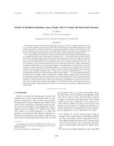
FIG. 2. (a) Normalized DDSDs (R /N )n(r) at all in-cloud levels (103 spectra) plotted against r/R . The universal exponential distribution nexp(r) ⫽ (R /N )n(r) ⫽ exp(⫺r/R ) is shown by the dashed line. The spectra are shown by contours that denote percentiles of all the distributions in each r/R class. The lightest colored contour therefore contains 95% of all the DDSD in each class. (b) As in (a) but normalized DDSDs [rn(r) ln␴/Nln] plotted against ln(r/rG)/ln␴. The universal lognormal distribution nln(r) ⫽ rn(r) ln␴/Nln ⫽ (1/公2␲) exp关⫺ln2(r/rG)2 ln2␴] is shown by the dashed line. See text for the definition of the parameters.

of the DDSD and ask how well we are able to determine the moments of the DDSD, particularly the higher moments that are necessary in making estimations of the precipitation rate and radar reflectivity. The ith complete moment Mi of a DSD n(r) is defined as Mi ⫽

冕

radius rD. We test how well an exponential DDSD represents these data by first normalizing r and n(r). Because our DDSD is necessarily truncated (by design) at r ⫽ r0 ⫽ 20 ␮m, the truncated exponential form is nexp共r兲 ⫽

⬁

r in共r兲 dr

共4兲

r⫽0

with radar reflectivity here approximated by Z ⫽ 26M6, and liquid water content qL ⫽ (4␲ ␳w/3) M3, where ␳w is the density of liquid water. Partial moments, that is, the integral in (4) over a limited radius range, are used to determine cloud (1 ⬍ r ⬍ 20 ␮m) and drizzle (20 ⬍ r ⬍ 400 ␮m) physical parameters. We take DDSDs from the same horizontal layer averages as discussed in Part I. As will be seen, long averaging times are required to sample the larger drizzle drops that can often contribute strongly to the rain rate, and particularly the radar reflectivity. We analyze DDSD results (20 ⬍ r ⬍ 400 ␮m) from all cloud levels, height z with 0 ⬍ z ⬍ 1, where z ⫽ (z ⫺ zCB)/(zi ⫺ * * zCB), and with zCB and zi being the cloud-base and -top heights, respectively. For each measured DDSD, we estimate the drizzle drop concentration Nd,D and mean

冋冉

Nd,D r ⫺ r0 exp ⫺ rD ⫺ r0 rD ⫺ r0

冊册

共5兲

,

where rD is the mean radius of the r ⬎ 20 ␮m drizzle drops. Setting N ⫽ Nd,D exp[r0 /(rD ⫺ r0)] and R ⫽ rD ⫺ r0, we plot the normalized DDSD in Fig. 2a from the entire 12-cloud dataset (103 DDSDs). The collapsed exponential curve nexp(r) ⫽ N /R exp(⫺r/R ) provides a good fit to the normalized spectra, indicating that the truncated exponential form is a good mathematical descriptor of the DDSD. As a comparison, we also attempt normalization using a truncated lognormal distribution given by nln共r兲 ⫽

Nln

公2␲r ln␴

冋冉

exp ⫺

ln2共rⲐrG兲 2 ln2␴

冊册

,

共6兲

where the lornormal parameters are the total drop concentration Nln ⫽ 兰⬁0 nln(r) dr, the geometric mean radius rG, where lnrG ⫽ lnr, and the geometric standard deviation ln␴, where ln2␴ ⫽ ( lnr ⫺ lnrG)2. VanZanten et

3038


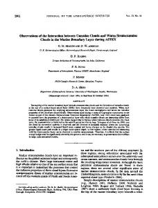
al. (2005) found that the lognormal usefully describes DDSDs in Californian stratocumulus clouds. For each observed DDSD, we estimate the three lognormal parameters and account for truncation at r0 using the method described in Feingold and Levin (1986). The normalization is successful at collapsing the DDSDs onto a universal lognormal function (Fig. 2b). Comparison of the exponential and lognormal forms shows that the lognormal is arguably marginally better than the exponential at describing DDSDs in drizzling stratocumulus clouds. However, the truncated exponential distribution provides almost as good a normalization while requiring only two parameters, and the method to deduce these parameters is very robust (the lognormal fits for truncated distributions were found to be prone to instability). We therefore proceed with the exponential fit for the remainder of this study. Because the exponential provides a good representation of the data, we use the exponential form to assess sampling problems of large drops that stem from the limited sample volume of the 2D-C probe (⬃5 L s⫺1). Because of this and the steep falloff of the exponential distribution, very few drops with radii larger than 200 ␮m were measured on any of the flights, but filter paper measurements show that drops of this size can be present in drizzle (Comstock et al. 2004). We therefore extrapolate the exponential out to sizes larger than those measured and calculate the contribution to Z and precipitation rate R from droplets 60 ␮m ⬍ r ⬍ ⬁, and compare with the contribution only over the measured range. To find the best fit exponential, we use nonlinear least squares fitting over the well-sampled drop range 20 ⬍ r ⬍ 60 ␮m, weighting each size bin using the inverse square of the Poissonian counting error. Rain rate R is estimated using a single drop terminal velocity wT relationship calculated from a fourth-order polynomial fit1 to log10wT, log10r calculated at T ⫽ 280 K and p ⫽ 900 hPa using the full Reynolds number approach described in Pruppacher and Klett (1997). Tests show that the terminal velocities calculated using the single fitted curve differ by no more than 5% from those calculated using the full theory at all temperatures and pressures experienced in this study. Figure 3 shows two examples of the procedure. The DDSDs are shown in the upper panels for two cases. The second row shows the size-resolved reflectivity spectra dZ/dr (filled circles) and precipitation rate spectra dR/dr (diamonds). The exponential fits are shown with dotted (dZ/dr) and dashed (dR/dr) lines, extrapo-

1 log 10 w T ⫽ ⫺3.775 ⫹ 1.468log 10 r ⫹ 0.733(log 10 r) 2 ⫺ 0.366(log10r)3 ⫹ 0.043(log10r)4, r in ␮m, wT in m s⫺1.

VOLUME 62

lated to larger sizes. For the case A644 dZ/dr and dR/dr continue to increase beyond the actual measurements, whereas for A764 the peaks in both dZ/dr and dR/dr are well resolved. The lower panels show the cumulative contribution to dBZ (10log10Z ⫹ 180) and R from 60 ␮m upward. In the A644 case the extrapolated dBZ is around 7 dBZ higher (a factor of 5 in Z ) than that measured with the 2D-C probe, and R is more than doubled. For the A764 case, there is only a negligible difference between the extrapolated and measured dBZ and R. Insofar as we can assume the droplets are exponentially distributed, for the A644 case it is likely that droplets larger than those measured may be contributing significantly to the radar reflectivity and precipitation rate whereas in the A764 case this is unlikely. We assess the broader consequences of this undersampling problem in section 5.

3. Parameterization of cloud microphysical processes The size-resolved microphysical data are used to compare with existing, widely used parameterizations of the Kessler type. Five parameterization schemes are explored, each of which have somewhat different dependencies upon cloud microphysical properties. The parameterizations we examine are (a) Khairoutdinov and Kogan (2000; K⫹K), (b) Kessler (1969; KES), (c) Beheng (1994; BEH), (d) Tripoli and Cotton (1980; T⫹C), and (e) Liu and Daum (2004; L⫹D). Table 1 gives the mathematical description of the schemes and additional assumptions made. For T⫹C we choose a threshold radius of 7 ␮m for determination of the liquid water content threshold. This is a fairly common choice when applying this scheme in large-scale numerical models (e.g., Jones et al. 2001). The L⫹D parameterization requires an estimate of the sixth moment of the cloud droplet size distribution, which is expressed by defining R6 ⫽

再冋冕

␶0

0

册冎

r6n共r兲 dr ⲐNd

1Ⲑ6

with r0 ⫽ 20 ␮m. We parameterize R6 as a function of the mean volume radius r␷, via R6 ⫽ ␤6r␷, assuming a modified gamma droplet size distribution (see, e.g., Austin et al. 1995) with the spectral width parameterization of Wood (2000). A good fit to the analytical form of this relationship is ␤66 ⫽ [(r␷ ⫹ 3)/r␷]2, with r␷ in microns. An analytical form for the threshold radius R6C is presented in Liu et al. (2004), and is well ap1/2 proximated by R6C ⫽ 7.5/(q1/6 L R6 ), where qL is in units ⫺3 of kg m and R6 is in ␮m.

SEPTEMBER 2005

WOOD

3039

FIG. 3. Examples from two flights showing (a), (b) drop size distributions, (c), (d) size-resolved radar reflectivity dZ/dr and precipitation rate distributions dR/dr, and (e), (f) the cumulative values of dBZ integrated from r ⫽ 60 ␮m upward. Data values obtained using the 2D-C and FSSP probes are shown using symbols, and dashed and dotted lines show the fitted exponential distributions. For the z ⫽ 950 m run in flight A644 (left), the exponential distribution suggests that both Z and R have contributions from drops larger than those actually measured. For the z ⫽ 275 m run in A764 the measurements capture almost entirely the contributions to Z and R.

The philosophy here is to consider the observed sizeresolved microphysical measurements as a dataset that spans a considerable fraction of the likely microphysical parameter space in stratiform boundary layer clouds. We then use this dataset to examine how well each of the parameterizations represents the various rate terms

such as the autoconversion and accretions in terms of bulk variables. To do this, an accurate stochastic collection equation solver is used to derive estimates of the rate terms from the measured DSDs. For each of the input DSDs, we also derive the parameters necessary to determine the rate terms using the various bulk param-

3040


eterizations. We then compare the estimates of the rate terms derived from the SCE calculations with the parameterized values. This approach is similar to the method used in K⫹K except that they used DSDs from a large-eddy model with bin-resolved microphysics. Systematic differences between our results and the K⫹K parameterization are most likely indicative of differences in the nature of the DSDs in the K⫹K model and in our dataset and in the fitting procedure, rather than differences in the method used to integrate the SCE. The differences could result from large eddy simulation (LES) model inaccuracies in simulating microphysical processes (e.g., Stevens et al. 1996) or because different regions of the microphysical and thermodynamic parameter space are sampled in each case. The limited number of distinct clouds used in this study and in K⫹K certainly allows for the latter possibility. This approach is somewhat different to the approach used by Pawlowska and Brenguier (2003, hereafter PB) who used a vertically integrated drizzle liquid water content budget approach as a measure of the accuracy of a number of bulk microphysical parameterizations. There are two reasons for this. First, the PB approach effectively validates only accretion rates because, in the vertical, integral of the accretion rate is typically much greater than that of autoconversion (see section 4 below). Thus, a whole-cloud balance between autoconversion plus accretion and precipitation rate is not particularly sensitive to autoconversion rate, which is a disadvantage given that the autoconversion rates differ much more between schemes than do accretion rates and that autoconversion has a strong impact upon the precipitation rate in simulated clouds (Menon et al. 2003). Second, results from large-eddy simulations of drizzling stratocumulus (e.g., Brown et al. 2004) indicate that turbulent transport of drizzle through cloud base may be a nonnegligible contributor to the cloud layer drizzle liquid water budget, which could preclude a unique balance between autoconversion plus accretion and precipitation rate. The SCE solver (Bott 1998) has been successfully verified against both analytical solutions of the SCE, using the Golovin coalescence kernel (Golovin 1963) and against the Berry–Reinhardt scheme (Bott 1998). The model uses the hydrodynamic kernel and collision efficiencies of Hall (1980), Davis (1972), and Jonas (1972), which represent the state of current knowledge. Although the coalescence efficiencies for drops smaller than 20 ␮m have not been verified experimentally, they are based upon a reasonably sound theoretical foundation (Davis 1972; Jonas 1972). The DSD is first binned onto logarithmically spaced bins with the

VOLUME 62

mass increasing by a factor of 21/2 from one bin to the next). There are 60 size bins with drop radii from 1.93 to 1758 ␮m.

a. Autoconversion Autoconversion rate is estimated by integration of the autoconversion form of the SCE as presented in Eq. (2), with x0 ⫽ (4␲␳w /3)r30, and r0 ⫽ 20␮m. Given uncertainties in the collection kernel estimates and in the finite bin resolution used, we conclude that the autoconversion rates estimated with this method are probably accurate to no better than a factor of 2. Figure 4 compares autoconversion rates calculated using the SCE calculations on the observed DSDs (labeled SCE) against the parameterized autoconversion rates for the five schemes. There is considerable variation in the rates for the different parameterizations, which is hardly surprising given the differences in dependencies upon cloud liquid water and droplet concentration between schemes (Table 1). We estimate the potential bias caused by using layer-averaged DSDs, rather than local ones, to estimate the layer-mean autoconversion rate in the appendix and find it to have a maximum value of approximately a factor of 2, with the possibility of the layer mean either overestimating or underestimating the mean rate. The error bar in Fig. 4 depicts this additional uncertainty. The schemes (KES, T⫹C, and L⫹D) that have threshold liquid water contents below which no autoconversion takes place tend to considerably overestimate autoconversion rates when the threshold is exceeded. Indeed, the threshold in KES is so high that autoconversion is prohibited in most cases. The threshold radius used in T⫹C has little physical meaning and tends to be set to low values so that autoconversion is not entirely prohibited in shallow clouds occurring in large-scale numerical models. The L⫹D autoconversion rates are too large, but by reducing the constant term E (Table 1) to 12% of the published value (Fig. 4f), excellent agreement with SCE rates is obtained. The good performance of L⫹D is a result of using a more physically realistic dependence of the collection kernel upon droplet radius to derive the analytical form for the autoconversion rate than has been used in previous parameterizations (see Liu and Daum 2004, for a discussion). The reason for overprediction in the published L⫹D parameterization results from the fact that L⫹D use a form of the SCE that estimates the total rate of mass coalescence rather than the rate of coalescence mass flux across a threshold radius. This assumption is necessary in order to derive an analytical form for the autoconversion rate, but can

SEPTEMBER 2005

WOOD

FIG. 4. Comparison of autoconversion rates derived from the SCE and observed DSDs (abscissas) and from the bulk parameterizations of (a) Khairoutdinov and Kogan (2000); (b) Kessler (1969); (c) Beheng (1994); (d) Tripoli and Cotton (1980); (e) Liu and Daum (2004); and (f) modified Liu and Daum (2004). Formulations for the parameterized autoconversion rates are presented in Table 1. Points for which the parameterized autoconversion rates are zero are shown along the abscissas. The symbols are shown in Fig. 6. The estimated maximum bias in each direction caused by using a layer mean DSD is also shown.

3041

3042


be shown to overpredict the rate of autoconversion as defined in this paper by approximately an order of magnitude (Wood and Blossey 2005). Fairly good agreement between observed and parameterized autoconversion rate is found for K⫹K, the parameterization derived using large-eddy simulations with bin-resolved microphysics. This suggests that the scope of the K⫹K parameterization may extend beyond its intended use only as a bulk parameterization in high-resolution numerical models. We attempt to determine the sensitivity of the SCEderived autoconversion rate to the cloud droplet concentration Nd, making the supposition that we can represent the autoconversion rate AUTO as a function only of cloud liquid water content qL and cloud droplet concentration Nd, that is, AUTO ⫽ KqaLNbd, and attempt to remove the qL dependence to determine the dependence upon Nd as a residual. Figure 5a shows the estimated AUTO/qaL (a ⫽ 3) against qL normalized with the cloud layer mean value qL in each case. This value of a best removes the qL dependence, especially for qL/ qL ⬎ 0.5 (i.e., higher up in the cloud where the autoconversion rate is important). This is demonstrated by the relative lack of systematic dependence of AUTO/qaL upon qL for each case. We then plot the logarithmic mean of AUTO/qaL against the mean Nd for each of the 12 cases in Fig. 5b. These values scale well with Nd, and linear regression in log–log space gives b ⫽ ⫺1.5 ⫾ 0.4. The best estimate gives K ⫽ 1.6 ⫻ 1013 kg⫺2 m1.5 s⫺1. We also performed multiple regression in log–log space of qL, Nd, and AUTO, which gives a ⫽ 2.8 ⫾ 0.4, b ⫽ ⫺1.4 ⫾ 0.3 (all errors at the 2-␴ level), values somewhat consistent with the residual analysis above. The results confirm that there is a strong, statistically significant dependence of the autoconversion rate upon cloud microphysics. The value of a estimated with the SCE-derived autoconversion rates is higher than the exponents in KES (a ⫽ 1.0), T⫹C (a ⫽ 2.33), K⫹K (a ⫽ 2.47), and much smaller than that in BEH (a ⫽ 4.7), and is most consistent with L⫹D (a ⫽ 3). The observed value of b is close to the values in L⫹D (b ⫽ ⫺1) and K⫹K (b ⫽ ⫺1.79), much higher than those in KES (b ⫽ 0) and T⫹C (b ⫽ ⫺1/3), and considerably lower than BEH (b ⫽ ⫺3.3). We therefore conclude that the modified form of the L⫹D parameterization is currently the most accurate Kessler-type autoconversion parameterization with the most realistic dependencies upon cloud liquid water content and droplet concentration. However, further investigation is required to remove the need to arbitrarily tune the constant factor. We also found that the rate of increase of drizzle

VOLUME 62

FIG. 5. (a) SCE-derived autoconversion rates normalized with qaL(a ⫽ 3) to best remove systematic dependence upon liquid water content. Line and symbol types shown above the plot. (b) Normalized autoconversion rates plotted against mean cloud droplet concentration. Symbols are those shown in Fig. 4. Light dashed lines show the power laws with b ⫽ ⫺1, ⫺4/3, and ⫺5/3. Heavy dashed line shows best fit from the residual analysis (see text).

droplet concentration Nd,D due to autoconversion is well modeled with the assumption that newly formed drizzle droplets have a mean volume radius rnew ⫽ 22 ␮m, so the rate can be written as a function of the autoconversion rate

冉冊 ⭸Nd,D ⭸t

⫽ AUTO

3 3 4␲␳wrnew

冉冊 ⭸qL,D ⭸t

.

共7兲

AUTO

Our value of rnew differs from that in Khairoutdinov and Kogan (2000) who suggest rnew ⫽ 25 ␮m, which leads to a 30% smaller rate. However, the value of rnew and the drizzle drop concentrations are fairly sensitive to the choice of threshold radius (here 20 ␮m) and the choice of discrete size bins used in the autoconversion calculations. We find that the value of rnew is only

SEPTEMBER 2005

WOOD

3043

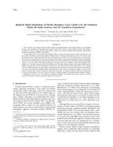
FIG. 6. As for Fig. 4 but comparing accretion parameterizations.

slightly larger (by a few percent) than the center of the smallest radius bin classified as drizzle.

b. Accretion Accretion rates were derived in the same method as autoconversion rates but by integration of (3). Accretion rates are compared in Fig. 6. The parameterization schemes tend to perform better than for autoconversion rate, with T⫹C being the least biased. Biases in the other schemes do not exceed 70%, which is encouraging. For reasons mentioned above, the accretion rates are likely to be accurate to no better than a factor of 2. Maximum averaging biases are also of this magnitude, but in most cases they are small (see appendix). The

formulations for accretion rate all have similar dependencies upon cloud and drizzle liquid water content. The rate of loss of cloud droplets is parameterized in K⫹K by assuming that all collected drops (through both autoconversion and accretion) have a size equal to the mean volume radius of the cloud droplets. Such rates are important for the investigation of aerosol scavenging effects and the associated transition from a polluted to a clean boundary layer. We test this by comparison with the rate of cloud droplet loss using the SCE integrations. It should be noted that K⫹K does not take into account self-collection, that is, the loss of drops by coalescing cloud drops that do not produce a drizzle drop. Results suggest, however, that although

3044


VOLUME 62

cloud droplet loss by self-collection is often comparable to or larger than that by autoconversion, it is accretion that tends to dominate the removal of cloud drops. Thus, the self-collection contribution to the overall cloud droplet loss rate is small. We use the autoconversion and accretion rates derived using the SCE integrals to avoid the aliasing of biases that have been alreadydiscussed in these rates, and concentrate only on the parameterized cloud droplet loss rates. Figure 7a shows the rates derived from the SCE method against the parameterization. For SCE-estimated droplet loss rates higher than around 100 m⫺3 s⫺1 the rates in most cases agree to within a factor of 2. For lower loss rates the parameterization tends to overestimate the rate of droplet loss. However, a droplet loss rate of 100 m⫺3 s⫺1 means that in one hour only 0.36 cloud droplets are lost to autoconversion/accretion, which is rather insignificant. We also compare cloud droplet loss rates with those from BEH, which has separate rates for the loss due to autoconversion, accretion, and self-collection. The droplet loss rates for autoconversion and accretion rates are presented in BEH as a function of the mass autoconversion and accretion rates and, as with the K⫹K comparison, we use the SCE-derived values. We compare the total rate of cloud droplet loss in Fig. 7b for BEH. As with K⫹K, these compare favorably at larger rates, and there is a tendency for overprediction especially at the smaller rates. Neither T⫹C or KES include terms to account for removal of cloud droplets due to the coalescence mechanism.

c. Sedimentation Parameterization of the drizzle process requires expressions for the rate at which the droplet population sediments. Given that the drizzle droplet population is well modeled using an exponential distribution, parameterization of drizzle drop sedimentation rates will require specification of the rate at which both the drop number and a second moment of the distribution falls (i.e., a two-moment parameterization of the DDSD). The mass fall rate is simply the precipitation rate R defined as R ⫽ Rmass ⫽

4␲␳w 3

冕

⬁

wT r3n共r兲 dr,

共8兲

0

and the number fall rate is Rnumber ⫽

冕

FIG. 7. Comparison of combined autoconversion/accretion rate of loss of cloud droplets derived from the observed droplet size distributions (abscissa) with those parameterized (ordinate) assuming that all collected drops have the size of the mean volume radius of the cloud drops r␷.

⬁

wT n共r兲 dr.

共9兲

0

We have plotted the mass and number fall speeds as parameterized using K⫹K against the observed ones in

Fig. 8. In most cases these agree to within a factor of 2. Note that in all cases the observed fall rates include the contribution from the exponential extrapolation at large sizes. The K⫹K precipitation rates are generally slightly lower and the number rates slightly higher than those from the observations. The cause of these differences is not clear but may include differences in the drop terminal velocity relationships used in both cases.

SEPTEMBER 2005

WOOD

3045

files of autoconversion and accretion. To construct the plot we use the autoconversion and accretion rates derived from the observations (sections 3a,b). For each flight we normalize the autoconversion rates by the cloud mean values and then bin the data from all the flights into normalized height bands. Autoconversion rate increases rapidly with height in the cloud. A linear increase of cloud liquid water content with height, a constant droplet concentration, and autoconversion rates that depend upon qL to some power a, leads to curves of the form shown by the dashed lines, for values of a ⫽ 1, 2, 3, 4. ⌻he observed increase in autoconversion rate with z is consistent * with 2 ⬍ a ⬍ 3 discussed in section 3a. Accretion rates peak farther down in the cloud at around z ⫽ 2/3. The * lower panels in Fig. 9 show the relative contribution to the total rate of increase of drizzle liquid water content (autoconversion ⫹ accretion) from the two processes. Accretion dominates the production of qL,D throughout most of the cloud. Autoconversion only becomes a significant process in the upper 20% of the cloud. Even in these upper levels accretion still plays a significant role. Because autoconversion rates are significant only in a thin layer of cloud, its parameterization in numerical models with coarse vertical resolution is likely to be particularly problematic and may suggest why some of the commonly used parameterizations require considerable tuning when used in such models (Pincus and Klein 2000; Rotstayn 2000).

5. Radar reflectivity–precipitation rate relationships

FIG. 8. (a) Mass and (b) number of fall rates as defined in Eqs. (8) and (9) compared with those using the parameterization of Khairoutdinov and Kogan (2000). Dashed lines show perfect agreement; dotted lines show factor of 2 errors.

4. Relative roles of autoconversion and accretion The relative importances of autoconversion and accretion in determining the increase in drizzle liquid water content is an interesting issue that has received little specific attention in the literature. Results presented in section 3a suggest that autoconversion rates depend strongly upon the liquid water content, and therefore height in the cloud. Accretion rates depend not only upon cloud (r ⬍ 20 ␮m) microphysical parameters (Nd, qL), but also upon the drizzle liquid water content, which has a broad peak in the center of the cloud (see Part I). Figure 9 shows a composite of normalized pro-

With the increasing use of radars to measure stratocumulus cloud and precipitation properties from both the ground (e.g., Frisch et al. 1995; Yuter et al. 2000) and from space (e.g., the upcoming CloudSat mission), there is a need to understand the relationships between parameters measured with the radar and physically significant cloud properties. Precipitation rate is one of the key properties that has great implications for the hydrological cycle and for the dynamics of the boundary layer. It is therefore not surprising that relationships between radar reflectivity and precipitation rate (Z–R relationships) have been most scrutinized, albeit in most cases for clouds with significantly higher precipitation rates than are found in stratocumulus cloud (e.g., Stout and Mueller 1968). The measurements presented in this study offer the opportunity of investigating such relationships in stratocumulus cloud. We present measurements from all in-cloud levels in all flights in Fig. 10, in the form of a comparison of the

3046


VOLUME 62

FIG. 9. Composite profiles from all flights of (a) autoconversion and (b) accretion rate normalized with the flight mean in each case, and the fraction of total drizzle liquid water content production rate (autoconversion ⫹ accretion) contributed by (c) autoconversion and (d) accretion. In all plots solid circles are median values for each height bin; dashed lines show 25th and 75th percentiles. The dashed curves in (a) show the autoconversion rate expected for a cloud with a linear increase in cloud liquid water content with height and where autoconversion depends upon liquid water content to the power a, with a ⫽ 1, 2, 3, 4.

total dBZ calculated from the extrapolated exponential (60 ␮m ⬍ r ⬍ ⬁, ordinate) and from the uncorrected 2D-C data (abscissa). The dashed line shows exact agreement and the dotted lines represent the extrapolated exceeding the data by 2.5, 5, and 7.5 dBZ. It is clear that for the majority of flights the differences are small (less than 2.5 in many cases). However, there is a tendency for poorer agreement at larger values of dBZ, that is, for the heavier drizzle cases. Levels below cloud are not included because evaporation of the smaller droplets tends to result in nonexponential size distributions. We did not include flight A641 in this comparison

because it contained low amounts of drizzle droplets and n(r) at large drop size was noisy and not well modeled with an exponential. We do not show the comparison between precipitation rates but the behavior is qualitatively similar to that for dBZ. The fractional increase in Z from the data to the exponential extrapolation is a factor of 1.0 to 3.0 times the fractional increase in R. Because the value of this factor is positively correlated with high values of R, there are important consequences for the true Z–R relationships in drizzling stratocumulus. Values of R and Z are derived for the DDSD over

SEPTEMBER 2005

WOOD

FIG. 10. Reflectivity factor dBZ derived using droplets with radii larger than 60 ␮m for data values (abscissa) and for the fitted exponential distributions extrapolated to r ⫽ ⬁ (ordinate). In most cases there is only a small difference between the two values, indicating that the 2D-C sample volume is sufficiently large enough to account for significant contributions to reflectivity from all droplet sizes. However, in A644 there are differences of at least 10 dBZ in some cases, which arise because drops larger than those measured using the 2D-C are contributing significantly to the reflectivity.

the size range r ⬎ 20 ␮m in two ways. The first method is a direct calculation from the measured DSD giving values Rdata and Zdata. The second uses the exponentially fitted DSD for r ⬎ 60 ␮m drops and the measured values for r ⱕ 60 ␮m, giving values Rexp and Zexp. For flight A641 we use only the measured DSD for reasons mentioned above, so the two methods yield the same values of Z and R. Least squares fitting is used to obtain the parameters a and b in the relationship Z ⫽ aRb. Table 2 shows the values of a and b for the fits, along with the estimated errors (2-␴ level) and the regression coefficient r2. The most important difference between the relationships is that the exponent b is larger for the extrapolated data (b ⫽ 1.18) than the measured data (b ⫽ 1.04). This is a direct result of there being larger

3047

fractional increases in Z than in R for the extrapolated distributions compared with the measured ones. These values of a and b for the extrapolated distributions Z–R relationship compare well with those derived from millimeter cloud radar data taken in drizzling stratocumulus over the southeast Pacific Ocean (Comstock et al. 2004), suggesting that a single Z – R relationship may suffice to detect drizzle from a stratiform marine boundary layer cloud. Figure 11 shows the Zexp–Rexp relationship for all in-cloud cases. The value of r2 for the log–log fit is 0.89. These results suggest that, although there is a good correlation between radar reflectivity and precipitation rate, the relationship is not a unique one. Additional information about the drop size distribution will improve the relationship. Retrievals of precipitation rate from radar reflectivity alone will incur considerable error (Fig. 11), possibly as much as a factor of 2 or 3 in precipitation rate. With additional information, this error can be approximately halved.

6. Discussion and conclusions We have investigated some aspects of the sizeresolved drizzle microphysics using 12 flights into stratocumulus clouds. The drizzle drop size distribution (DDSD) is found to be well represented using either a truncated exponential or a truncated lognormal distribution, and the former has been used to correct for the poor sampling of drops larger than r ⬃ 200 ␮m. Values of the higher moments of the DDSD necessary to derive radar reflectivity and rain rate are, in some cases,

TABLE 2. Details of the Z–R relationships derived from the measured and extrapolated size distributions. Units are mm6 m⫺3 (reflectivity) and mm h⫺1 (precipitation rate) to retain consistency with other studies. Numbers in parentheses indicate 2-␴ errors in a and b (percentage for a, absolute for b). Relationship Zdata ⫽ aP Zexp ⫽ aP

b data b exp

a

b

r2

6.0 (36.8%) 12.4 (51.6%)

1.04 (0.07) 1.18 (0.10)

0.89 0.88

FIG. 11. (a) Derived reflectivities Zexp plotted against precipitation rates Rexp for all the in-cloud extrapolated distributions. The dotted line represents the best fit power law with parameters given in Table 2. Symbols as for Fig. 10.

3048


found to be biased by the poor sampling, particularly at higher rain rates. Values of autoconversion, accretion, and sedimentation rates are estimated using integration of the SCE from the cloud and drizzle DSDs and compared to those from five widely used parameterizations. Autoconversion rates compare most favorably with a modified version of Liu and Daum (2004), whereas accretion rate formulations all show good agreement with data, there being less variation in the parameterizations. The data are consistent with a power 2–3 dependency upon cloud liquid water content. We also found a strong and statistically significant dependence of the autoconversion rate upon cloud droplet concentration Nd, with autoconversion rate decreasing markedly with increasing Nd. A doubling of Nd leads to a decrease in autoconversion rate of between 2 and 4, with the range in this estimate related to uncertainties in the relationship between autoconversion and Nd. This suggests a strong role for cloud microphysical properties in the production of drizzle and supports the hypothesis that drizzle can be suppressed in clouds with high cloud droplet concentration. Modeling is required to investigate the dynamical and thermodynamical feedbacks associated with suppression (e.g., Ackerman et al. 2004). It is found that the accretion rate dominates the production of drizzle liquid water throughout most of the cloud with autoconversion being dominant at cloud top only. The production of new drizzle drops is dominant at cloud top. Radar reflectivity–rain rate (Z–R) relationships are found to be affected by the sampling problems discussed above. With data corrected for the sampling problems, we find an exponent b ⬃ 1.2 that is smaller than those commonly found in heavier rain b ⬃ 1.5. This relationship is explored further in Comstock et al. (2004) and is suggestive of a stronger control on rain rate by variations in number concentration of drizzle drops and less control by the size of drizzle drops, compared to heavier rain. These relationships should prove useful when designing drizzle retrieval methods from surface and satellite radars. Acknowledgments. The author wishes to thank the staff of the Meteorological Research Flight and the C-130 aircrew and groundcrew for their dedication to collecting the data presented in this study. I am grateful to colleagues in the Met Office and elsewhere for discussions that aided the research presented in this paper. I thank Andreas Bott for provision of the numerical code to solve the SCE and Jean-Louis Brenguier, Gabor Vali, and an anonymous reviewer for their insightful and constructive reviews.

VOLUME 62

APPENDIX Effect of DSD Averaging on Autoconversion and Accretion Rates The use of layer average rather than instantaneous spectra has the potential to induce a bias in the estimation of the layer mean autoconversion rate because in general, F [n(r)] ⫽ F [n(r)], where F is any function, such as the autoconversion rate, that depends nonlinearly upon the DSD. We estimate the potential magnitude of these biases for the autoconversion rate using 1-km average DSDs from a selection of straight and level runs with lengths between 20 and 60 km. For each run we compare the autoconversion rate Aens estimated using the ensemble DSD for the entire run with the mean autoconversion rate Amean of the 1-km estimates (Fig. A1). The median value of Aens/Amean is 0.96 with 10th and 90th percentiles of 0.56 and 1.28. This suggests that the use of layer means can lead to considerable biases of nearly a factor of 2, but that, perhaps surprisingly, both underestimation and overestimation by the ensemble DSD is possible, and the net effect turns out to be a relatively small bias. The bias characteristics do not appear to differ markedly at low or high autoconversion rates. In the types of stratocumulus studied here, the results suggest that the maximum error in the estimate of the mean autoconversion rate when a layer mean DSD is used is almost a factor of 2. That Aens/Amean can be both less than and greater than unity is worthy of closer examination. To demonstrate how this can happen, we consider two hypotheti-

FIG. A1. Comparison of autoconversion rate derived from the ensemble DSD for entire 20–60-km straight and level runs (abscissa), against the mean of the autoconversion rates calculated for each 1-km subsection of the run.

SEPTEMBER 2005

WOOD

cal extreme cases. First, consider a variable cloud in which the liquid water content is modulated entirely by changes in cloud droplet number concentration rather than mean droplet size. The DSD can be written as n(r) ⫽ Nd f(r), where f(r) is a fixed function of droplet radius in the cloud. The autoconversion integral (2) yields a local autoconversion rate proportional to N2d. Thus, in 2 this case, Aens /Amean ⫽ N d /N 2d ⫽ [1 ⫹ (␴N /Nd)2]⫺1 ⬍ 1, and the ensemble underestimates the mean autoconversion. For the second case, we assume that at each location in the cloud the DSD is a Dirac delta function (i.e., monodisperse) and that the droplet concentration is fixed so that liquid water variability is related only to changes in mean droplet size. In this case, Amean ⫽ 0 because the collection kernel K(r, r ⬘) ⫽ 0 for r ⫽ r ⬘. Because the ensemble DSD is broad, Aens ⬎ 0, so the ensemble in this case overpredicts the autoconversion rate. While neither of these examples are representative of any real cloud, they demonstrate that the relative variability of cloud droplet concentration and mean droplet radius, and the degree to which these variables are correlated in real clouds will determine whether the layer mean DSD will underestimate and overestimate the true layer mean autoconversion rate. Similar biases occur in accretion rates. In this case, biases arise only if there is a nonzero spatial correlation between cloud and drizzle liquid water contents because the accretion rate is nearly proportional to their product. We estimate that the ratio of ensemble to mean accretion has a median of 0.97 with 10th and 90th percentiles of 0.70 and 1.08. In the extreme cases, the ensemble DSD can underestimate the mean autoconversion by up to a factor of 2 or overestimate it by 20%, but more commonly the biases are much less than this, and do not exceed the uncertainties related to the collection kernel and DSD measurement error. REFERENCES Ackerman, A. S., M. P. Kirkpatrick, D. E. Stevens, and O. B. Toon, 2004: The impact of humidity above stratiform clouds on indirect aerosol forcing. Nature, 432, 1014–1017. Austin, P., Y. Wang, R. Pincus, and V. Kujala, 1995: Precipitation in stratocumulus clouds: Observations and modeling results. J. Atmos. Sci., 52, 2329–2352. Baker, M. B., 1993: Variability in concentrations of cloud condensation nuclei in the marine cloud-topped boundary layer. Tellus, 45B, 458–472. Baumgardner, D., B. Baker, and K. Weaver, 1993: A technique for measurement of cloud structure on centimeter scales. J. Atmos. Oceanic Technol., 10, 557–565. Beard, K. V., and H. T. Ochs, 1993: Warm-rain initiation: An overview of microphysical mechanisms. J. Appl. Meteor., 32, 608–625. Beheng, K. D., 1994: A parameterization of warm cloud microphysical conversion processes. Atmos. Res., 33, 193–206. ——, and G. Doms, 1986: A general formulation of collection

3049

rates of cloud and raindrops using the kinetic equation and comparison with parameterizations. Beitr. Phys. Atmos., 59, 66–84. Berry, E. X., and R. L. Reinhardt, 1974: An analysis of cloud drop growth by collection. Part II: Single initial distributions. J. Atmos. Sci., 31, 1825–1831. Bott, A., 1998: A flux method for the numerical solution of the stochastic collection equation. J. Atmos. Sci., 55, 2284–2293. Bretherton, C. S., and Coauthors, 2004: The EPIC 2001 stratocumulus study. Bull. Amer. Meteor. Soc., 85, 967–977. Brown, P. R. A., G. Richardson, and R. Wood, 2004: The sensitivity of large-eddy simulations to the parameterization of drizzle. Proc. 14th ICCP Conf. on Clouds and Precipitation, Bologna, Italy, ICCP, CD-ROM, 174. Comstock, K., S. Yuter, and R. Wood, 2004: Reflectivity and rain rate in and below drizzling stratocumulus. Quart. J. Roy. Meteor. Soc., 130, 2891–2919. Davis, M. H., 1972: Collisions of small droplets: Gas kinetic effects. J. Atmos. Sci., 29, 911–915. Feingold, G., and Z. Levin, 1986: The lognormal fit to raindrop spectra from frontal convective clouds in Israel. J. Climate Appl. Meteor., 25, 1346–1363. Frisch, A. S., C. W. Fairall, and J. B. Snider, 1995: Measurement of cloud and drizzle parameters during ASTEX with a K␣ band Doppler radar and a microwave radiometer. J. Atmos. Sci., 52, 2788–2799. Golovin, A. M., 1963: The solution of the coagulation equation from cloud droplets in a rising air current. Izv. Akad. Nauk. SSSR Ser. Geofiz., 5, 783–791. Hall, W. D., 1980: A detailed microphysical model within a twodimensional dynamic framework: Model description and preliminary results. J. Atmos. Sci., 37, 2486–2507. Hobbs, P. V., 1993: Aerosol–Cloud–Climate Interactions. Academic Press, 235 pp. Hudson, J. G., and S. S. Yum, 2001: Maritime–continental drizzle contrasts in small cumuli. J. Atmos. Sci., 58, 915–926. Jonas, P. R., 1972: The collision efficiency of small drops. Quart. J. Roy. Meteor. Soc., 98, 681–683. Jones, A., D. L. Roberts, M. J. Woodage, and C. E. Johnson, 2001: Indirect aerosol forcing in a climate model with an interactive sulphur cycle. Hadley Centre Tech. Note HCTN-25, Meteorological Office, 34 pp. Kessler, E., 1969: On the Distribution and Continuity of Water Substance in Atmospheric Circulations, Meteor. Monogr., No. 32, Amer. Meteor. Soc., 84 pp. Khairoutdinov, M., and Y. Kogan, 2000: A new cloud physics parameterization in a large-eddy simulation model of marine stratocumulus. J. Atmos. Sci., 57, 229–243. Liu, Y., and P. H. Daum, 2004: Parameterization of the autoconversion process. Part I: Analytical formulation of the Kesslertype parameterizations. J. Atmos. Sci., 61, 1539–1548. ——, ——, and R. McGraw, 2004: An analytical expression for predicting the critical radius in the autoconversion parameterization. Geophys. Res. Lett., 31, L06121, doi:10.1029/ 2003GL019117. Menon, S., and Coauthors, 2003: Evaluating aerosol/cloud/ radiation process parameterizations with single-column models and Second Aerosol Characterization Experiment (ACE2) cloudy column observations. J. Geophys. Res., 108, 4762, doi:10.1029/2003JD003902. Pawlowska, H., and J.-L. Brenguier, 2003: An observational study of drizzle formation in stratocumulus clouds for general cir-

3050


culation model (GCM) parameterizations. J. Geophys. Res., 108, 8630, doi:10.1029/2002JD002679. Pincus, R., and S. A. Klein, 2000: Unresolved spatial variability and microphysical process rates in large scale models. J. Geophys. Res., 105, 27 059–27 066. Pruppacher, H. R., and J. D. Klett, 1997: Microphysics of Clouds and Precipitation. Kuwer Academic Publishers, 976 pp. Rotstayn, L. D., 1997: A physically based scheme for the treatment of stratiform clouds and precipitation in large-scale models. I: Description and evaluation of the microphysical processes. Quart. J. Roy. Meteor. Soc., 123, 1227–1282. ——, 2000: On the “tuning” of autoconversion parameterizations in climate models. J. Geophys. Res., 105, 15 495–15 507. ——, and Y. Liu, 2005: A smaller global estimate of the second aerosol effect. Geophys. Res. Lett., 32, L05708, doi:10.1029/ 2004GL021922. Stephens, G. L., and Coauthors, 2002: The CloudSat mission and the EOS constellation: A new dimension of space-based observations of clouds and precipitation. Bull. Amer. Meteor. Soc., 83, 1771–1790. Stevens, B., R. L. Walko, W. R. Cotton, and G. Feingold, 1996: The spurious production of cloud-edge supersaturations by Eulerian models. Mon. Wea. Rev., 124, 1034–1041. Stout, G. E., and E. A. Mueller, 1968: Survey of relationships between rainfall rate and radar reflectivity in the measurement of precipitation. J. Appl. Meteor., 7, 465–474. Tripoli, G. J., and W. R. Cotton, 1980: A numerical investigation

VOLUME 62

of several factors contributing to the observed variable density of deep convection over south Florida. J. Appl. Meteor., 19, 1037–1063. Tzivion, S., G. Feingold, and Z. Levin, 1987: An efficient numerical solution to the stochastic collection equation. J. Atmos. Sci., 44, 3139–3149. vanZanten, M. C., B. Stevens, G. Vali, and D. Lenschow, 2005: Observations of drizzle in nocturnal marine stratocumulus. J. Atmos. Sci., 62, 88–106. Wilson, D. R., and S. P. Ballard, 1999: A microphysically based precipitation scheme for the UK Meteorological Office unified model. Quart. J. Roy. Meteor. Soc., 125, 1607–1636. Wood, R., 2000: Parametrization of the effect of drizzle upon the droplet effective radius in stratocumulus clouds. Quart. J. Roy. Meteor. Soc., 126, 3309–3324. ——, 2005: Drizzle in stratiform boundary layer clouds. Part I: Vertical and horizontal structure. J. Atmos. Sci., 62, 3011–3033. ——, and P. Blossey, 2005: Comments on “Parameterization of the autoconversion process. Part I: Analytical formulation of the Kessler-type parameterizations.” J. Atmos. Sci., 62, 3003– 3006. Yuter, S. E., Y. L. Serra, and R. A. Houze Jr., 2000: The 1997 Pan American climate studies tropical eastern Pacific process study. Part II: Stratocumulus region. Bull. Amer. Meteor. Soc., 81, 483–490.