This is authors' version of the paper of Computer Standards & Interfaces vol. 33, no. 2, 2011, pp. 182-190
doi:10.1016/j.csi.2010.06.010
DSP instrument for transient monitoring Tomasz Tarasiuk, Mariusz Szweda Gdynia Maritime University, Department of Ship Electrical Power Engineering, Morska 83, 81-225 Gdynia, Poland, phone: (+48 58) 690-14-14, fax: (+48 58) 620-67-01, e-mail:
[email protected],
[email protected]
Ab st ra c t - This paper consists of two parts oriented toward transient detection and monitoring in electric power systems. Firstly, a problem of frequency characteristic of real impulses is considered. Parameters of the selected transient and notching disturbances are determined after extracting disturbances by pass-band filters with various cut-off frequencies. Further, results of wavelet transform application for estimation of selected disturbances are presented. Secondly, basic features of the prototype of original multi-parameter instrumentation for power quality assessment are shown and its transient monitoring capabilities are discussed on the basis of laboratory research of the testing signals. This new measurement instrument utilizes the digital signal processor (DSP) technique. Keywords: power quality, transients, wavelet transform, digital signal processors I. Introduction According to IEC Standard 61000-4-30 the term power quality means “characteristic of the electricity at a given point on an electrical system, evaluated against a set of reference technical parameters” [27]. The set of reference parameters consists of various electromagnetic phenomena, but usually relatively low frequency phenomena are considered up to 9 kHz [6-8, 28]. However, an interest in higher frequency phenomena is growing lately, despite problems with their capturing and assessment [7]. In this respect, the most often analyzed are transients and notching disturbances [1-4, 7, 10-12, 15, 17, 25]. The terms “transient” and “notching” were defined in IEEE Standard 1159-1995 [29]. According to the standard transients can be divided into two groups: impulsive and oscillatory. The former term means “a sudden non-power frequency change in steady-state conditions of voltage, current or both, that is unidirectional in polarity” [29]. The latter term means “voltage or current whose instantaneous value changes polarity rapidly” [29]. These disturbances usually contain high frequencies (from a few hundred hertz up to a few MHz) and their duration varies from below 50 ns up to a few dozen ms [29]. A similar kind of disturbance is notching. This is “a periodic voltage disturbance” caused by operation of power electronics
This is authors' version of the paper of Computer Standards & Interfaces vol. 33, no. 2, 2011, pp. 182-190
doi:10.1016/j.csi.2010.06.010
devices [29]. Frequency components characterizing notching can be quite high, similarly as in the case of transients. Sometimes this kind of disturbance is called “periodic transient” [4]. The characteristics of discussed disturbances have an enormous impact on required parameters of the measurement instrumentation. Frequency components associated with transient and notching disturbances are significantly higher than usually covered by power quality analyzers. They require a wide bandwidth of measurement circuit and high sampling frequency [7], if a transient monitoring is to be carried out by fast analog-to-digital conversion. Moreover, due to relatively high magnitude of transients, a sufficient input range of measurement instrument is required. But typical power quality analyzers are optimized for measurement of components up to the 40th or 50th harmonic (maximum 3 kHz in the case of 60 Hz systems) or sometimes up to 9 kHz. The latter value results directly from IEC standard 61000-4-7 [28]. According to this standard the sampling frequency of a measuring device should be sufficient for analysis of power quality disturbances up to 9 kHz. Obviously, sampling frequency sufficient for measurement of low-frequency components up to 9 kHz would be insufficient for transient and notching analysis. So, the proper transient assessment would require dedicated instrumentation. Nevertheless, many multi-parameter power quality analyzers are capable of transient analysis. However, their data sheet can cause some confusion and methods of detecting and characterizing transients are often undisclosed [7]. For example, sampling frequencies declared by various developers of power quality analyzers are equal to e.g. 38.4 kHz [5], 50 kHz [16] or 200 kHz [26]. Obviously, these sampling frequencies are insufficient for covering all notching and transients as defined in the IEEE standard [29], but would they be sufficient for common ones? In the first part of this paper results of analysis of frequency characteristics of three real examples are presented and discussed. Detection of the analyzed disturbances is a separate problem, since their typical duration is very short, usually below one cycle of the fundamental wave [9]. It has to be underlined that a proper evaluation of many transient or notching parameters requires determining the exact beginning and ending of discussed disturbances. Generally, the transient detection methods are based either on the original signal waveform or extracted transient [7]. In the latter case some kind of high-pass filtration is required. For example, in the case of the measurement instrument described in Ref. [16], a 6th order IIR filter was applied, with cutoff frequency 100 Hz. Next, mathematical morphology was used for signal processing. The tool was also discussed in Ref. [15]. However, it seems that the most popular tool for transients and notching analysis is
This is authors' version of the paper of Computer Standards & Interfaces vol. 33, no. 2, 2011, pp. 182-190
doi:10.1016/j.csi.2010.06.010
discrete wavelet transform DWT [1-4, 7, 17]. Application of DWT does not require high-pass filtering. But the number of implemented decomposition stages has to be determined. In some respect, it can be treated as a proper choice of the cut-off frequency of high-pass filter. The exact detection of transient beginning and ending can be carried out by various methods. They involve a comparison of respective original signal samples or extracted transient with user-defined thresholds as well as comparison of the waveform of two adjacent cycles of the analyzed signal (comparison with the pre-event steady-state waveform) [7, 11]. Summing up, when designing a feasible transient monitoring instrument, especially its bandwidth has to be carefully considered. Further, methods of transient extraction and description should be chosen. The second part of this paper presents the hardware structure, applied methods and research results of the prototype of new instrumentation for transient monitoring. In fact, the discussed device is a multiparameter power quality analyzer with transient monitoring capabilities. II. Transient indices The transient description is usually based on the magnitude and duration [7]. Transient magnitude assessment can be based on its absolute value, but sometimes the extracted disturbance peak-to-peak value is considered [1, 10]. In the case of the notching phenomenon, a notch area is taken into account [30]. A measure of transient severity is transient energy [7]. It can be defined as follows [7, 23]:
Et =
t2
∫
t1
ut2 ( t )dt ≈ 1 ⋅ fs
kt 2
∑ u k2
(1)
k t1
where: ut(t) – impulse signal, t1 – start of impulse, t2 – end of impulse, fs – sampling frequency, kt1 – first sample of the transient impulse, kt2 – last sample of the transient impulse. Most power quality parameters are calculated on the basis of ten or twelve cycles of input signal, depending on analyzed system rated frequency, 50 Hz or 60 Hz respectively [27-28]. In order to avoid excessive data in the case of multiple transients or notching, the below-described prototype of power quality analyzer determines transient indices every ten cycles (it was designed for 50 Hz systems). Finally, for each basic measurement window successive transient indices are registered in the internal RAM memory of the instrument or transferred to an external device (e.g. PC computer):
This is authors' version of the paper of Computer Standards & Interfaces vol. 33, no. 2, 2011, pp. 182-190
doi:10.1016/j.csi.2010.06.010
−
maximum peak-to-peak value Vp-p of singular transient during the basic measurement window (approximately 200 ms),
−
maximum energy maxEn of singular transient during the basic measurement window,
−
number of transients registered during measurement window,
−
combined duration Σtd of all transients registered during the basic measurement window,
−
combined energy ΣEn of all transients registered during the basic measurement window. III. Research of frequency characteristics of the real transients A. Signals under research
The phenomena discussed in this paper are hard to detect and register due to limited capabilities of typical measurement devices for power quality phenomena monitoring. In particular, a short-duration impulse is especially hard to evaluate, since its high frequency components will be removed by an anti-aliasing filter, which has an adverse influence especially for transient magnitude assessment [7]. Therefore, the number of real transients and their characteristics described in the literature is limited [7]. The authors of this paper carried out a study of power quality in electric power networks (mainly ship networks) for quite a few years. During this time dozens of hours of power signals were registered with various sampling frequencies. Fortunately, during this research some examples of transient and notching were registered. The examples selected for this paper are shown in Fig. 1. They were registered by means of DAQ PCI703-16/A Eagle Technology equipped with a 14-bit A/D converter. Isolation amplifiers ISO 124 of Burr Brown were used as well. The maximum bandwidth of these amplifiers was equal to 50 kHz. So, the analysis presented below is valid for this particular frequency band. Applied sampling frequency was equal to 150375 Hz. a). 1000 800 600 400 u(t) [V]
200 0 -200 -400 -600 -800 -1000 0
5
10
15 time [ms]
20
25
30
This is authors' version of the paper of Computer Standards & Interfaces vol. 33, no. 2, 2011, pp. 182-190
doi:10.1016/j.csi.2010.06.010
b).
800 600 400 200
101V
u(t) [V]
0 -200 -400 -600 -800 -1000 -1200
-1218V
-1400 0
5
10
15
20
25
30
time [ms]
c). 800 600 400
u(t) [V]
200 0 -200 -400 -600 -800 0
5
10
15
20
25
30
35
40
time [ms]
Fig. 1. Examples of transient and notching registered in ship networks: a) notching (further marked as notch), b) impulsive transient (marked as imp) and c) oscillatory transient (marked as osc). It should be added that the example presented in Fig. 1b is designated as an impulsive transient, although it was bidirectional in polarity. This is for reasons of simplification, since in practical terms the transient is a single triangle impulse. B. Pass-band filtration by means of IIR filters with various cut-off frequencies The analyses of discussed examples consisted in calculation of their peak-to-peak magnitudes and energies over various frequency sub-bands in the range from 200 Hz to 50 kHz. Namely, prior to determining the phenomena parameters the pass-band filtering was applied. There were two stages of research. Firstly, the research consisted in calculation of disturbances’ energy and magnitude as a function of upper cut-off frequency changes of used filter with constant lower cut-off frequency equal to 200 Hz. Secondly, it consisted in changing a lower cut-off frequency of band-pass filter with constant upper cut-off frequency equal to 50 kHz. The results are presented in relation to respective values
This is authors' version of the paper of Computer Standards & Interfaces vol. 33, no. 2, 2011, pp. 182-190
doi:10.1016/j.csi.2010.06.010
calculated for the maximum considered frequency band 200-50000 Hz. It means that the value calculated for the whole frequency band is 100%. a). 120
b). 120
100 100
Amplitude [%]
Energy [%]
80
60
40
80
60
40
notch imp osc
20
notch imp osc
20
0
0
0
5000
10000
15000
20000
25000
30000
35000
40000
45000
50000
0
5000
10000
15000
20000
f [Hz]
30000
35000
40000
45000
50000
f [Hz]
upper cut-off frequency of band-pass filter
upper cut-off frequency of band-pass filter
c). 120 notch imp osc
100
d) 120 .
Amplitude [%]
60
40
notch imp osc
100
80 Energy [%]
25000
80
60
40
20
20
0
0
0
5000
10000
15000
20000
25000
30000
35000
40000
f [Hz]
lower cut-off frequency of band-pass filter
45000
50000
0
5000
10000
15000
20000
25000
30000
35000
40000
45000
50000
f [Hz]
lower cut-off frequency of band-pass filter
Fig. 2. Results of analysis of selected disturbances after band-pass filtering with various corner frequencies: a) – b) values of impulse energy and magnitude measured with constant lower cut-off frequency of band-pass filter equal to 200 Hz and various upper cut-off frequencies; c) – d) values of impulse energy and magnitude measured with constant upper cut-off frequency of band-pass filter equal to 50 kHz and various lower cut-off frequencies. It is discernible that the wrong choice of frequency band has an adverse influence on the results of evaluation of selected disturbance parameters. For instance, imp transient requires analysis over a wider frequency band than the band used during the described research. In particular, the upper limit of the frequency band should be much higher than the cut-off frequency of the applied anti-aliasing filter, which equals 50 kHz. But it seems that a lower limit of the analyzed frequency band equal to 10 kHz should be sufficient. In the case of the other two examples a frequency band up to 5-6 kHz is sufficient for proper evaluation of parameters of such disturbances as notching and low frequency oscillatory transient. But quite low
This is authors' version of the paper of Computer Standards & Interfaces vol. 33, no. 2, 2011, pp. 182-190
doi:10.1016/j.csi.2010.06.010
frequencies should be included in analysis of these disturbance parameters. These two categories of transients and notching are the most frequently encountered in ship networks C. Wavelet decomposition It was mentioned above that there are a few methods for dealing with the discussed phenomena. However, it seems that the most popular tool is DWT. Fortunately, the DWT has some distinct advantages. It can be used concurrently for data compression [14, 18] or it diminishes the demand for DSP resources, by improving performance of methods of assessment of other parameters. In Ref. [19] the original method of combined application of DWT and Fourier transforms for harmonics measurement was described. In short, the method consists in use of wavelet coefficients representing lower frequencies as input series for various methods of calculation of coefficients in Fourier series. Since the wavelet coefficients are decimated after each decomposition stage, this method results in a decrease of overall computational complexity. Further, the method enables saving needed RAM memory. Transients usually contain high frequency components from a few hundred Hz up to a few MHz but their duration is up to 50 ms [29]. In real cases, the transient duration is even shorter [9]. During the abovementioned research, all observed transients lasted no longer than half a cycle of the fundamental wave. According to IEC Standard 61000-4-7, low frequency phenomena should be analyzed on the basis of 10/12 ( for harmonics and interharmonics) or 5/6 cycles (for components above the harmonic frequency range, up to 9 kHz) [28]. So, information about low frequency components must be preserved for approximately 100 ms or 200 ms. It would be an enormous burden in the case of high sampling frequencies required for transient analysis, if original signal samples were stored. Fortunately, wavelet coefficients are decimated after each decomposition stage and only the coefficients representing lower frequencies should be preserved for the whole measurement window for measurement of low frequency parameters. Then, the wavelet coefficients representing different frequency bands can be preserved for different time intervals. This results in saving RAM memory [20]. For example, in the case of the new instrumentation described in the following section, RAM memory needed for data storage was reduced five-fold. The device operates with constant sampling frequency equal to 148917.8 Hz. Other possible DWT applications concern fundamental frequency estimation [21], rough assessment of waveform distortions and fast detection of atypical harmonics fluctuations [20] as well as whole signal rms value calculation [20, 24].
This is authors' version of the paper of Computer Standards & Interfaces vol. 33, no. 2, 2011, pp. 182-190
doi:10.1016/j.csi.2010.06.010
Summing up, DWT can be applied concurrently for: transient and notching monitoring, data compression, decreasing computational complexity of low frequency phenomena assessment and saving needed processor’s RAM. So, the overall performance of the measurement device is improved. Finally, the wavelet decomposition of imp and osc signals are shown in Fig. 3 and Fig. 4 respectively. In
500
0.3 – 0.6 (kHz) 0.6 – 1.2 (kHz) 1.2 - 2.3 (kHz) 2.3 - 4.7 (kHz)
4.7 - 9.4 (kHz) 9.4 - 18.8 (kHz) 18.8 - 37.6 (kHz) 37.6 - 50 (kHz)
particular, Daubechies filters with 10 coefficients were used.
0 -500 500 0 -500 500
0 -500 500 0 -500 0
time (ms)
500 0 -500 500
0 -500 500
0 -500 500 0 -500 0
2.1
time (ms)
2.1
2.3 – 4.7 (kHz)
100 0
1.2 – 2.3 (kHz)
-100 100
0
0.6 – 1.2 (kHz)
-100 100
0
-100 100
100
0
-100 100
0
-100 100
0
-100 100 0.3 – 0.6 (kHz)
4.7 – 9.4 (kHz)
9.4 – 18.8 (kHz) 18.8 – 37.6 (kHz)
37.6 - 50 (kHz)
Fig. 3. Wavelet decomposition of the imp transient into eight frequency sub-bands.
0
-100 0
time (ms)
10
0
-100
0
time (ms)
Fig. 4. Wavelet decomposition of the osc transient into eight frequency sub-bands. The results presented in Fig. 3 confirm previous conclusions that the investigated imp transient contains high frequencies. In practical terms, only the wavelet detail coefficients from first and second
10
This is authors' version of the paper of Computer Standards & Interfaces vol. 33, no. 2, 2011, pp. 182-190
doi:10.1016/j.csi.2010.06.010
decomposition stages are to be used for the case rough assessment. The opposite is true for the oscillatory transient (see Fig. 4). Its rough assessment requires at least seven stages of wavelet decomposition, although detailed analysis of the wavelet coefficients from the fourth to seventh decomposition stage seems enough (only lower frequencies are involved). IV. Estimator-analyzer of power quality A. Hardware structure The prototype of a new kind of power quality estimator-analyzer was designed in Gdynia Maritime University and it was manufactured in co-operation with the Institute of Power Engineering, Gdansk Division, Poland. The device was designed for complex power quality assessment. This means that it is a multi-parameter device. The device determines power quality parameters defined in the respective IEC standards [27, 28] and it has the ability to measure the following parameters [22]: −
voltage r.m.s. value,
−
frequency,
−
unbalance,
−
newly introduced distortion band factors DBF [20],
−
voltage dip estimation (value and duration),
−
harmonic subgroups measurement up to 50th harmonic,
−
interharmonic centered subgroups measurement in the range up to 50th harmonic,
−
sub-harmonic,
−
dc component,
−
groups of high frequency components with bandwidths approximately 200 Hz in the range from 50th harmonic up to 9 kHz,
−
transient and notching detection and assessment,
−
power quality temperature factor for assessment of additional temperature rise of windings of induction motors [13].
The evaluation of so many power quality parameters in real time requires not only appropriate methods but relatively fast processing modules. The core of the device is digital signal processor DSP of SHARC family, ADSP 21364 [31]. All measurement procedures are carried out by the DSP. Additionally, it is
This is authors' version of the paper of Computer Standards & Interfaces vol. 33, no. 2, 2011, pp. 182-190
doi:10.1016/j.csi.2010.06.010
used for analog-digital converter AD 7656 control and data transfer to general purpose processor XC 161. The device’s hardware structure of a single data processing channel is depicted in Fig. 5 and a photograph of its front panel is shown in Fig. 6.
Fig. 5. Hardware structure of data processing channel of the estimator-analyzer; ADSP 21364 – DSP processor, XC 161 – general purpose processor, AD 7656 – analog-digital converter, AD 215 – isolation amplifier, LTC1564 – programmable anti-aliasing filter.
Fig. 6. Front panel of power quality estimator-analyzer [22]. This device lacks the disadvantages of present commercial analyzers. Namely, it enables reliable waveform estimation in the presence of fast harmonic content fluctuation and lack of synchronization of sampling frequency and fundamental one. Simply put, sampling frequency is constant and equal to 148917.8 Hz (cut-off frequency of anti-aliasing filters equals 60 kHz). All components in the low frequency range (up to 9 kHz) are determined on the basis of a rectangular window equal to 10 cycles of input signal. The basic tools for measurement of harmonics and interharmonics are DFT and chirp ztransform CZT. In both cases the wavelet coefficients are utilized in the above-mentioned manner.
This is authors' version of the paper of Computer Standards & Interfaces vol. 33, no. 2, 2011, pp. 182-190
doi:10.1016/j.csi.2010.06.010
The estimator-analyzer possesses the capability of co-operation with a PC computer in real time. Exemplary user’s interface for a PC is presented in Fig. 7. The detailed description of the estimatoranalyzer of power quality is planned in future publications. Currently two pieces of the device have been manufactured.
Fig. 7. Example of user interface of PC for communication with estimator-analyzer of power quality. The importance of proper frequency bandwidth of the measurement instrument for transient assessment was mentioned above. The frequency characteristic of input channel of the discussed instrument has been experimentally determined and it is depicted in Fig. 8. 10
magnitude p.u. [dB]
0 -10 -20 -30 -40 0
20
40
60
80
100
frequency [kHz]
Fig. 8. Frequency characteristic of chosen input channel of the estimator-analyzer.
This is authors' version of the paper of Computer Standards & Interfaces vol. 33, no. 2, 2011, pp. 182-190
doi:10.1016/j.csi.2010.06.010
B. Methods The first task of transient and notching analysis is to detect each singular impulse, especially to determine the start and end point of the impulse. The DWT is used for transient detection in the case of the discussed device (Daubechies filters with 10 coefficients). Seven wavelet decomposition stages are utilized. For detection of the start and end points of transient disturbances the following formula has been applied [23]:
( sk − sk −1 〉 p1) ∨ ( sk 〉 p 2)
(2)
where: sk - k-sample of extracted transient signal, p1, p2 - threshold values. If condition (2) has logical value equal to "true", it means the occurrence of an impulse. The simplicity of formula (2) allows easy implementation for fast transient and notching detection with minimum needed computational power of the measurement device. However, the threshold values p1 and p2 have to be chosen carefully [23]. The threshold values were chosen after experimental investigation as:
p1 = 0.2 ⋅ U n p 2 = 0.06 ⋅ U n where: Un – rated input magnitude ( 2 ⋅ 400 V). The lower threshold values led to unnecessary detection and registration of low energy and low magnitude transients during tests carried out in real systems. It should be added that the end of the transient means the last occurrence of the logical value “true” followed by fifteen values of “false”. Taking into account the estimator-analyzer sampling frequency (148917.8 Hz), this means that the minimum possible gap between two consecutive transients is to be 100.7 µs, otherwise the adjacent transients would be detected as a single impulse and treated accordingly.
C. Research results The estimator-analyzer was investigated under laboratory conditions for several testing signals. The experimental research has been carried out using the three-phase programmable power source Chroma 6590 as well as arbitrary waveform generator Agilent 33120A. For this paper’s purpose the results of investigation of a sinusoidal signal with superimposed triangle wave is described. It represents a
(3)
This is authors' version of the paper of Computer Standards & Interfaces vol. 33, no. 2, 2011, pp. 182-190
doi:10.1016/j.csi.2010.06.010
disturbance similar to the real transient presented in Fig. 1b. The Agilent 33120A generator was used for this aim. Since the maximum possible peak-to-peak value of the generated signal was ±10V, the input voltage divider was bypassed, but results of measurements were recalculated according to voltage divider parameters. The exemplary testing signal waveform is depicted in Fig. 9.
u(t) [V]
2
0
-2
-4
0
time [ms]
40
Fig. 9. Waveform of exemplary testing signal; transient duration 752 µs. The results of the research presented in this paper represent measured values of transient parameters as a function of transient fundamental frequency. This frequency can be understood as reciprocal of the impulse duration. The comparison of measurement results of transient parameters listed above (Sec. II) with Agilent 33120A respective setting values is shown in Fig. 10. The values represent mean values of 1000 measurements. It should be added that the setting values were controlled by a Tektronix TDS 420A digital oscilloscope as well.
This is authors' version of the paper of Computer Standards & Interfaces vol. 33, no. 2, 2011, pp. 182-190
doi:10.1016/j.csi.2010.06.010
a)
b) 1000
10000
Results of Measurement Setting values
Results of Measurement
maxEn [V2s]
Vp-p [V]
Setting values
1000
100
10
1
0,1
100
0
10
20
30
40
50
60
70
0
10
20
f [kHz]
c)
40
50
60
70
f [kHz]
d)
10000
100000
Results of Measurement Setting values
Results of Measurement Setting values
Σ td [µs]
1000 2 Σ En [V s]
30
100
10000
1000 10
100
1 0
10
20
30
40
50
60
70
0
10
20
30
40
50
60
70
f [kHz]
f [kHz]
Fig. 10. Comparison of measurement results of respective transient parameters with setting values; a) maximum registered peak-to-peak magnitude Vp-p, b) maximum registered energy maxEn, c) combined energy of all transients during basic measurement window ΣEn, d) combined duration Σtd of all transients during basic measurement window. The measurement results of respective transient parameters for chosen frequencies were also set out in Table 1. The results represent mean values µ, standard deviations σ of 1000 measurements completed by maximum and minimum registered values of respective transient parameters.
This is authors' version of the paper of Computer Standards & Interfaces vol. 33, no. 2, 2011, pp. 182-190
doi:10.1016/j.csi.2010.06.010
Table 1. Results of respective transient parameters measurement
Transient indices Setting values
maxEn [V2s]
ΣEn [V2s]
Σtd [µs]
1004
1102
1038
919.6
672.5
σ
142.7
1.7
2.7
12.8
8.2
max
1074
1105
1043
936.6
688.4
min
651
1096
1031
875.2
642.0
Setting values
106.66
71.07
10.67
4.27
2.13
µ
85.30
67.91
10.63
4.36
1.72
σ
13.86
0.16
0.01
0.10
0.02
max
92.5
68.1
10.65
4.42
1.75
min
50.2
67.2
10.58
3.87
1.64
Setting values
1066.7
710.7
106.7
42.7
21.3
µ
785.4
613.8
106.1
40.9
16.4
σ
11.1
5.97
0.07
0.72
0.19
max
802.1
623.3
106.3
44.0
17.1
min
767.7
605.9
105.7
38.5
15.7
Setting values
10000
6663
1000
400
200
µ
11513
5753
1059
616.4
595.2
σ
3456
24
6
13
12
max
12289
5876
1088
665
638
min
10758
5708
1048
571
557
10
10
10
10
10
µ
21.4
10.13
10
10
10
σ
1.3
0.4
0
0
0
max
25
13
10
10
10
min
18
10
10
10
10
Measured values
Measured values
Measured values
Measured values
Setting values Number of impulses
50 kHz (td=20µs) 1131.4
µ
Vp-p [V]
1 kHz (td=1000µs) 1131.4
Frequency of singular impulse (duration of singular impulse) 1.5 kHz 10 kHz 25 kHz (td=666µs) (td=100µs) (td=40µs) 1131.4 1131.4 1131.4
Measured values
Analysis of the results presented in Fig. 10 and Table 1 leads to the conclusion that the frequency bandwidth of the estimator-analyzer and chosen method of transient detection produces satisfactory results only when the dominant frequencies of analyzed transients are in the range 1.5-25 kHz. The lower limit of the frequency range results from chosen detection methods. Simply put, the low frequency triangle transients are detected as a few adjacent unidirectional impulses. For example, the mean value of peak-to-peak magnitudes of detected transients for frequency 0.8 kHz is equal to 557.8 V, approximately
This is authors' version of the paper of Computer Standards & Interfaces vol. 33, no. 2, 2011, pp. 182-190
doi:10.1016/j.csi.2010.06.010
half of the setting value, but combined duration of detected transients is equal to 12810 µs (setting value equals 12500 µs). The number of registered impulses is significantly greater than for higher frequencies, because more extracted disturbance samples were below threshold values, especially during changing of extracted disturbance polarity. In the case of higher frequency transients the problem is insufficient frequency bandwidth of investigated device input channel. The number of detected impulses remains constant, but especially transient magnitude assessment deteriorates. Further, the estimator-analyzer was tested in a real electric power system for relatively long-term monitoring (one week). During this period thirteen transients were registered in four adjacent measurement windows. Maximum registered peak-to-peak magnitude was 216.7 V and maximum energy was 2.21 V2s. The combined energy was 7.1 V2s and combined time 336 µs for one specific measurement window (seven impulses were detected during this 200 ms window). V. Final remarks The various transient and notching disturbances have different frequency characteristics. In this paper three real examples have been considered. Especially, wavelet transform application for the assessment of cases was discussed. In the case of notch and osc examples more wavelet signal decomposition stages are required in order to properly evaluate these phenomena parameters. But applied sampling frequencies do not have to be especially high. However, high sampling frequency is required for imp transient estimation. Unfortunately, higher sampling frequencies create a large number of samples which have to be analyzed. This consumes a lot of resources of the used digital signal processor DSP, especially computational power and RAM memory. Such high sampling frequencies are unnecessary for other power quality parameters’ measurement. Therefore many commercial power quality analyzers use rather low sampling frequencies, despite constant progress in digital signal processor technique. Taking into account the above shown results it seems that these power quality analyzers have only limited capacity for proper transient assessment or sometimes even detection. However, the application of appropriate algorithms for all power quality measurements can improve measurement instrumentation performance in terms of computational complexity and requirement for RAM memory. Such algorithms were proposed by the authors [19, 20] and positively implemented in the new instrumentation for power quality assessment, namely the above-presented estimator-analyzer of
This is authors' version of the paper of Computer Standards & Interfaces vol. 33, no. 2, 2011, pp. 182-190
doi:10.1016/j.csi.2010.06.010
power quality. Time of computation of parameters in the low frequency range up to 9 kHz (as defined in IEC Standard 61000-4-7 and IEC Standard 61000-4-30) concurrently with transient monitoring did not exceed 40 ms for one input channel and 200 ms measurement window. (Core clock of used digital signal processor is 333 MHz [31]). So, some spare computational power remained for further device development, e.g. increase in sampling frequency or implementing new algorithms for transient detection and assessment. It seems that further work has to be concentrated mainly on extending the frequency bandwidth of the measurement instrument. The current hardware structure of the estimator-analyzer enables a nearly two-fold increase in the considered frequency bandwidth. It is worth mentioning that the estimator-analyzer can be considered a relatively low-cost device. The cost of the hardware manufacturing of the estimator-analyzer was approximately 2000 EUR, including taxation. VI. Acknowledgments This work was financially supported by the Ministry of Sciences and Higher Education, in Poland, in years 2007-2010 (Project No. R01 027 03). References [1] L. Angrisani , P. Daponte, M. D’Apuzzo, A Method for the Automatic Detection and Measurement of Transients. Part I: the Measurement Method, Measurement, Elsevier 25 (1) (1998) 19-30. [2] L. Angrisani , P. Daponte, M. D’Apuzzo, A Method for the Automatic Detection and Measurement of Transients. Part II: Applications, Measurement, Elsevier 25 (1) (1998) 31-40. [3] L. Angrisani, P. Daponte, M. D’Apuzzo, A. Testa, A Measurement Method Based on the Wavelet Transform for Power Quality Analysis, IEEE Transactions on Power Delivery 13 (4) (1998) 990-998. [4] J. Arrillaga, N. Watson., S. Chen, Power system quality assessment (John Wiley & Sons Ltd, 2000). [5] P. Bilik, J. Zidek, PC Based Power Quality Analyser – Suite of SW and HW Products for Power Quality Monitoring, in: Proc. 8th Electrical Quality an Utilisation Conference (2005) 261-265. [6] M. Bollen, What is Power Quality?, Electric Power Systems Research (2003) 5-14. [7] M. Bollen, I. Gu, Signal Processing of Power Quality Disturbance (Wiley-Interscience 2006). [8] M. Bollen, P. Ribeiro, E. Larsson, C. Lundmark, Limits for Voltage Distortion in the Frequency Range 2 to 9 kHz, IEEE Transactions on Power Delivery 23 (3) (2008) 1481-1487.
This is authors' version of the paper of Computer Standards & Interfaces vol. 33, no. 2, 2011, pp. 182-190
doi:10.1016/j.csi.2010.06.010
[9] M. Bollen, E. Styvaktakis, I. Gu, Categorization and Analysis of Power System Transients, IEEE Transactions on Power Delivery 20 (3) (2005) 2298-2306. [10] C. Donciu, C. Fosalau, M. Cretu, Method for Detecting Narrow Spikes, in: Proc. 12th IMEKO TC4 Symposium, (Zagreb, Croatia, 2002) 286-289. [11] D. Gallo, C. Landi, N. Rigano, “DSP Based Instrument for Real-Time PQ Analysis, in: Proc. IEEE ISIE International Symposium (2007) 2481-2486. [12] A. Ghaemi, H. Askarian Abyaneh, K.Mazulami, S. Sadeghi, Voltage Notch Indices Determination Using Wavelet Transform”, in: Proc. IEEE PowerTech (2007) 80-85. [13] P. Gnaciński, J. Mindykowski, T. Tarasiuk, A New Concept of the Power Quality Temperature Factor and its Experimental Verification, IEEE Transactions on Instrumentation and Measurement, 57 (8) (2008) 1651-1660. [14] E.F. Hamid, Z.I. Kawasaki, Wavelet-Based Data Compression of Power System Disturbances Using Minimum Description Length Criterion, IEEE Transactions on Power Delivery 17 (2) (2002) 460466. [15] S. Ouyang, J. Wang, A New Morphology Method for Enhancing Quality Monitoring System, Electrical Power and Energy Systems 29 (2007) 121–128. [16] P.M. Ramos, T. Radil, F.M. Janeiro, A. Cruz Serra, „DSP Based Power Quality Analyser Using New Signal Processing Algorithms for Detection and Classification of Disturbances in a Single-phase Power System, Metrology and Measurement Systems 14 (4) (2007) 483-494. [17] S. Santoso, W. M. Grady, E. J. Powers, J. Lamoree, S. C. Bhatt, Characterization of Distribution Power Quality Events with Fourier and Wavelet Transforms, IEEE Transactions on Power Delivery 15 (1) (2000) 247-254. [18] S. Santoso, E.J. Powers, W.M. Grady, Power Quality Disturbance Data Compression Using Wavelet Transform Methods, IEEE Transactions on Power Delivery 12 (3) (1997) 1250-1257. [19] T. Tarasiuk, Hybrid Wavelet-Fourier Method for Harmonics and Harmonic Subgroups Measurement – Case Study, IEEE Transactions on Power Delivery, 22 (1) (2007) 4-17.
This is authors' version of the paper of Computer Standards & Interfaces vol. 33, no. 2, 2011, pp. 182-190
doi:10.1016/j.csi.2010.06.010
[20] T. Tarasiuk, The Method Based on Original DBFs for Fast Estimation of Waveform Distortions in Ship Systems – Case Study, IEEE Transactions on. Instrumentation & Measurement 57 (5) (2008) 1041-1050. [21] T. Tarasiuk, Wavelet Coefficients for Window Width and Subsequent Harmonic Estimation – Case Study, Measurement, Elsevier 41 (3) (2008) 284-293. [22] T. Tarasiuk, A Few Remarks About Assessment Methods of Electric Power Quality on Ships – Present State and Further Development, Measurement, Elsevier, doi:10.1016/j.measurement.2008.02.003 , to be published, available on-line at www.sciencedirect.com. [23] T. Tarasiuk, M. Szweda, A Few Remarks About Notching Analysis - Case Study, in: Proc. 13th IMEKO TC4 International Symposium, (Athens, Greece 2004) 504-509. [24] Weon-Ki Yoon, M. Devaney, Power Measurement Using the Wavelet Transform, in: Proc. IEEE Instrumentation and Measurement Technology Conference IMTC’98 (1998) 801-806 [25] T. Zhu, Detection and Characterization of Oscillatory Transients Using Matching Pursuits with a Damped Sinusoidal Dictionary, IEEE Transactions on Power Delivery 22 (2) (2007) 1093-1099. [26] Fluke 434/435 three phase power quality analyzer. Users manual. Fluke Corporation (2007). [27] IEC Std. 61000-4-30, 2003. Testing and Measurement Techniques – Power Quality Measurement Methods. [28] IEC Std. 61000-4-7:2002. General Guide on Harmonics and Interharmonics Measurements for Power Supply Systems and Equipment Connected Thereto. [29] IEEE Std. 1159-1995. IEEE Recommended Practice for Monitoring Electric Power Quality. [30] IEEE Std. 519-1992. IEEE Recommended Practices and Requirements for Harmonic Control in Electrical Power Systems. [31] SHARC processors. ADSP 21362/ ADSP 21363/ ADSP 21364/ ADSP 21365/ ADSP 21366. Analog Devices, Data Sheet (2007).