Dynamic Automatic Noisy Speech Recognition System

Dynamic Automatic Noisy Speech Recognition System (DANSR) Dynamische Automatische Verrauschte Spracherkennung Vom Fachbereich Elektrotechnik und Informationstechnik der Technischen Universit¨at Kaiserslautern zur Verleihung des akademischen Grades Doktorin der Ingenieurwissenschaften (Dr.-Ing.) genehmigte Dissertation

von M. Sc. Sheuli Paul

D 386

Tag der m¨ undlichen Pr¨ ufung:

26.02.2014

Dekan des Fachbereichs:

Prof. Dr.-Ing. Hans D. Schotten

Vorsitzender der Pr¨ ufungskommission: Berichterstatter: Berichterstatter:

Prof. Dr.-Ing. habil. Norbert Wehn Prof. Dr. Michael M. Richter Prof. Dr.-Ing. Steven Liu

I humbly dedicate this thesis to Professor MMR. Without his firm supports, continual inspirations and vivid guidance, this thesis would have not been initiated and would have not been to this stage.

i

Acknowledgements

I like to acknowledge Professor Willi Freeden’s active participations to help me to initiate this research studies and I am very thankful for this. I like to express my sincere appreciations and gratefulness to Professor Norbert Wehn for his active support for ICA conference and being very supportive to bring this studies to an end. This has an enormous value to me. I am very thankful to Professor Steven Liu. He accepted me as a doctoral student and gave me the opportunity and supports to work in his group. It has a special significance to me. He gave me advice to apply state space models for the noise reduction. He also provided me the connection to the Z¨oller-Kipper company in Mainz where I could perform experiments. I am very thankful to Professor Maurice Charbit for his instant and continuous valuable advice in my work. This has been a huge encouragement to me. I am thankful to Professor Alexander Potchinkov for allowing me use his audio recorder for my data collection. I like to thank Professor Volker Michel for his encouragement and support. I am thankful to all my colleagues at LRS for their cooperation. I like to thank Dr. Heiko Hengen for his advice. I also thank to Ullrich Stadt to help me to collect data from his compary called MM packaging. Here I would like to express my gratitude and respect to my elder brother Bijoy Paul for being always supportive. This has been a great help to work for my thesis in a recreational environment without feeling much pressure. I would like to express my sincere respect and thanks to my very loving and affectionate parents. Their ethical sense and moral values are strengths of mine which inspire me to do my tasks enthusiastically applying my best efforts. I am grateful to my all family members for their continuous supports and affections. All

these supports and affections help me to do my tasks according to my wish and will. All these have been possible, I am here at this stage and I am able to make this much progress throughout the studies and on the thesis because of my respected Professor Michael Richter’s continuous guidance, encouragements and suggestions. These have been a firm support to do my thesis work in a positive and confident manner. I like to acknowledge and to express my humble thanks to Professor Richter’s enormous supports and his vital inspiration. I have developed a dynamic work ethic for my thesis because of his continuous guidance. I have also overcome all the barriers during my studies because of his supports and help.

iii

Abstract In this thesis we studied and investigated a very common but a long existing noise problem and we provided a solution to this problem. The task is to deal with different types of noise that occur simultaneously and which we call hybrid. Although there are individual solutions for specific types one cannot simply combine them because each solution affects the whole speech. We developed an automatic speech recognition system DANSR ( Dynamic Automatic Noisy Speech Recognition System) for hybrid noisy environmental noise. For this we had to study all of speech starting from the production of sounds until their recognition. Central elements are the feature vectors on which pay much attention. As an additional effect we worked on the production of quantities for psychoacoustic speech elements. The thesis has four parts: 1) The first part we give an introduction. The chapter 2 and 3 give an overview over speech generation and recognition when machines are used. Also noise is considered. 2) In the second part we describe our general system for speech recognition in a noisy environment. This is contained in the chapters 4-10. In chapter 4 we deal with data preparation. Chapter 5 is concerned with very strong noise and its modeling using Poisson distribution. In the chapters 5-8 we deal with parameter based modeling. Chapter 7 is concerned with autoregressive methods in relation to the vocal tract. In the chapters 8 and 9 we discuss linear prediction and its parameters. Chapter 9 is also concerned with quadratic errors, the decomposition into sub-bands and the use of Kalman filters for non-stationary colored noise in chapter 10. There one finds classical approaches as long we have used and modified them. This includes covariance mehods, the method of Burg and others. 3) The third part deals firstly with psychoacoustic questions. We look at quantitative magnitudes that describe them. This has serious consequences for the perception models. For hearing we use different scales and filters. In the center of

the chapters 12 and 13 one finds the features and their extraction. The fearures are the only elements that contain information for further use. We consider here Cepstrum features and Mel frequency cepstral coefficients(MFCC), shift invariant local trigonometric transformed (SILTT), linear predictive coefficients (LPC), linear predictive cepstral coefficients (LPCC), perceptual linear predictive (PLP) cepstral coefficients. In chapter 13 we present our extraction methods in DANSR and how they use window techniques And discrete cosine transform (DCT-IV) as well as their inverses. 4) The fourth part considers classification and the ultimate speech recognition. Here we use the hidden Markov model (HMM) for describing the speech process and the Gaussian mixture model (GMM) for the acoustic modelling. For the recognition we use forward algorithm, the Viterbi search and the Baum-Welch algorithm. We also draw the connection to dynamic time warping (DTW). In the rest we show experimental results and conclusions.

v

Contents Contents

vi

List of Figures

xiii

1 Introduction 1.1 The DANSR Approach . . . . . . . . . . . . . . . . . . . . . . . . 1.2 The Chapters . . . . . . . . . . . . . . . . . . . . . . . . . . . . . 1.3 Thesis Contributions . . . . . . . . . . . . . . . . . . . . . . . . . 2 Excursion: Human Speech and Machine 2.1 Excursion:Human and Machine Interaction . . . . . . . . 2.2 Human Speech Generation and Recognition . . . . . . . 2.2.1 Human Speech Generation . . . . . . . . . . . . . 2.2.2 Human Speech Recognition . . . . . . . . . . . . 2.3 Speech Recognition by Machine . . . . . . . . . . . . . . 2.3.1 ASR Types . . . . . . . . . . . . . . . . . . . . . 2.4 Acoustics of Speech Production Model . . . . . . . . . . 2.4.1 Resonant Frequency, Formant and Sampling Rate 2.4.2 Reflection Coefficients . . . . . . . . . . . . . . . 2.5 Categories of Speech Excitation . . . . . . . . . . . . . . 3 Noisy Speech Recognition 3.1 General Aspects . . . . . . . . 3.2 Scenario . . . . . . . . . . . . 3.2.1 Goals of DANSR . . . 3.3 Noisy Speech and Difficulties . 3.3.1 Challenges . . . . . . . 3.3.2 Difficulties . . . . . . .

. . . . . .

vi

. . . . . .

. . . . . .

. . . . . .

. . . . . .

. . . . . .

. . . . . .

. . . . . .

. . . . . .

. . . . . .

. . . . . .

. . . . . .

. . . . . .

. . . . . .

. . . . . .

. . . . . . . . . .

. . . . . .

. . . . . . . . . .

. . . . . .

. . . . . . . . . .

. . . . . .

. . . . . . . . . .

. . . . . .

1 3 6 7

. . . . . . . . . .

9 9 10 10 12 13 15 16 16 18 19

. . . . . .

20 20 22 23 24 25 25

CONTENTS

3.4

3.5

Noise Measurement and Distinction . . . . . . . . . . 3.4.1 Noise Measuring Filters and Evaluation . . . . 3.4.1.1 A-weighting Filter . . . . . . . . . . 3.4.2 Box Plot Evaluation . . . . . . . . . . . . . . 3.4.3 Signal Energy and Kernel Density Estimation 3.4.4 Signal to Noise Ratio (SNR) . . . . . . . . . Overview of DANSR . . . . . . . . . . . . . . . . . . 3.5.1 DANSR’s Hybrid Noise Treatments . . . . . . 3.5.1.1 Noisy Speech Pre-emphasizing . . . . 3.5.1.2 Strong Noise . . . . . . . . . . . . . 3.5.1.3 Mild Noise . . . . . . . . . . . . . . 3.5.1.4 Steady-unsteady Time Varying Noise 3.5.2 Framework of DANSR . . . . . . . . . . . . .

4 Pre-emphasizing of DANSR 4.1 Data Collection . . . . . . . . . . . . . . 4.1.1 Location and Data Collection . . 4.2 Data Preparation . . . . . . . . . . . . . 4.2.1 Decimation . . . . . . . . . . . . 4.2.2 Envelope Detection . . . . . . . . 4.2.2.1 Formulations . . . . . . 4.2.3 Adaptive Threshold Selection . . 4.3 Pre-emphasizing and Pre-emphasis Filter 5 Strong Noise Solution 5.1 Basic Steps . . . . . . . . . . . . . . . 5.2 Outlier Detection . . . . . . . . . . . . 5.3 Stochastic Process . . . . . . . . . . . 5.3.1 Poisson Distributions . . . . . . 5.3.1.1 Homogeneous Poisson 5.4 Shots . . . . . . . . . . . . . . . . . . . 5.5 Matched Filter . . . . . . . . . . . . . 5.6 Strong Noise and Matched Filter . . . 5.6.1 Analysis . . . . . . . . . . . . . 5.7 Actions . . . . . . . . . . . . . . . . .

vii

. . . . . . . .

. . . . . . . .

. . . . . . . .

. . . . . . . . . . . . . . . . Model . . . . . . . . . . . . . . . . . . . .

. . . . . . . .

. . . . . . . . . .

. . . . . . . .

. . . . . . . . . .

. . . . . . . .

. . . . . . . . . .

. . . . . . . .

. . . . . . . . . .

. . . . . . . . . . . . .

. . . . . . . .

. . . . . . . . . .

. . . . . . . . . . . . .

. . . . . . . .

. . . . . . . . . .

. . . . . . . . . . . . .

. . . . . . . .

. . . . . . . . . .

. . . . . . . . . . . . .

. . . . . . . .

. . . . . . . . . .

. . . . . . . . . . . . .

. . . . . . . .

. . . . . . . . . .

. . . . . . . . . . . . .

. . . . . . . .

. . . . . . . . . .

. . . . . . . . . . . . .

26 26 27 30 33 33 34 35 36 36 36 37 39

. . . . . . . .

41 41 42 43 45 46 47 47 48

. . . . . . . . . .

55 55 56 57 57 58 58 59 61 61 64

CONTENTS

6 Source Excitation Model 6.1 General Aspects . . . . . . . . . . . . . . . 6.2 Analysis Speech Production Model . . . . 6.2.1 Assumptions . . . . . . . . . . . . . 6.3 Source Excitation Types and Formulations 6.3.1 Voiced Speech Source . . . . . . . . 6.3.2 Unvoiced Speech Source . . . . . . 6.3.3 Plosive Speech Source . . . . . . . 6.4 Systems of the Source Excitation Model . 6.4.1 Glottal Filter . . . . . . . . . . . . 6.4.2 Vocal-tract Filter . . . . . . . . . . 6.4.3 Lip Radiation Filter . . . . . . . . 6.5 Source Excitation Model using Vocal-tract 7 Vocal- tract Model: AR Model 7.1 Analysis of Parametric Signal Modeling 7.2 Overview: Auto-regressive (AR) Model . 7.3 Analysis of Stochastic AR Process . . . 7.4 Analysis between AR and LP filters . . .

. . . .

. . . . . . . . . . . .

. . . .

. . . . . . . . . . . .

. . . .

. . . . . . . . . . . .

. . . .

. . . . . . . . . . . .

. . . .

. . . . . . . . . . . .

. . . .

. . . . . . . . . . . .

. . . .

. . . . . . . . . . . .

. . . .

. . . . . . . . . . . .

. . . .

8 Estimation of AR Parameters: Linear Prediction (LP) 8.1 Signal Analysis . . . . . . . . . . . . . . . . . . . . . . . 8.1.1 Order of the Model . . . . . . . . . . . . . . . . . 8.2 Derivation of LP and Errors . . . . . . . . . . . . . . . . 8.2.1 Deconvolution phenomenon . . . . . . . . . . . . 8.2.1.1 Gain and Errors . . . . . . . . . . . . . 8.3 Mean Squared Error (MSE) and its Minimization . . . . 8.3.1 Computational Aspects . . . . . . . . . . . . . . . 9 LPC Solution Approaches 9.1 Autocorrelation Approach . . . . . . . . . . . . . . 9.2 Covariance Approach . . . . . . . . . . . . . . . . . 9.3 The Burg Approach . . . . . . . . . . . . . . . . . 9.3.1 Lattice FIR Filter . . . . . . . . . . . . . . 9.3.2 Reflection Coefficients and Linear Prediction 9.4 ULS Approach . . . . . . . . . . . . . . . . . . . . 9.5 Analysis of the Signal Models . . . . . . . . . . . .

viii

. . . . . . . . . . . .

. . . .

. . . . . . .

. . . . . . . . . . . .

. . . .

. . . . . . .

. . . . . . . . . . . .

. . . .

. . . . . . .

. . . . . . . . . . . .

. . . .

. . . . . . .

. . . . . . . . . . . . . . . . . . . . . . . . . . . . Coefficients . . . . . . . . . . . . . .

. . . . . . . . . . . .

65 65 67 68 69 70 72 72 73 74 74 74 75

. . . .

79 79 80 83 86

. . . . . . .

89 90 91 92 93 94 95 95

. . . . . . .

100 101 103 107 112 112 117 119

CONTENTS

10 Steady-unsteady Noise Solution 10.1 The Scenario . . . . . . . . . . . . . . . . . . . . . . . . . . . . 10.2 Sub-band Analysis . . . . . . . . . . . . . . . . . . . . . . . . . 10.3 Spectral Minima Tracking in Sub-bands . . . . . . . . . . . . . . 10.4 Kalman Filter . . . . . . . . . . . . . . . . . . . . . . . . . . . . 10.4.1 State space derivation . . . . . . . . . . . . . . . . . . . 10.4.2 Prediction Estimates . . . . . . . . . . . . . . . . . . . . 10.4.3 Update Predicted Estimation by Correction . . . . . . . 10.5 Analysis and Evaluations . . . . . . . . . . . . . . . . . . . . . . 10.5.1 Wiener Filter . . . . . . . . . . . . . . . . . . . . . . . . 10.5.2 Spectral Subtraction . . . . . . . . . . . . . . . . . . . . 10.5.3 White Noise Kalman Filtering . . . . . . . . . . . . . . . 10.5.4 KEM Filtering using White Noise . . . . . . . . . . . . . 10.5.5 KEM Approach for Colored Noise . . . . . . . . . . . . . 10.5.6 FFT based Suband Decomposition and Kalman Filtering 10.5.7 Mband Colored Noise and Kalman Filtering . . . . . . . 10.5.8 Principle Component Analysis (PCA) Approach . . . . . 11 Psychoacoustics and DANSR System 11.1 Psychoacoustics for DANSR . . . . . . . . . . 11.1.1 Sound Pressure level (SPL) . . . . . . 11.1.2 Absolute Threshold of Hearing (ATH) 11.2 Concepts of Perceptual Adaptation . . . . . . 11.3 Auditory System and Hearing Model . . . . . 11.3.1 Human Auditory System . . . . . . . . 11.3.2 Human Hearing Process . . . . . . . . 11.3.3 Hearing Model . . . . . . . . . . . . . 11.4 Auditory Masking and Masking Frequency . . 11.5 Frequency Analysis and Critical Bands . . . . 11.5.1 Perception of Loudness . . . . . . . . . 11.6 Analysis: Perceptual Scales . . . . . . . . . . 11.6.1 Mel Scale . . . . . . . . . . . . . . . . 11.6.2 Bark Scale . . . . . . . . . . . . . . . 11.6.3 Erb Scale . . . . . . . . . . . . . . . . 11.6.4 Comparison . . . . . . . . . . . . . . . 11.7 Analysis: Auditory Filter-bank . . . . . . . . 11.7.1 Mel Filterbank . . . . . . . . . . . . .

ix

. . . . . . . . . . . . . . . . . .

. . . . . . . . . . . . . . . . . .

. . . . . . . . . . . . . . . . . .

. . . . . . . . . . . . . . . . . .

. . . . . . . . . . . . . . . . . .

. . . . . . . . . . . . . . . . . .

. . . . . . . . . . . . . . . . . .

. . . . . . . . . . . . . . . . . .

. . . . . . . . . . . . . . . . . .

. . . . . . . . . . . . . . . . . .

. .

123 123 125 129 131 131 133 134 136 136 138 139 141 141 143 143 144

. . . . . . . . . . . . . . . . . .

146 147 149 150 151 151 152 153 154 155 156 157 160 160 161 161 162 162 164

. . . . . . . . . . . . .

CONTENTS

11.7.2 Bark Critical-band . . . . . . . . . . . . . . . . . . . . . . 165 11.8 Perceptual Adaptation in DANSR . . . . . . . . . . . . . . . . . . 166 11.9 Psycho-acoustical Analysis of MP3 . . . . . . . . . . . . . . . . . 166 12 Standard Features and Feature Extraction Techniques 12.1 Fundamentals: Feature Extraction . . . . . . . . . . . . . 12.2 Features and their Purpose . . . . . . . . . . . . . . . . . 12.2.1 Conventional Feature Parameters . . . . . . . . . 12.3 Steps involved in Feature Extraction . . . . . . . . . . . 12.4 Analysis of Standard Feature Extraction Techniques . . 12.5 Cepstral Feature Extraction Technique . . . . . . . . . . 12.6 MFCC Feature Extraction Technique . . . . . . . . . . . 12.7 LPC Feature Extraction Technique . . . . . . . . . . . . 12.8 LPCC Feature Extraction Technique . . . . . . . . . . . 12.9 PLP Feature Extraction Technique . . . . . . . . . . . . 12.9.1 Perceptual Spectral Features . . . . . . . . . . . . 12.10 SILTT Feature Extraction Technique . . . . . . . . . . . 12.11Additional Features and their Extractions . . . . . . . . 12.12Analysis of Feature Extractions . . . . . . . . . . . . . .

. . . . . . . . . . . . . .

168 168 169 171 172 173 174 177 182 182 184 185 187 188 189

13 APLTT Feature Extraction 13.1 Spectral Shaping . . . . . . . . . . . . . . . . . . . . . . . . . . . 13.1.1 Signal Decomposition . . . . . . . . . . . . . . . . . . . . . 13.1.2 Windowing the signal . . . . . . . . . . . . . . . . . . . . 13.1.3 Rising Cut-off Functions . . . . . . . . . . . . . . . . . . . 13.1.4 Folding Operation . . . . . . . . . . . . . . . . . . . . . . 13.2 Spectral Analysis . . . . . . . . . . . . . . . . . . . . . . . . . . . 13.2.1 Discrete Cosine Transform IV (DCT-IV) . . . . . . . . . . 13.2.2 Perceptual Feature Transformation . . . . . . . . . . . . . 13.2.2.1 Critical band for DANSR . . . . . . . . . . . . . 13.2.2.2 Intensity loudness . . . . . . . . . . . . . . . . . 13.3 Parametric Representation . . . . . . . . . . . . . . . . . . . . . . 13.3.1 Perceptual Entropy (PE) . . . . . . . . . . . . . . . . . . 13.4 Parametric Feature Transformation . . . . . . . . . . . . . . . . . 13.4.1 Inverse DCT-IV . . . . . . . . . . . . . . . . . . . . . . . 13.4.1.1 Unfolding operator . . . . . . . . . . . . . . . . . 13.5 Analysis of APLTT and Standard Feature Extraction Techniques

192 193 193 193 194 195 196 196 199 199 200 200 200 201 201 201 202

x

. . . . . . . . . . . . . .

. . . . . . . . . . . . . .

. . . . . . . . . . . . . .

. . . . . . . . . . . . . .

CONTENTS

14 Classification and Recognition 14.1 Formulations of HMM . . . . . . . . . . . . . . . . . . . . . . 14.2 HMM Elements . . . . . . . . . . . . . . . . . . . . . . . . . 14.3 Speech Aspects . . . . . . . . . . . . . . . . . . . . . . . . . . 14.4 Informal Discussions: HMM Architecture . . . . . . . . . . . . 14.4.1 HMM Problems and Techniques . . . . . . . . . . . . . 14.4.2 HMM Constraints . . . . . . . . . . . . . . . . . . . . . 14.4.3 HMM Topology . . . . . . . . . . . . . . . . . . . . . . 14.5 HMM Formulations for DANSR . . . . . . . . . . . . . . . . . 14.6 Gaussian Mixture Model (GMM) . . . . . . . . . . . . . . . . 14.6.1 Computational Aspects of GMM . . . . . . . . . . . . 14.7 HMM Computational Approaches . . . . . . . . . . . . . . . 14.7.1 Evaluation: Forward Algorithm . . . . . . . . . . . . . 14.7.2 Backward Algorithm . . . . . . . . . . . . . . . . . . . 14.7.2.1 Learning: Baum-Welch Algorithm . . . . . . 14.7.3 Searching: Viterbi Algorithm . . . . . . . . . . . . . . 14.8 Analysis of Standard Classification and Clustering Techniques 14.8.1 Clustering . . . . . . . . . . . . . . . . . . . . . . . . . 14.8.2 K-means . . . . . . . . . . . . . . . . . . . . . . . . . . 14.8.3 Clustering using VQ . . . . . . . . . . . . . . . . . . . 14.8.4 Dynamic Time Warping (DTW) . . . . . . . . . . . . . 14.9 Analysis and Comparison: HMM and DTW . . . . . . . . . .

. . . . . . . . . . . . . . . . . . . . .

. . . . . . . . . . . . . . . . . . . . .

204 204 207 208 210 211 211 212 212 213 214 218 219 220 221 221 223 223 224 225 226 228

15 Remarks on Experiments 229 15.1 Noisy Speech and DANSR System . . . . . . . . . . . . . . . . . . 229 15.2 Analysis: Feature Extraction and Features . . . . . . . . . . . . . 230 15.3 Clustering, Classification and Recognition . . . . . . . . . . . . . 234 16 Conclusions 16.1 Practical Results . . . . . . . . . . . . . . . . . . . . . . . . . . . 16.2 Structural Results . . . . . . . . . . . . . . . . . . . . . . . . . . . 16.3 Future Extensions . . . . . . . . . . . . . . . . . . . . . . . . . . .

237 237 238 238

Appendix

239

Abstrakt in Deutsch 245 16.4 Der Rahmen . . . . . . . . . . . . . . . . . . . . . . . . . . . . . . 245 16.5 Die allgemeine Thematik . . . . . . . . . . . . . . . . . . . . . . . 246

xi

CONTENTS

16.6 Der allgemeine Ansatz . 16.6.1 Rauschen . . . . 16.6.2 Features . . . . . 16.7 Mein System DANSR . . 16.7.1 Kapiteluebersicht

. . . . .

. . . . .

. . . . .

. . . . .

. . . . .

. . . . .

. . . . .

. . . . .

. . . . .

. . . . .

. . . . .

. . . . .

. . . . .

. . . . .

. . . . .

. . . . .

. . . . .

. . . . .

. . . . .

. . . . .

. . . . .

. . . . .

. . . . .

246 247 248 249 249

Bibliography

253

Index

266

Curriculum Vitae

267

xii

List of Figures 2.1 2.2 2.3 2.4

Speech Generation and Speech Recognition [80] . . . . . . . . . . Human Speech Generation and Machine for the Speech Recognition Overview of ASR Process . . . . . . . . . . . . . . . . . . . . . . Sketch of the vocal-tract: Non-uniform cross-sectional area [118] .

Noisy industrial environment: Speech Generation by a Human being and a Machine for the Speech Recognition . . . . . . . . . . . 3.2 Hybrid Noise and Industrial Environment . . . . . . . . . . . . . . 3.3 Hybrid noisy signal : Noisy speech signal in the time and in the frequency domain . . . . . . . . . . . . . . . . . . . . . . . . . . . 3.4 Hybrid noisy sound level measurements by an A-weighting filter . 3.5 Noise level and noisy signal energy in signal frames . . . . . . . . 3.6 Hybrid Noisy Signals : Sound level in Box plot . . . . . . . . . . . 3.7 Hybrid noisy signal : Signal energy in signal frames and pdf of noisy signal . . . . . . . . . . . . . . . . . . . . . . . . . . . . . . 3.8 Hybrid Noisy Speech Recognition: Framework of DANSR . . . . . 3.9 Strong noise modeled by Poisson process . . . . . . . . . . . . . . 3.10 Mild noise modeled by white Gaussian noise (WGN) . . . . . . . 3.11 Time varying steady-unsteady noise modeled by Gaussian process

11 13 14 17

3.1

4.1 4.2

4.3 4.4

Data at first look at 48 kHz sampling rate . . . . . . . . . . . . . Variability of the same word spoken by the same speaker in the time and frequency domain at 48 kHz sampling rate in a relatively quiet residential environment . . . . . . . . . . . . . . . . . . . . . Decimator: Data is downsampled from 48 kHz sampling rate to 16kHz sampling rate . . . . . . . . . . . . . . . . . . . . . . . . . Spectrum of hybrid noisy speech and spectrum of envelop computed by Hilbert transform . . . . . . . . . . . . . . . . . . . . .

xiii

21 23 28 29 31 32 34 35 37 38 39 42

44 45 48

LIST OF FIGURES

4.5

Redundancy removed signal and sampling rate is 16 kHz: Time domain plot and spectrogram . . . . . . . . . . . . . . . . . . . . Pre-emphasis filter . . . . . . . . . . . . . . . . . . . . . . . . . . Amplitude and phase response of the pre-emphasis filter . . . . . The effect of pre-emphasis filter on the speech signal: Noisy signal The effect of pre-emphasis filter on the speech signal: Redundancy removed signal . . . . . . . . . . . . . . . . . . . . . . . . . . . .

53

5.1 5.2

Signal whitening and matched filtering for shot noise . . . . . . . Strong noisy signal and matched filtered output . . . . . . . . . .

63 64

6.1 6.2 6.3 6.4 6.5 6.6 6.7 6.8 6.9

Human vocal and articulation organs [52] . Source-excitation speech production model Excitation source of the voiced speech . . . Voiced speech in source-excitation model . Unvoiced speech in source-excitation model Plosive speech in source-excitation model . Speech Production Systems . . . . . . . . Stochastic source-excitation model . . . . Simplified speech production model . . . .

66 70 71 71 72 73 74 75 78

7.1

7.3 7.4

Moving average autoregressive ( ARMA) filter and perceptional site [121] . . . . . . . . . . . . . . . . . . . . . . . . . . . . . . . . Moving average (all-zero MA filter) and auto-regressive (all-pole AR filter) [121] . . . . . . . . . . . . . . . . . . . . . . . . . . . . Analysis AR filter and Inverse LP filter: Deconvolution . . . . . . All-pole AR filter and all-zero LP filter: Deconvolution . . . . . .

8.1 8.2

Short time speech signal processing . . . . . . . . . . . . . . . . . Speech production system and linear prediction analysis . . . . .

90 94

9.1 9.2 9.3 9.4 9.5 9.6 9.7

¨ LP by autocorrelation using Yule-Walker approach: Offne die T¨ ur Signal model: Auto-correlation (Yule-Walker) approach . . . . . . Signal model: Covariance approach . . . . . . . . . . . . . . . . . Visualization of the forward and backward linear prediction [24] . pth stage lattice filter . . . . . . . . . . . . . . . . . . . . . . . . . ith section of the lattice section in details . . . . . . . . . . . . . . Ist order lattice structure . . . . . . . . . . . . . . . . . . . . . . .

102 103 106 108 113 113 114

4.6 4.7 4.8 4.9

7.2

xiv

. . . . . . . . .

. . . . . . . . .

. . . . . . . . .

. . . . . . . . .

. . . . . . . . .

. . . . . . . . .

. . . . . . . . .

. . . . . . . . .

. . . . . . . . .

. . . . . . . . .

. . . . . . . . .

. . . . . . . . .

. . . . . . . . .

49 50 51 52

82 84 87 88

LIST OF FIGURES

9.8 Signal model: Burg approach . . . . . . . . . . . . . . . . . . . . 116 9.9 Signal model: ULS approach . . . . . . . . . . . . . . . . . . . . . 120 9.10 Signal model analysis: Yule-Walker approach and ULS approach . 121 10.1 10.2 10.3 10.4 10.5 10.6 10.7 10.8

M-band Kalman filter for colored noise problem . . . . . . . . . . Pseudo Cosine Modulated M-Band QMF . . . . . . . . . . . . . Signal Flow in the Kalman filtering . . . . . . . . . . . . . . . . . Hybrid noisy speech and M-band Kalman filter . . . . . . . . . . Evaluation of Wiener filter and its output . . . . . . . . . . . . . Evaluation of spectral subtraction and its output . . . . . . . . . Evaluation of white noise of the Kalman filter and its output . . . Evaluation of white noise of the Kalman filter using EM approach and its output . . . . . . . . . . . . . . . . . . . . . . . . . . . . . 10.9 Evaluation of color noise of the Kalman filter using EM approach and its output . . . . . . . . . . . . . . . . . . . . . . . . . . . . . 10.10Evaluation of color noise in the sub-band Kalman filter and its output . . . . . . . . . . . . . . . . . . . . . . . . . . . . . . . . . 10.11Evaluation of color noise of the Kalman filter using color noise Mband filter bank and spectral minimization and its output . . . 10.12Evaluation of white noise applying PCA and its output . . . . . .

126 128 135 137 138 139 140 141 142 143 144 145

11.1 11.2 11.3 11.4 11.5

ATH in linear frequency scale in Hz, Bark, mel, and erb Scale . . 150 Simple View: Human ear and the interactions among the components152 Human Auditory System [65] . . . . . . . . . . . . . . . . . . . . 153 Approximated Human Auditory Filter bank [12] . . . . . . . . . . 155 Critical band in trigonometric, trapezoidal and rectangular filterbank mapped to Mel, Bark, and Erb frequency scale . . . . . . . . 163 11.6 Perceptual Scales: Erb, Bark, and Mel frequency scales and linear frequency scale in Herz . . . . . . . . . . . . . . . . . . . . . . . 164 12.1 12.2 12.3 12.4 12.5 12.6 12.7 12.8

Speech Features in Picture . . . . . . Cepstral feature extraction technique Cepstra features . . . . . . . . . . . . MFCC feature extraction technique . MFCC features . . . . . . . . . . . . LPC feature extraction technique . . LPCC feature extraction technique . LPCC feature extraction technique .

xv

. . . . . . . .

. . . . . . . .

. . . . . . . .

. . . . . . . .

. . . . . . . .

. . . . . . . .

. . . . . . . .

. . . . . . . .

. . . . . . . .

. . . . . . . .

. . . . . . . .

. . . . . . . .

. . . . . . . .

. . . . . . . .

. . . . . . . .

. . . . . . . .

170 177 178 179 181 182 183 183

LIST OF FIGURES

12.9 LPCC features . . . . . . . . . . . 12.10PLP feature extraction technique . 12.11PLP features . . . . . . . . . . . . 12.12SILTT feature extraction technique

. . . .

. . . .

. . . .

. . . .

. . . .

. . . .

. . . .

. . . .

. . . .

. . . .

. . . .

. . . .

. . . .

. . . .

. . . .

. . . .

. . . .

184 187 188 189

13.1 DANSR feature extraction: Adaptive Perceptual LTT (APLTT) . 13.2 Spectral shaping and spectral analysis: LTT and FT . . . . . . . 13.3 Windowed signal in APLTT and in standard feature extraction technique . . . . . . . . . . . . . . . . . . . . . . . . . . . . . . . 13.4 Perceptual filterbank and output of this filter bank . . . . . . . .

194 198

14.1 14.2 14.3 14.4 14.5 14.6 14.7

Bayes’ rule in the classification and recognition problem . . . . . . State transitions in the Viterbi search space [130] . . . . . . . . . Recognition Module and its Integration with APLTT Features . . Left-right HMM topology . . . . . . . . . . . . . . . . . . . . . . Three states are used in 3 dimensional GMM model . . . . . . . . Esimated Nearest Neighbors in K-means Clustering Approaches . a: Computational Approaches of DTW and b: DTW alignment path in the speech features . . . . . . . . . . . . . . . . . . . . . .

209 210 213 213 218 225

15.1 Noisy framed signal and enhanced framed features . . . . . . . . . 15.2 Dimensionality reduction: Framed signal and enhanced framed features . . . . . . . . . . . . . . . . . . . . . . . . . . . . . . . . . . 15.3 Psychoacoustic quantities embedded in APLTT and its output . 15.4 APLTT features variation using GMM . . . . . . . . . . . . . . . 15.5 MFCC features using without noise reduction technique and with noise reduction technique . . . . . . . . . . . . . . . . . . . . . . . 15.6 RASTA using without noise reduction technique and with noise reduction technique in a 3D plot . . . . . . . . . . . . . . . . . . . 15.7 PLP using without noise reduction technique and with noise reduction technique . . . . . . . . . . . . . . . . . . . . . . . . . . . ¨ 15.8 K-means clustering: 3 commands: ”Offne die T¨ ur”, ”Geh weiter”, ¨ ”Offine das Fenster” . . . . . . . . . . . . . . . . . . . . . . . . . 15.9 Three states are used in 3 dimensional GMM model . . . . . . . .

230

198 200

228

231 231 232 232 233 233 234 235

16.1 From continuous-time speech signal to discrete-time speech signal representation . . . . . . . . . . . . . . . . . . . . . . . . . . . . . 239

xvi

LIST OF FIGURES

16.2 Speech Generation and Speech Recognition . . . . . . . . . . . . . 247 16.3 Speech Generation and Machine for the Speech Recognition . . . 248 16.4 Hybrid Noise and Industrial Environment . . . . . . . . . . . . . . 249

xvii

Chapter 1 Introduction This chapter contains a general discussion of the whole thesis. It deals with the speech which is a natural communication form. A substantial amount of different views and a huge variety of aspects are inherent in the communication while using the speech. Obviously at a technical level, this makes the speech analysis an interesting and a difficult task. The speech recognition is a technology that receives and also reconstructs speech on the machine. For this the human speech recognition approach is closely replicated. The main goal of this thesis is in short an automatic speech recognition (ASR) in a difficult environment. By difficult we mean simply that there are various kinds of noise. This occurs in many practical situations and leads to several technical problems. Our environment is a technical factory where people give commands to a machine that are executed automatically. The state of the art of this investigation is probabilistic. Particularly a pattern recognition method namely the Hidden Markov Model (HMM) is used in order to find the most likely answer to the pattern recognition problem. We deal with a very large dimensional space. For instance, the analog speech waveform is first captured by some transducers. A common type of transducer is a microphone to capture the speech waveform. The analog speech waveform is digitized for its processing in the computer. Suppose, the digitized signal has 90000 samples at 48 KHz sampling rate. These samples are then processed into short blocks which has a length for example 10 to 30 milli seconds (msec), these are then used to extract features by feature extraction technique for dimensionality reduction. These features are classified and modeled by a Gaussian mixture model. In each class, the features contain information for the corresponding class, these are then recognized by the techniques such as for-

1

ward algorithm, Viterbi algoirhm and Baum-Welch algorithm used in the HMM in order to obtain the most likely result. The probabilistic speech recognition approach is most commonly used practical and commercial applications. An additional topic is to understand psychoacoustic elements. Such elements contain information that cannot be easily expressed in a written form or in words. Examples are pauses or intonation; they can change the meaning of the spoken words significantly. We are interested in extracting quantitative magnitudes that are used in the speech. This is closely related to the techniques we developed for dealing with the noise. The speech signal contains information at many different levels such as informational aspects, for example semantic, perceptive and syntactic information and also an information about the speaker. All these information influences recognition and understanding of speech. There are many other external factors that impact the speech recognition. One such dominant factor is environmental noise. A rough distinction between the noises is that they can be extreme, soft or steady and unsteady time varying. Such a scenario can be obtained e.g. when machines, radios, and human speeches interact. This study focuses on recognizing speech in the presence of the environmental noise. We consider a very general kind of noise that, however, occurs in many practical situations. It has been studied rarely in a general way with very little or no success at all. There exists plenty of studies in speech research on the noise problem. Even each of these approaches is a unique. The aim is usually the same. Here we stress on the research studies that considered the noisy speech recognition only. Most approaches solve the noise problem by enhancing the noisy speech features. Combinations of different solution techniques in order to enhance the noisy speech features or mapping the features prior to recognition; this has been investigated over the decades. There the most common solution approaches are support vector machine (SVM), blind source separation (BSS) in combination with Kalman filters, independent component analysis (ICA) in combination with Wiener filter, neural network, code book mapping, model adaptation, cepstral mean subtraction (CMC), warped filter-bank, Gaussian mixture model and hidden Markov model [46], [45], [117],[73],[86],[148],[146],[77].

2

1.1

The DANSR Approach

Our results are contained in a system called DANSR (Dynamic Automatic Noisy Speech Recognition System). This gave the title to the whole thesis. In the thesis one sees contributions from a combination of two views: • In the users view one sees more increased possibilities for recognizing speech, in particular in the presence of environmental complex noise. • From the structural and methodological view one observes that the system provides an integrated approach of several and partially innovative methods in a complete system. For this purpose we had to discuss the whole recognition system. It can be a starting point for future research too. The speech signal analysis is based on the discrete time. We have used the discrete time speech samples of the real world continuous time speech sounds. The purpose of analyzing the speech signal for its machine recognition is to reconstruct the speech signal in the machine. Moreover, if the information of the signal can be restricted to a certain limit, then the signal is band limited. According to Nyquist theorem, a band limited signal can be reconstructed from its discrete time samples if the sampling rate of the signal is higher than twice their highest frequency [20]. The bandwidth of the speech signal is 200 Hz to 3500 Hz and most speech energy lies at 7 kilo Hertz (kHz). The vocabulary used in this study is not arbitrary. We have a list of some predefined small commands that are used by the speaker. In the terminology of artificial intelligence this establishes a closed world because the situation is precisely defined (although very complex). We assume that we have a single microphone for reception only. This is termed as a single-channel reception. The state of the art of our ASR problem solution approach is probabilistic: In principle we take a Hidden Markov model (HMM). For explaining our work we shortly touch prior achievements. The noisy speech recognition is considered in [17]. The focus is on the feature enhancement in order to recognize speech. The main difference of our approach and the literature in [17] is: We focus on very different noise types taking place simultaneously in a hybrid industrial noisy speech and classify the noises for their treatments. Actually we are being specific about the noise types and provide a solution accordingly for the hybrid industrial noisy speech. Because of such differences we cannot restrict ourselves to one method only. Instead we have to use several approaches and in addition the order of using

3

them is relevant. The Vector Taylor Series (VTS) compensation in combination with Mel frequency cepstral coefficients (MFCC) feature extraction and HTK for noisy speech recognition is used. The noise is additive and it is considered as white Gaussian noise. This has been applied to noisy speech databases in a car and in a room[107]. The hidden Markov model toolkit (HTK) is a speech recognition development toolkit which uses the probabilistic approach namely Hidden Markov Model (HMM) for the speech recognition [128]. This also focuses on the speech feature enhancement first. First order cepstral normalization (FOCN) and minimax normalization are used to enhance the speech features in order to recognize the speech which is assumed to be corrupted by an additive noise using the Baum-Welch algorithm which is used in the HMM based speech recognition for learning [123]. For the recognition of noisy speech, linear prediction coefficients (LPC) cepstral features are used for the multilayer perceptron (MLP) classification and recognition that are investigated in [71]. The noisy speech is used for suppressing the noises using minimum mean square error (MMSE) optimization criterion and multi layer perceptron neural network for recognition in [93]. At this stage, we have not investigated the performance of the MLP or Neural Network (NN) for the recognition. The voice commands in thai speech are recognized in a quiet room, in an office room and in a noisy room for a Radio controlled (RC) car in [104]. This transforms the voice commands to digital signals and then this is converted to a radio active wave commands which are later recognized by HMM based recognition system using HTK tool. We focus on the speech enhancement by reducing the noise and speech feature enhancement by our extended perceptual feature extraction technique called perceptual adaptive local trigonometric transformation (APLTT). We have applied there the perceptual entropy (PE) instead the best basis spectral entropy that exists in the SILTT. The perceptual entropy is useful for de-noising speech [57]. The term ”dynamic” for our dynamic automatic noisy speech recognition (DANSR) has in our studies a number of particular properties: • Firstly the speech has a relation to its past occurrence, it is not memoryless and it is dynamic in this sense. For example, if we would like to say ”Open the door”. Relating to this expression in this example, saying only ”door” makes no sense considering the semantics of the original intension or only saying ”d” for the ”door” also makes no sense. • Secondly the research study is based on small but varying spoken commands and this is reconstructed as well as recognized on the computer. This is an

4

online lively approach. Thus we say the system is dynamic. • Thirdly we use a dynamic programming approach to attain to our solution of the problem. The dynamic programming approach includes [112]: – Recursive approaches for the optimal result. – The main solution requires a solution to the sub problems i.e. the problem is divided into sub problems in order to find the problem solution. – The solutions of the sub problems are based on the solutions of previous problems. The solution of the problem is inter-dependent. This means each output of each approach is used as input to the next approach. An essential element for speech recognition is provided by the features. Short feature vectors are easier to handle by the actual recognition algorithms than long signal sequences. However, they should still contain the whole information contained in the speech what makes extraction very difficult. With respect to the feature extraction stage in the speech recognition studies, mostly Mel frequency cepstral coefficients (MFCC), linear predictive cepstral coefficients (LPCC), perceptual linear predictive (PLP) cepstral coefficients are considered. In MFCC and PLP the signal decomposition and spectral analysis are followed by the process of the lapped transformation where the FFT is applied. The problem of abrupt discontinuity is present although it is reduced because of the lapped transformation. There also exists the non-standard shift invariant local trigonometric transformed (SILTT) features based on the local trigonometric transformation (LTT) approach. But the feature extractions in SILTT do not make use of all available information provided by the speech. Another problem of the SILTT transformation is that the perceptual feature extraction is not possible and it does not provide perceptual speech features. The SILTT has been used for speech processing and speech recognition in [95], [32], [22]. There a perceptual mapping is not used while it is used in our speech processing and speech recognition. We handled the discontinuity problem in MFCC, LPCC, PLP by applying a local trigonometric transformation followed by a lapped transformation and took extra care to the application of a folding operation. The discontinuity is smoothened here better than using the traditional MFCC and PLP. In earlier research, the adapted local trigonometric transformation is used in the vector quantization (VQ) based HMM speech recognition [22]. There the signal is decomposed signal into M uniform-subbands to each subinterval. The energy of

5

each sub-band is used as speech features. These features are applied to VQ and HMM. Here we used a continuous classification model, i.e. the GMM for speech recognition tool HMM and we integrated this with APLTT. Occurrence of psychoacoustics elements in speech is very basic and it is common. They express information that one cannot directly express in words. It is not clear in the first place how these elements occur in speech in a quantitative way. We explain how these elements can be captured by a specific feature extraction. We adopted such quantities into the existing LTT approach. These are in particular the psychoacoustic quantities that describe the speech properties that are important for human hearing. In the normal SILTT they are not included. For this inclusion the different quantities and their commputational properties have to be studied and combined.

1.2

The Chapters

The thesis has four main parts. The backgrounds, analysis of standard techniques and the techniques used in the DANSR are discussed in each chapter. • Part A: This part introduces into our topic. This includes chapter 2 and chapter 3. • Part B: This part explains our noise solutions to hybrid noise problems. The related chapters for this are : Chapter 4, chapter 5, chapter 6, chapter 7, chapter 8, 9, 10. • Part C: This part introduces basic psychoacoustics quantities for speech perceptions and their adaptation into our approach, the part also describes feature extraction. The included chapters in this section are: Chapter 11, chapter 12, chapter 13. • Part D: This part talks about classification and recognition. The included chapter in this section is chapter 14. Now we list the outlines of the chapters individually. Chapter 2 outlines the speech generation and recognition with respect to a human being and it outlines the speech recognition with respect to a machine and chapter 3 introduces into the methodology we used to enhance the noisy speech for our noisy speech recognition. The general background of our noise treatment

6

is the subject of chapter 3. In chapter 4 we discuss the pre-emphasizing methods. The data preparation is the content of chapter 4. Chapter 5 is devoted to strong noise. Chapter 6 introduces the standard source excitation model. The chapters 7,8, 9 and 10 focus on the parametric speech production model. The autogressive process in the vocal tract model is discussed in chapter 7. Linear prediction and its parameters are handled in chapter 8 and 9. Sub-band coding, spectral minimization, Kalman filtering is the subject of chapeter 10. The psychoacoustics for the thesis is in chapter 11. Feature extraction is handled in chapter 12,13. Chapter 14 is concerned with classification. Chapter 15 shows experimental results including evaluations and chapter 16 gives conclusions.

1.3

Thesis Contributions

The innovations of the thesis are two fold, applications and structural contributions. The combined methodological approach developed in the thesis and the sub components of this approach are tested independently and as a whole in a real industrial environment. The system is in applications very practical and serving the purpose and meeting the aim as we intended this. We have provided in thesis our experiments, analysis, evaluations and results that we have done using the real world hybrid noisy industrial data. Here we list the main contributions of this thesis: • An integrated hybrid solution approach to an existing environmental hybrid noisy ASR problem. • A new noisy speech pre-emphasizing approach. Here we modified and extended an existing approach but the existing approach is used for speech silence detection. Our application for this here is for noisy speech preemphasizing. • Strong noise modeled by a Poisson distribution and its treatment by matched filter. • A new perceptual feature extraction approach. Here an existent adaptive local trigonometric transformation (LTT) mathematical tool is extended. This is already applied to speech processing and recognition. We have extended this adaptive LTT approach to perceptional adaptive LTT (APLTT ) approach and extended this for model based speech recognition system.

7

• We have applied the Gaussian mixture model (GMM) to model APLTT features for classification and the HMM for recognition. The HMM based speech recognition system is continuous when we apply the GMM. • Applying the techniques to model the psychoacoustic quantities. For this purpose we have studied the existing approaches in details and made many experiments with the data collected from the real world on our own and evaluated these with other existing approaches.

8

Chapter 2 Excursion: Human Speech and Machine Outline of the chapter In this chapter we describe the speech from the views of speech generation, perception and its recognition in the real world. Here we discuss how it is done by the human body which we model from an engineering point of view. For this we followed the relevant literature and modified several aspects for our purposes and for simplification.

2.1

Excursion:Human and Machine Interaction

The speech is an acoustic signal which is produced by a human speaker as a sound pressure wave and comes out of a speaker’s mouth and goes to a listener’s ears. The speech is a dynamic and an information bearing signal. The speech is composed of a sequence of sounds that serve as a symbolic representation of a thought that the speaker transmits to the listener. The arrangement of these sounds is governed by some linguistic rules associated with a language. The scientific study of the language and the rules are discussed in linguistic and phonetic studies. The problem is to automate the whole process, i.e., the sound production as well as the sound reception. In this thesis we concentrate on sound reception. We approach the problem by looking into the information content of the speech following engineering types of a technical approach. That is, we are building machines that simulate speech production and speech reconstruction for its recognition in such a way that engineering methods can be applied. The task of the speech recognition is to find the most likely information given

9

by the speech. The speech is in general viewed as a probabilistic process. For describing a given signal we need a model. The model can be an acoustic, a phonetic or a lexicon or a language based. The language model provides the composition and combination of the words of the speech. The lexicon or phonetic model discusses the fundamental sound formations of the word. The acoustic models can be based on the sound units as e.g. words or phonemes. Our objective is to make speech interpretable to a machine what the speaker has originally said. This leads to a model based speech processing and then to a dynamic speech recognition system. By dynamic we mean that the system approach is dynamic programming based i.e. we have recursion, tracing, bottom up solution approach and we search for the optimal result. Next we introduce how the speech is generated and recognized by a human being. We give a general impression and are concerned with technical or medical elements.

2.2

Human Speech Generation and Recognition

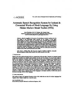
We show an overview of the speech production and recognition in figure 2.1. In this figure the connection between sending and receiving is described by the right and the left vertical arrows. Figure 2.1 is our simple modification of the speech chain given in [80]. The figure has two parts: • The upper part : Speech Generation • The lower part : Speech Recognition

2.2.1

Human Speech Generation

We describe the speech generation in brief only because it is not our central task. However, for certain aspects it is necessary for us to know something about the speech generation. Later on in the chapter we describe the vocal tract from an engineering point of view using speech acoustical information. Here we explain the influence of the vocal tract in the speech production and generation. This will clarify the motivation of the use of the vocal tract system in the speech research as a main organ in the practical speech production model for speech processing[30]. The process is described in steps:

10

Speech generation Articulatory motions Message formulation

Neuromuscular controls

Language code Discrete input

Vocal−tract system

Continuous input

Human being

Acoustic waveform

Message understand

Language translation

Discrete output

Neural transduction

Inner ear Basiler membrane motion

Continuous output Speech recognition

Figure 2.1: Speech Generation and Speech Recognition [80]

• The speech production process begins when the speaker formulates a message in the speaker’s mind and in the brain. That is what the speaker wants to say to the listener. • The next step is the language code. This converts the message into some text and phonetic symbols. These are the elements of a certain language governed by linguistics and phonetic rules. When the phonemes i.e. the acoustics units are in correct order, the speaker can pronounce an understandable word. For example, if the speaker wants to greet someone saying ”Good Morning” the speaker first needs to decide the language, e.g., if it is in German or in English. The result of the message formulation or the conversion of this message into a syntactic form is then sent to the neuromuscular controls. The smallest element in the speech is called a phoneme. The phonemes are given as sounds of a language produced by an individual speaker • Next the neuromuscular movement takes place to control the vocal apparatus, for example the vocal folds, or the nasal part or the lips that are needed to be moved to generate the message for instance here it is the greeting : ”Good Morning”. • When the loudness of the pitch is established, the vocal-tract system, for

11

instance the vocal-tract vibration, acts, the speaker can say ”Good Morning”. • The result of the whole process is a continuous time analog waveform at the lips, jaw, velum etc. In this way the speech waveform is produced. Here the generation process ends. We will not be concerned with the human speech generation and its automation. However, the generation process has to be understood to use it in the model that represent the spoken speech. The source excitation model discussed in chapter 6 is the most commonly used model to represent the speech generation process. The purpose of using this model is given in chapter 10 but some physical explanations of this model relating speech generation by the human being is given in section 2.4. The vibration rates of the vocal folds during the speech production while transmitting the process through the vocal-tract are different. Similarly, the speech waveform of formulating the message may change depending on the speaker.

2.2.2

Human Speech Recognition

For recognition we look at figure 2.1 to see what is intended. The message interpretation shown at the bottom right corner in figure 2.1 is the speech recognition or the speech perception. • The first step is an effective conversion of the acoustic waveform into a spectral representation. This takes place in the inner ear by the basilar membrane. This membrane acts as a non-uniform spectrum analyzer by spatially separating the spectral components of the incoming speech signals and analyzing them, for example using a non-uniform filter bank. • The next step is the neural transduction of the spectral features into a set of distinctive sound features. • These features are decoded and processed by the brain. This is described by linguistic rules. • Finally these features are converted to a set of phonemes, word sequences and sentences in order to understand or recognize the intended message (that was originally generated). This takes place in the brain and requires much human knowledge.

12

2.3

Speech Recognition by Machine

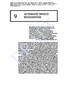
Here we give a pictorial motivation for the approach. Figure 2.2 shows how the speech recognition can be replaced by a machine. If we compare figure 2.1 and figure 2.2, we see in figure 2.2 that the tasks in the human ear and the brain is replaced by a machine. A basic understanding of the processes taking place in the human ear is useful for the speech recognition tasks. We see that these tasks are rather complex and require interdisciplinary knowledge, e.g. from the physics of sound transmissions, the physiology of the human auditory system, the human speech perception to begin with. We have given in chapter 11 a brief superficial introduction and outline of the study of the psychoacoustics that studies the human speech perception in order to capture an essence of human speech perception and perceptual speech recognition. These are introductions and outlines of the study of the psychoacoustics. We show how the psychoacoustics elements are quantized. Our main aim is to recognize noisy speech and this is discussed in next chapter 3. The ASR studies belong to an area of pattern recognition which Speech generation Articulatory motions Message formulation

Language code Discrete input

Vocal−tract system

Neuromuscular controls Continuous input

Human being

Acoustic waveform

Speech output(message)

Machine (e.g. computer) Speech recognition

Figure 2.2: Human Speech Generation and Machine for the Speech Recognition

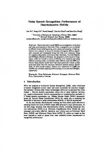
is to some degree a sub-area of machine learning. In the overview of an automatic speech recognition (ASR) system given in figure 2.3, we see the speech data as input are transformed into some trained set in order to apply some learning tool in the training phase. Then some test data are used by applying some search tool in the testing phase. Therefore the ASR system has two main phases: • Training Phase: Here the examples are given to machine learning.

13

• Testing Phase: Here some learning tool is employed and then classification of the examples in order to recognize the test data to find the overall the outcome as a result of the learning process takes place.

Training Phase Speech input

Feature extraction

Test speech

Training features

Feature extraction

Learning

Test features

Search

Result

Testing Phase Figure 2.3: Overview of ASR Process

There are different ways the generated speech can be represented in the machine. Two most common approaches are: • Parametric approach: Here some signal models are used to extract speech parameters. An example of the parametric approach is linear prediction analysis (LPC). They are individual for each speech act, unkown and have to be estimated. These parameters are the starting point for the speech recognition task. We followed this approach. This is discussed in chapters 6,7,8,9. • Non-parametric approach: FFT based analysis is an example of this approach. This is a commonly used tool to begin the speech recognition tasks. Examples of the non-parametric approach is MFCC discussed in chapter 12. The ASR architecture and structures are now briefly mentioned. An overview is shown in figure ??.

14

2.3.1

ASR Types

The speech recognition can be of different types. Thus the architecture and structure of the ASR can be varied. Below we provided a list of possible ASR types and their architecture [69], [80]. System Architecture This discusses acoustic and linguistic elements as e.g. phonemes, words, phrases and sentences. The structure of the ASR can be: • Continuous: Speech that is naturally spoken in a sentence. • Discrete: Discrete speech systems use one word at a time and it is useful for people having difficulties in forming complete phrases in one utterance. • Isolated: In isolated speech, single words are used and it is easier to recognize the speech. The type of the ASR can be : • Speaker Dependent : A speaker dependent system is intended for a use by a single speaker. In a speaker dependent system, necessary training data are : 100 different people saying the speech for instance 10 times separately and necessary testing data: 25 different individuals that are not in the list of the speakers in the training data collection saying the corresponding speech. • Speaker Independent: A speaker independent system is intended for use by any speaker; it is more difficult in the sense that it has more variations to be considered than the speaker dependent one. The speaker independent system involves a collection of thousands of data. The vocabulary size of the ASR can be: • Small Vocabulary: Tens of words for example a list of 10 to 100 vocabulary model. • Medium Vocabulary: Hundreds of words for example a list of 100-300 vocabulary model. • Large Vocabulary: Thousands of words for example a list of 1000- 10000 or more vocabulary. Some ASR applications and possible environment are :

15

• Examples are speech in a hospital or in a nursing home to monitor the patients, in an industry to command a machine, for dictating in law enforcement, in robotics to perform some intended tasks using some voice commands etc. • Environment: This can be noisy, moderate, mixed of noise and normal environment or quiet. Our DANSR specification is mentioned in chapter 3. The human speech generation process is captured for speech processing by the source excitation model.

2.4

Acoustics of Speech Production Model

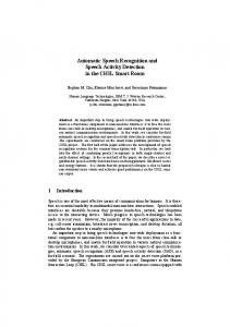
The acoustic phonetics studies the acoustic properties of the speech and how these are related to the human speech production. A standard computational speech production model is discussed in chapter 6 which makes use the study of the acoustics, phonetics, psychoacoustics and digital signal processing in order to model the speech process. The purpose of the computational speech production model is to manipulate the reality computationally and to estimate the constraints and the constants in the body. This correlates the physical process to a computational model for the processing.The constraints in this context are the natural regulations in generating the human speech and the constants are the weights or the speech parameters and the outputs. Next we present computational aspects about some basic components used in the model in an overview. They are concerned with both, the human body and the machine. The model is described in chapter 6. The vocal-tract is playing a vital role in the speech production discussed in chapter 6. In the next description we use partially some qualitative terms. The vocal-tract shown in figure 2.4 is considered a lossless acoustical tube. We see in the figure that the vocal-tract has different cross sectional areas denoted by A1 , A2 , · · · , A5 .

2.4.1

Resonant Frequency, Formant and Sampling Rate

The resonant frequency of the vocal tract tube is the peak frequency of the vocal tract tube. It happens when the particular frequency and the vocal tract

16

Glottis

A5

A4

A3

A2

A1 Lips

Figure 2.4: Sketch of the vocal-tract: Non-uniform cross-sectional area [118]

frequency coincide. The standing wave is the current wave in the vocal tract tube. These are intuitive simple definitions of the resonant frequency and standing or ongoing wave of the vocal tract. The details of this can be found in the area of the acoustics phonetics study which is not investigated further. Resonant Frequency and Formant A connection between the formant and vocal tract tube is shown in equation (2.2). The length l of the vocal tract tube is an odd multiple of λ which is the wavelength of the standing wave. λn indicates the wave length at n which is a positive integer number. (2n − 1)λn (2.1) l= 4 The length of an adult male vocal tract is approximately 17.7 cm long and the length of an adult female vocal tract is approximately 14.75 cm long [87]. The resonant frequencies fn for n = 1, 2, 3 · · · are shown in equation (2.2). The speed of the sound in the air denoted by c is assumed to be 35400cm/sec. The formants are defined by the spectral peak in the speech sound spectrum. They are determined by the resonance frequency. This means if the resonant frequency is 1500 Hz, then a formant is generated at 1500 Hz. fn =

(2n − 1)c c = λn 4l

(2.2)

Selection of Sampling Rate The relation between the sampling rate selection and the vocal tract architecture is shown in equation (2.4). The wave propagates in vocal tract cross-sections. In figure 2.4, the cross-sections of the vocal tract are denoted by A1 , A2 , · · · , An and n denotes a positive integer number. Suppose, the length of each tube is j, then the wave propagates in each

17

section is τ is computed by equation (2.3). τ=

j c

(2.3)

The discrete time system, the sampling rate of the vocal tract is 2τ seconds. The sampling rate fs is then can be expressed by equation (2.4) [30]. fs =

c 1 = 2τ 2j

(2.4)

The order of the model relating this to the physical vocal tract tube is discussed in chapter 8 in section 8.1.1.

2.4.2

Reflection Coefficients

As we mentioned earlier the vocal-tract is an acoustical tube which has several non-uniform sections. The waves that propagate from the tube are partially reflected and partially interrupted by the discontinuities of the junctions of the tubes. This is described by the reflection coefficients. The reflection coefficients reflects the vocal-tract structure, the shape of the vocal-tract and the speech transmission that is taking place in the acoustical vocal tube. The 0 value of the reflection coefficient means that all transmission in the vocal-tract tube are passed and 1 value of this reflection coefficients indicate that the transmissions are reflected [81], [87]. The reflection coefficients between two sections of the vocal tract can be shown by equation (2.5). The reflection coefficients are denoted by κ. κi is denotes the reflection coefficients for i = 1, 2, · · · , p. Ai and Ai+1 are the cross sections of the vocal tract tube where 1 ≤ i ≤ p. There are p many tube sections. A0 = ∞ is the area of the space beyond the lips and therefore it is a lossless transmission. κi =

Ai − Ai+1 Ai + Ai+1

where |κi | ≤ 1

(2.5)

The length of the vocal tract tube is determined by the sampling period and the speed of the sound as discussed in section 2.4.1. The reflections cause spectral shaping of the excitation which acts as a digital filter with the order of the system equal to the number of tube boundaries. The digital filter can be realized by a lattice structure. In this structure, reflection coefficients are used as weights. This is the background of the reflection coefficients and its use in the lattice structured

18

filter. This is briefly discussed in chapter 9 in section 9.3.1. The details of this can be found in [24].

2.5

Categories of Speech Excitation

From the speech acoustics point of view, an excitation type can be categorized by the following kinds of speech sounds [69]. • Voiced (Example: The letter /I/ sound in the utterance of ”six”) • Unvoiced (Example: The letter /s/ sound in ”six”) • Mixed (Example: The sound corresponding to the letter ”z” in the phrase ”three Zebras”) • Plosive (Example: A short region or silence, followed by a region of the voiced speech, the unvoiced speech, or both. A plosive example (silence + unvoiced) is the sound corresponding to /t/ in ”pat”. Another (silence + unvoiced) in the /b/ in ”boot” ) • Whisper is the pressure in the glottal area to utter any excitation types. We will see in chapter 6 how the above mentioned excitations types are simplified to the voiced and the unvoiced types and how these two types are modeled by only a single simple computational model to reflect the speech production process in reality.

19

Chapter 3 Noisy Speech Recognition Outline In this chapter we talk about noisy speech and its definition and handling this in our studies. We explain our aim, problems, challenges and difficulties relating these studies to the real world. We introduce the hybrid noise and their treatments. This incorporates different kinds of noises. Our solution approach takes care of this. This approach is mixed with a preview of literature about noisy speech evaluation and our own methodological approach. We introduce both active and passive noise solutions to this problem. For our approach an industrial environment is selected as an application area. What is new here to our perspective is that we provide a hybrid solution to our problem and the actions we take in order to arrive at the solution. In chapter 2, we provided a simple realization of speech generation, speech recognition by the human being and also a scenario of speech recognition by a machine. Here we talk about noisy speech recognition by a machine. The speech is in the first place not noisy by itself and it is noisy generally only after its generation by environmental factors. Next we first introduce to our noisy speech, hybrid noise, their impacts in section 3.1.

3.1

General Aspects

In general, an industrial environment is noisy. Here we are talking about a noisy industrial environment which is equipped with different types of machines, machinery handling and their operations such as manufacturing, assembling. The next figure 3.1 is not intended to be a definition. The corresponding definitions

20

are complex and come later when we discuss the technical aspects. 3.1 is rather thought of an illustration so that one can see in principle what we want to do. In figure, 3.1, we see that spoken commands are generated by a human being in a noisy industrial environment and given to a machine i.e. a computer for its recognition in the same environment. If we compare figure 2.2 given in chapter 2 and figure 3.1, we see the difference between the two figures. In figure 2.2, speech is generated in a clean environment but in figure 3.1 speech is generated in a noisy environment. In figure 3.1, the speech generated by a human being is delivered to a noisy environment. The speech is corrupted by the environmental noise. The Speech generation Articulatory motions Message formulation

Vocal−tract system

Neuromuscular controls

Language code Discrete input

Continuous input

Human being

Acoustic waveform

Speech output(message)

Machine (e.g. computer) Speech recognition

Noisy Environment

Figure 3.1: Noisy industrial environment: Speech Generation by a Human being and a Machine for the Speech Recognition

industrial noises are not all the same type. They have different intensity and extremity and we call this combination hybrid. Typically, we categorize them as strong, steady and mild. A reality is that we cannot process our data that we have collected from the noisy environment for its required enhancement and neither do we have an option to enhance the noisy observations by some standard noise reduction techniques. A main problem is that a ”common” approach or a ”standard” approach is not an appropriate solution approach to this hybrid noise. There is not yet any such solutions to the hybrid noise that could enhance the hybrid noisy speech for its recognition. Nevertheless, our scenario occurs quite often, see section 3.2. Though there is a huge amount of literature about noisy speech enhancement or noise reduction or removal [117], a majority of this [148] solves this problem by applying some standard noise solution approaches or standard digital filtering or some adaptive filtering such as Wiener filter, Kalman

21

filtering for white noise, or spectral subtraction, or sometimes a combination of one or more of them [86]. In fact, a hybrid noise solution has rarely been considered. The problem seems to be that it is not trivial to combine different techniques [46]. But the situation is that because of the different types of noise we need a hybrid treatment for them. For each type we apply a method based on the existing noise source. Each method will, however, not just remove or add something but will effect the whole signal. Here the main tasks for our noisy speech recognition problem are: • Removal or reduction of the noise that corrupts the speech. We use the removal or reduce the noise because both of these are done. The removal or reduce term is dependent on the type of the noise. • Recognition of the enhanced speech.

3.2

Scenario

In an industrial environment, a smooth communication is not possible and the necessity of removal or reduction of the noise in the desired speech becomes significant for an effective communication. There the noise is mixed and originating from different sources. These come for example from lifter systems and related machines or different types of conversations among people. We term strong noise as a sudden burst, press or dropping sound originating from various heavy material handling and falling down. The duration of this type of noise is very short. The time-varying steadyunsteady noise in our description is originating from varying electromechanical machines. We consider the remaining background noise as mild noise. A precise duration and formulation of the mixed noise from various sources is not possible in this hybrid noisy environment and precise mathematical definitions cannot be given. Hence we use qualitative arguments. Here we consider the noises that affect the commands at its duration which is in our case no longer than three seconds. It is not always possible to maintain an exact timing. The scenario of this studies is shown in figure 3.2 in an overview over the whole situation. Figure 3.2 is again only of an illustrative character, as common in artificial intelligence. There are elements of the speech, the noise and the system shown in a combined way to inform the user. We have a predefined command list. The environment is a closed world because the situation is precisely defined.

22

The task is to recognize the delivered speech in spite of the existing environment. Figure 3.2 shows the different inputs to the recognition system. The inputs can be desired spoken command, undesired different types of signals such as noise, the different types of environmental impacts. But the aim is that the recognition system recognizes the desired spoken command and omits the other undesired environmental influences. To fulfill the aim of the tasks, we have used different Industrial

Environment Noise 1 Noise 2 Noise 3

Human being

Noise n Conversations Desired Spoken Commands Environmental effects Environmental Impact

Speech Recognition System

Noise + Spoken commands

Recognized Commands

Figure 3.2: Hybrid Noise and Industrial Environment techniques and integrated them. However, the integration is somewhat different than in ordinary software systems. We have no modules where we just have to take care of input-output relations. Each technique concerns more or less with almost the whole system. We have to take care that certain properties of the system still hold and the system is interactive. Therefore the integration of the different techniques have to be embedded in such a way that an immediate interaction between the techniques applied to perform the tasks are possible.

3.2.1

Goals of DANSR

We focus on developing a small vocabulary speech recognition system. The small vocabulary speech is a set of small spoken words which we interpret as commands. This set of small words is spoken to a single microphone. The speech sound is a mixed tonal sound and it has a variety of variable patterns. The variability we

23

want to preserve is the speech acoustic information on the word level. For this we have a followed mainly the parametric modeling. We look first at the vocal tract configuration by a parametric model and use this model for noise reduction in order to obtain an enhanced speech, then we use the enhanced speech for a non-parametric spectral analysis and a perceptual speech feature extraction technique in order to obtain the features and finally we apply a model based pattern recognition technique for classifying the features and recognizing them. Thus the goal of the DANSR is : • An integrated approach to deal with the different types of noise simultaneously by the followings: 1. A suitable combination of mixed noise reduction approaches. 2. Extraction of perceptual speech features of the enhanced speech. 3. Pattern recognition techniques applying the Hidden Markov Model (HMM) which model is based on the Gaussian mixture model (GMM).

3.3

Noisy Speech and Difficulties

In our day to day life, we can not interpret or if we do not understand a speech of a speaker in case of an extreme strong noisy situation, we ask the speaker to repeat. The question is what not understanding means; there is no general definition. If the listener is a human then this is personal. A machine however needs a formal definition. We circumvent this problem by deleting the speech depending on the noise definition, see chapter 5. In an acoustic sense the sound or speech or noise is an atmospheric pressure waveform where its variation as it progresses and its differentiation is received subjectively. This means some sound or speech or noise may be perceived in different meanings from a person or may vary from theme to theme. For example loud music may be noisy to an individual or some conversation may be noisy to an individual but for others this may sound useful or not so influential. Regardless of an environmental influence, the aim is to recognize some predefined spoken command. We need to record as much variability as needed. We mention the necessary amount in chapter 4 in section 4.1. The speech sound is a stochastic process and variability is one of the major difficulties of this process. The success of an ASR system requires knowledge from multi-discipline areas such as electrical engineering that discusses signal processing, communication and

24

transmission, physics related to psychoacoustics, linguistics for example phonology, computer science as for instance pattern recognition, searching, logic etc. An individual can hardly attain all the required knowledge. Therefore, one has sometimes in practice a group research where the tasks can be sub-divided based on an individual’s expert knowledge. Sometimes the expense to continue this research is not available at the spot. Therefore, in many cases the success of the research may not be fully achievable. These are certainly some common challenges in this research. Below we talk about our ASR research problems and challenges.

3.3.1

Challenges

The speech signal has a complex pattern. It is mixed with different tones and varies with time. The speech signal has different frequencies and different intensities. The complex tonal sound has more processing complexities than a pure simple sinusoidal tonal sound. The variability of the speech signal makes the speech research complicated and challenging. A spoken command generated by a particular speaker several times is not the same. The utterances all have different frequencies and different intensities. Many factors are involved such as time, speaker, speaking style. Moreover, in our study, we have noisy speech to process for its recognition. The noise is originated from the background, from the environment. The environment is mixed with different kinds of noise. We have listed some common challenges of the speech recognition problem: • Variability of the speech due to a variety of speeches spoken by the same speaker. • Variability of the speech due to a variety of speakers speaking style. • Variability of the speech due to the speech linguistics formation. • A variety of environmental noise.

3.3.2

Difficulties

So far we mentioned the challenges; but what are the difficulties we encounter in the research problem? The human being itself has a difficulty to understand others in a noisy environment. Some additional difficulties we encounter are listed below: • Identifying the noise in the noisy environment.

25

• Modeling the hybrid noise. • Finding a proper solution to remove or reduce the noise that corrupts the spoken word. • Managing the collected noisy speech data for noise reduction and training. This means we cannot use the data directly for the noise reduction without preparing and pre-emphasizing the collected data. Also, only standard preemphasizing which is generally a first order high pass filter is not sufficient to prepare the noisy data for their further processing.

3.4

Noise Measurement and Distinction

The measurement of the noisy signal characteristics and the solution to the noisy signal problem can be passive or active or a combination of both. Here we will introduce the active and passive approaches and their application to our studies. • By ”active” we mean actions such as removal, filtering, Poisson modeling and matched filtering operations, and Kalman filtering. • By ”passive” we mean some standard measurements of the noisy speech or the noisy sounds. To distinguish noise, we first use the passive measurements. Then we apply the active approach. The active approaches are introduced here but the details of these are in chapters 4, 5,6,7,8,9,10. For the passive measurements, we first measure the loudness of the noisy speech using a standard A-weighting filter. We also calculate the energy of the noisy signals, compute the probability density function, use a box plot evaluation, and evaluate the noisy signals by computing the signal to noise ratio (SNR). We call these passive measurements because they do not make any changes and they do not improve the noisy speech by removing noises. Rather they give some information about our collected noisy speech.

3.4.1

Noise Measuring Filters and Evaluation

Since the situation is taking place in the bounded space i.e. in a factory which is a very spacious room in a building and we consider this as a ambient noise measurement. In such situation, sound levels are measured by sound level measurement

26

devices such as A, B, C, D, E-weighted filters. We choose the A-weighting filter among those device because the A-weighting filter accounts for the human hearing perception that is the human ear sensitivity [91]. This is a useful property for the speech recognition system. The A-weighting filter is also commonly used for the ambient environmental sound level measurement. The A-weighting filter measures the loudness of the average sound level over a period as a root mean squared power in dB. According to the statistical information and the sound level measurement, we have continuous, varying, intermittent, and impulse types of sound. We have a random noise level variation such as mixed noise levels varying from 60 dB to 115 dB. At 90 to 115 dB a communication is not even possible among the human beings. Such noisy environments damage our hearing capability. In such measurements, the range of 70 to 80 dB is in the mild-steady noise level, 80 to 89 dB is in the varying steady-unsteady and above 90 dB is strong noise level [23]. In figure 3.4, we see the sound levels of the noisy signals collected from hybrid noisy industrial environment. We have given the locations in chapter 4. The sound level is measured by A-weighting filter. 3.4.1.1

A-weighting Filter

The A-weighting filter has been used in the frequency domain of the signal. Here we explain how we have used this filter to evaluate the signal level of the noisy signal: First the spectrum of the noisy signal is computed using the discrete Fourier transform (DFT) and the A weighting filter is then applied to measure the signal power in dBA. The power spectrum of the N sampled signal s[n] where n = 0, 1, 2, · · · , N − 1 is computed by equation (3.1). S(k) =

N −1 X

|s[n]|e−

2πkn N

(3.1)

n=0

Equation (3.2) below shows a relation between the frequency response of the Aweighting filter denoted by αA (f ) and the linear frequency of the signal denoted by f . The measurements of A-weighting filter give us some intuitive idea about the signal and the sound level. From this we get an approximate idea about the enhanced signal level and use the enhanced signal for the feature extraction. Equation (3.2) is mainly collected from [26] and more information on this is in [135], [23], [91], [51], [49]. We use this formulation to generate the figures 3.4, 3.5, 3.6 using the implementation given in [49] and in [26]. The derivations and

27

formulations of the A-weighting filter is discussed in acoustic noise measurements, monitoring and control and some information about this studies can be found in [23], [91], [51]. The mathematical derivations and modeling of the weight filters are the results of many experiments to measure the loudness of the sound in sound pressure level (SPL) or in dBA [135]. We will not discuss the derivations of the filter here. We only use the filter to get an information about our noisy signals, their sound levels. We have modified the implementations given in [51] and [26] according to our own our measurements; the experimental results are shown in figures 3.4, 3.5 and 3.6. In figure 3.3, we see the noisy signal in time and frequency domain. This is included to get an outlook of the mixed noisy signal. a:Noisy Speech in time domain: Oeffne die Tuer

Signal Sample

1 0.5 0 −0.5 −1

0

0.1

0.2

4

0.4 0.5 0.6 Time (in second)

0.7

0.8

0.9

1

b: Noisy Speech Spectrum: Oeffne die Tuer

x 10 Frequency (Hz)

0.3

2

40

1.5

20

1

0

0.5 0

−20 0

0.5

1

1.5 Time (sec)

2

2.5

Figure 3.3: Hybrid noisy signal : Noisy speech signal in the time and in the frequency domain Figure 3.4 shows sound levels of our measurements using A-weighting filter. These are collected at different times from the mixed noisy environment. This figure implies the varying sound levels of the signals. (122002 )f 4 (f 2 + 20.5989972 )2 (f 2 + 122002 )((f 2 + 107.72 )0.5 )((f 2 + 737.92 )0.5 ) (3.2) If the frequency of signal spectrum S(k) measured at fk where k is the index of the frequency component then the A-weighting filter measurement for this αA (f ) =

28

b:Steady unsteady noisy signal Signal Level (dBA)

Signal Level (dBA)

a:Mild noisy signal level 90 80 70

0.5

1 1.5 Time (second) c:Strong noisy signal

2

70

2.5

0

95

Signal Level (dBA)

Signal Level (dBA)

80

60

60

90 85 80 75 1 1.5 Time (second) e:Typical quiet signal

80 60 40

0.5

1 1.5 Time (seond)

2

2.5

0.5

1 1.5 2 Time (second) d:Mixed noisy signal

0.5

1 1.5 2 Time (second) f:Typical noisy signal

2.5

74 72 70 68

2

Signal Level (dBA)

0.5

Signal Level (dBA)

90

2.5

90 85 80 75 70 0.5

1 1.5 Time (second)

2

2.5

Figure 3.4: Hybrid noisy sound level measurements by an A-weighting filter

29

frequency at specific index k is obtained by equation (3.3) for fk = k∆f = fNs = 1 . fs is the sampling frequency, N is the length of the interval. Here we have NT chosen N = 256. The DFT is computed at each N interval. T is the sampling period T = f1s . The frequency resolution denoted by ∆f is N1T . The A-weighted signal level measurement denoted by SA (k) is computed by the multiplication of the A-weighting filter frequency response and the noisy signal spectrum S(k) in equation (3.3). SA (k) = αA (fk )S(k) (3.3) Then the signal energy ζ shown in equation (3.4) is computed by squaring the spectrum of SA (k) for 0 to N2 − 1 because of the symmetry property of the Fourier transform. N −1 2 X ζ=| SA [k]|2 (3.4) k=0

Next the signal level in dBA is computed by equation (3.5) where ζref is reference pressure and its value is 0.000204 dynes/cm2 . Signal level in dBA = 10 log10

ζ ζref

= 10 log10 ζ − 10 log10 ζref

(3.5)

In equation (3.5), ζref is a constant which is replaced by a calibration constant in its real application. Signal level in dBA = 10 log10 ζ + C

(3.6)

In our measurements, we use a calibration constant of 55 dBA because in a noisy environment a human being can perceive sounds in the range of 50 to 90 dBA [91]. In figure 3.5, the signal level is computed on the frame (defined in chapter 12) of the signal using an A-weighting filter. In this 3-D figure, we see the sound level, time and frequency information of the hybrid noisy signal.

3.4.2

Box Plot Evaluation

The box plot shows the distribution of data in general. This represents the data using their lowest value, highest value, median value and the size of the first and the third quartile. The median is counted by equation (3.7) and is denoted by d(m) where m denotes the median and n is the number of data points in the

30

Sound label measured in signal frames

0

Sound Level (dBA)

−20 −40 −60 −80 −100 −120 −140 30 100

20

80 60

10

40 20

Frame number

0

0

Frequency band

Figure 3.5: Noise level and noisy signal energy in signal frames

31

observation.

n+1 (3.7) 2 The depth dql of the quartile is shown in equation (3.8). There n is the number of data points in the observation, i takes the value based on the quartile depth i.e. i takes the value of l. In equation (3.8), dq1 denotes the first quartile. i can be 2, 3, or 4 which indicates the corresponding quartile. d(m) =

dql =

in + 2 4

(3.8)

In figure 3.6, we see a number of noisy signals denoted by dat1, dat2, dat3, · · · , dat10 on the boxplot. We see there the noisy signals and their samples values and signal level in a box plot.

b1: Boxplot of some Collected Speech Signal

Amplitude

1 0.5 0 −0.5 −1 dat1

dat2

dat3

dat4

dat5

dat6

dat7

dat8

dat9

dat10

dat8

dat9

dat10

Power level in dBA

b2: Estimated power level of the signals 70 60 50 40 30 20 dat1

dat2

dat3

dat4

dat5

dat6

dat7

Figure 3.6: Hybrid Noisy Signals : Sound level in Box plot The part between the lowest adjacent limit and the bottom of the box represents one-fourth of the data. One-fourth of the data falls between the bottom of the box and the median and another one-fourth between the median and the top of the box. The part between the top of the box and the upper adjacent

32

limit represents the final one-fourth of the data observations. This opens up the pattern for the data and their variations [138].

3.4.3

Signal Energy and Kernel Density Estimation

In figure 3.7 we see the energy information of the noisy signals in the signal frame (defined in chapters 8, 12) and in b, we see the probability distribution of the samples values computed by probability density function (pdf) of the noisy sigP −1 2 nals. The energy of the signal is computed in figure 3.7 by N n=0 s[n] where n is an integer i.e. Z and sn is a signal of finite length N . The probability density function of the random variable X is calculated using the kernel probability density estimation (k-pdf). We assume n independent measurements such as x1 , x − 2, · · · , xn from the random variable X is considered. The kernel density function approximates the probability density function of p() of the random variable X. The computation is available in matlab. For this we have used the matlab ”kdf” function. The calculation is followed by the formulation given in equation (3.9). In this equation, ph (x) is the pdf as a function of x. h is a normalization factor; h > 0 but less than 1 and dependent on the available information of x. Here x is independent and identically distributed (iid). Here K() denotes kernel function, x is any value and xi is a sample of the x [18], [137]. n

ph (x) =

3.4.4

1 X x − xi ) K( nh i=1 h

(3.9)

Signal to Noise Ratio (SNR)

We judge the speech intelligibility by the signal to noise ratio (SNR). The speech intelligibility says if the speech is audible or not. The signal strength and noise strength are primarily measured by the signal to noise ratio (SNR) in dB. This gives a relative performance of the signal with respect to noise. If the signal strength is higher than the noise strength, the ratio is positive. If the noise strength is higher than the signal strength, then the SNR is negative. The SNR is computed by equation (3.10). There the SNR is denoted by κm , Ps is the power of the signal and Pn is the power of the noise. The whole signal is divided into M segments such that m = 1, 2, · · · , M . There N is the number of samples in each m. ym [n] is noisy speech, bm [n] is the noise collected from the

33

a: Energy of the hybrid noisy signals

b:pdf of hybrid noisy signals

1

14 s1 s2 s3

0.9

s1 s2 s3

12

0.8 10

0.6

8 pdf

Signal Energy

0.7

0.5

6

0.4 0.3

4

0.2 2 0.1 0

0

2

4 Time in second

6

0 −2

8 4

x 10

−1

0 Signal in time

1

2

Figure 3.7: Hybrid noisy signal : Signal energy in signal frames and pdf of noisy signal environment without speaking commands to the microphone. κm = 10 log10

3.5

Ps = 10 log10 Pn

PN −1 2 1 n=0 ym [n] N P N −1 1 2 n=0 (bm [n]) N

(3.10)

Overview of DANSR

The different kinds of noises characterize the situation as hybrid. As said, we need a hybrid solution consisting of different elements. A major problem is the integration because these elements influence each other and cannot be combined in an arbitrary order. Figure 3.8 shows the DANSR system. This gives a rough overview. Details of the approaches and their motivations are discussed in the subsequent chapters in the thesis. In the figure we see, first we focus on reducing the noise, then we apply the perceptual feature extraction consisting of spectral shaping, spectral analysis and perceptional feature transformation, and finally the GMM model, evaluation, searching and learning in the classification and recognition stage to obtain the most likely result. Details of the approaches represented in figure 3.8

34

are in the subsequent chapters. Speech Generation by Human being Message formulation

Neuromascular control

Language code

Vocal tract system

Acoustic waveform

Human being

Industrial Speech output(message)

Machine (e.g. Computer)

Environmental Hybrid Noisy

Recogniton result

Spoken Command

Learning (Baum−Welch) Search space (Viterbi)

Data preparation

Spectral shaping

Features

Mild noisy speech Spectral analysis

Perceptual Feature transformation

M−band Kalman filter

Yes Varying unsteady−steady noise solution

Speech audible Yes/No ?

PLTT Feature extraction

No Repeat

Classification and Recognition (HMM)

Strong noise solution Outlier removal Feedback

Evalutation (Forward) Acoustic model (GMM)

noise

Speech Recognition by Machine Dynamic Automatic Noisy Speech Recognition System (DANSR)

Figure 3.8: Hybrid Noisy Speech Recognition: Framework of DANSR

Above we have introduced active and passive processes. Now we extend these notions to tasks and they will be discussed now. Passive Tasks Data collection and their proper management, noisy signal evaluation. Active Tasks Pre-emphasizing the collected data, active noise reduction approaches, perceptual feature extraction and classification and recognition of the features.

3.5.1

DANSR’s Hybrid Noise Treatments

The noise treatments of the DANSR are introduced next.

35

3.5.1.1

Noisy Speech Pre-emphasizing

According to our plan to maintain a precise 3 second speaking time for the data collection was sometimes difficult. Despite the noise, the speaker’s speaking style, accent and non-speech or silence in between added more redundancy in the data. Therefore we smoothened the data prior to its processing. We termed this preemphasizing. This is discussed in chapter 4. We collected spoken commands. These collected spoken commands are our data. We present a short overview over the considered noise types that will be detailed in the following chapters. 3.5.1.2

Strong Noise

As mentioned, this noise occurs rarely, randomly for a short time period. We call a very short pulse with very high amplitude strong noise. We are not accurate about its occurrence but it happen stochastically and we are not certain about its effect on the spoken commands. For the strong noise there are no absolute numbers given. Our sizes have a qualitative character. They are defined in relation to the average noise. For this purpose we choose a threshold. A noise signal is considered as strong if its amplitude exceeds the threshold. The strong noise is handled first by detecting it as an outlier. This is an abnormal quantity in an observation. The identification of outliers is a standard difficult problem in data analysis. In chapter 5 we will discuss strong noise in detail. Here we just mention that it is modeled by a Poisson statistics. We see in figure 3.9 a signal that is modeled by Poisson process. This says the Poisson process xt generates the strong noise 5 times in a time period of duration t = 2. λ is the occurrence of the event which is the strong noise and t is the time interval. 3.5.1.3

Mild Noise

The mild noise is modeled as white noise. This noise is characterized by a Gaussian process. This is commonly known as white Gaussian noise (WGN). There the mean denoted by µ is zero and variance denoted by σ is 1. For instance, take a Gaussian process x for time instants n and n = 0, 1, 2, · · · , N − 1. Then x[n] and x[n+1] are independent and uncorrelated. This indicates E{x[n+l]x[n+m]} is zero for l 6= m and l, m ∈ Z. The mild noise is shown in figure 3.10 where we see the time domain plot of WGN, autocorrelation of two WGN sequence is 1. The variance of white noise is 1 and mean 0. The frequency information of WGN is also shown. These plots are generated using matlab functions rand, xcorr and

36

Distribution of xt for Poisson(λ = 5) 0.25

0.2

P(xt=2)

0.15

0.1

0.05

0

0

1

2

3

4

5 Time t

6

7

8

9

10

Figure 3.9: Strong noise modeled by Poisson process fft. The rand generates uniformly distributed random sequences, fft gives the frequency information of of the WGN and xcorr computes the auto-correlation between the two random squence at time n + l and n + m. This Gaussian process is also known as normal standard distribution process. The probability density function (pdf) of this noise is shown in equation (3.11). p(x) = √

1

(x − µ)2 1 x2 √ ) = ) exp(− 2σ 2 2 2π

(3.11) 2πσ 2 The model of mild noise is characterized by white Gaussian process is used in eq (3.12). σ 2 = E{[x2 [n]]} (3.12) 3.5.1.4

exp(−

Steady-unsteady Time Varying Noise

This noise comes from a running machine. This is characterized as a Gaussian process but its mean µ is not zero and the variance σ may not be always 1 as it is the case for the white Gaussian noise. If x is a Gaussian process for time instants n and n = 0, 1, 2, · · · , N − 1, and its mean is µ and variance σ, then the pdf of the noise is characterized by equation (3.13) where p(x) is the pdf of x. The colored noise modeled by the Gaussian process is pictured here in figure 3.11

37

a: White Gaussian Noise (WGN) 4

x(n)

2 0 −2

Autocorrelation of WGN

−4

0

0.2

0.4

0.6

0.8 1 1.2 1.4 Time (s) b: Autocorrelation of WGN noise

1.6

1.8

2

−0.5 −50

−40

−30

−20

−10 0 10 20 Lag [samples] c: Frequency information of WGN

30

40

50

50

100

150

400

450

500

1 0.5 0

0.2

|X(k)|

0.15 0.1 0.05 0

0

200 250 300 Frequency (Hz)

350

Figure 3.10: Mild noise modeled by white Gaussian noise (WGN) where we see the random Gaussian noise, its auto-correlation and the frequency information computed by matlab fft and corr functions. p(x) = √

1 2πσ 2

exp(−

(x − µ)2 ) 2σ 2

(3.13)

The noise model shown in equation (3.14) is an AR model but its parameters are obtained by the linear prediction namely the Yule-Walker approach. In equation (3.14), the noise d[n] is a linear combination of past i many β coefficients and a disturbance w[n]. This is assumed to be a white noise and it is weighted by gb . d[n] =

q X

βi d[n − i] + gb w[n]

(3.14)

i=1

For treating this noise, the signal is first divided into sub-bands using a cosine modulated quadrature mirror filter bank (QMF) and then the noise is minimized from each sub-band by a spectral minimization technique. Afterwards the signal is enhanced in each band by Kalman filter. In this noise reduction, noise is varying in each sub-band. The solution of this is discussed in details in chapter

38

a: Colored Noise

Amplitude

1 0.5 0 −0.5

Autocorrelation of Colored Noise

−1

0

0.2

0.4

0.6

0.8 1 1.2 1.4 Time (s) b: Autocorrelation of Colored Noise

1.6

1.8

2

−0.5 −50

−40

−30

−20

−10 0 10 20 Lag [samples] c: Frequency information of Colored Noise

30

40

50

50

100

150

400

450

500

1 0.5 0

0.2 |X(k)|

0.15 0.1 0.05 0

0

200 250 300 Frequency (Hz)

350

Figure 3.11: Time varying steady-unsteady noise modeled by Gaussian process 10. Next we present the framework of our DANSR approach.

3.5.2

Framework of DANSR

The architecture of a typical ASR was introduced first in chapter 2 in section 2.3.1. The DANSR is a small vocabulary speech recognition system. The DANSR uses basically the HMM. The frame work has the equation written below as a central element. This is repeated here but it is discussed in detail in chapter 14. In the equation p(o|q, λ) is called an acoustic model where the likelihood of the features given the model λ has to be obtained. o is the feature vectors, q is the sequence of states. The equation is discussed in chapter 14 in section 14.1. p(q|o, λ) = arg max q

p(o|q, λ)p(q, λ) = arg max p(o|q, λ)p(q, λ) q p(o)

If we look at figure 3.8, then we see that the main key tasks of the DANSR are: • Data collection • Noise reduction or removal

39

• Feature extraction • Classification and recognition These tasks give a guide for the dissertation.

40

Chapter 4 Pre-emphasizing of DANSR Outline of the Chapter In this chapter we describe our data collection, their preparation and their pre-emphasizing. We realize our data preparation and data pre-emphasizing by pre-filtering. This reduces the redundancy and smoothens the data in two steps: i) Redundancy removal, and ii) Pre-emphasizing by preemphasis filter. In the reduction step, it removes silence and then it uses the prefiltering to smoothen the data. The reduction step makes the data size smaller. How this is performed is explained in this chapter.

4.1

Data Collection

The speech is a random process. The statistical properties such as mean, variance, correlation, probability density function (pdf), power spectral density are used primarily to describe the signals. For the processing and recognition we need a huge number of data in order to capture certain patterns and the statistics of the data. We have a predefined list with small spoken commands. The list has 20 small German spoken commands. We collected data according to our predefined list (see Appendix). We have used the digital recorder Zoom 4 Samsung Handy Recorder to collect our data and noise taking place in the industrial environment. Our selected data type is in ’Wave’ format and we have used single channel only. We collected data using 48000 Hz sampling rate at 16 bits per sample. We positioned the recorder about 3 to 5 meters from the speaker for our data collection. We did this to avoid flappy sound or any clicking sounds generated in the mouth. The length of the data is 3 sec for each command. Therefore sometimes the speaking time

41

limit was exceeded. Furthermore in the noisy stage, the speaker’s speaking style, accent and non-speech or silence in between added additional redundancy in the data.

4.1.1

Location and Data Collection

The data are collected from the mechanical assembling and manufacturing laboratory of the university of Kaiserslautern, the environmental maintenance company Zoeller-Kipper Gmbh located in Mainz and the assembling and manufacturing company MM Packaging located in Kaiserslautern. In figure 4.1, we see the data we collected from the hybrid noisy environment. We collected the data from 4

a:Oeffne die Tuer

x 10 Frequency (Hz)

Amplitude

1 0.5 0 −0.5 −1

0

0.5

1 Time(sec) b:Oeffne die Tuer

1.5 1 0.5 0

1.5

Frequency (Hz)

Amplitudes

50

0 −0.5 0

2 1.5 1

0

0.5 1 Time(sec) c:Oeffne die Tuer Frequency (Hz)

−0.5 1 Time(sec)

1.5

0

0.5 1 Time (sec) 4

0

0.5

−50

x 10

0.5

0

0

0.5

1 Amplitudes

0.5 1 1.5 Time (sec) 4

0.5

−1

0 x 10

1

−1

40 20 0 −20 −40 −60 −80

2

1.5

0

1 −50

0.5 0

2

50

2

0

0.5 1 1.5 Time (sec)

Figure 4.1: Data at first look at 48 kHz sampling rate German speaking people. Each command is collected 100 times for training and 25 times for testing. The speaker is selected randomly from the environment. In

42

some cases the same speaker repeated the commands several times for the training. On the other hand, for the testing the speaker is not necessarily always the same. For our data processing, we are mainly concerned about the noise in the range of 200 to 5000 Hz for certainty at a speech bandwidth 200 Hz to 3500 Hz. In an industrial environment, a communication can take place if the background sound level is 70 dBA [23]. The noise we encounter has different extremity. This ranges from 50 dB to 110 dB. Reducing the redundancy and then using a pre-emphasis filter to smooth and emphasize the signal is so far new in this area. We applied this at the very first step to prepare our data for their further processing. Our focus for the speech enhancement is 70 dBA sound level. We then use this speech for the speech pattern recognition processing. We are concerned about building an acoustic model. To build such a model related to a speaker dependent system, a recognizer needs several hundreds of data. On the contrary, for a speaker independent system, a recognizer needs several thousands of data [120]. A collection of several thousands of data is not possible at the current scope of our research studies, therefore we consider a system that will be speaker dependent. In figure 4.2, one sees how the same speech is different for the same speaker. This variability is one of the main reasons among others that makes this research very challenging. We reduced some redundancies by applying an application dependent threshold. In order to prepare the data for the processing, we first decimated the data to a 16 kHz sampling rate, then we reduced non-speech pause, silence in the redundancy removal stage. How these are done is discussed below.

4.2

Data Preparation

The redundancy of the collected data is handled in removing and pre-emphasizing by the following steps: • Decimation: This is a process that reduces the sampling rate by a factor. This process has two steps: i) Antialiasing filtering and ii) Down-sampling. The anti-aliasing filtering is used to avoid aliasing. For the anti-alising filter, we have used a low pass filter. This is designed using the windowing method. For the windowing, we used the Kaiser window function because of its controlling parameters. The Kaiser window has a shape controlling

43

4

a:Oeffne die Tuer

x 10

50 Frequency (Hz)

Sample Amplitude

1 0.5 0 −0.5

2

1

0

0.5

1

1.5 2 Time(sec) b:Oeffne die Tuer

2.5

0

3

2

Frequency (Hz)

50

0 −0.5 0

1

2 3 Time(sec) c:Oeffne die Tuer

4

2

1

−50

0.5 0

5

0

1.5

−100 0

1

2 3 Time (sec)

4

4

x 10

1 Frequency (Hz)

50

0.5 0 −0.5 −1

1 Time (sec) 4

0.5

−1

0 x 10

1 Amplitudes

−50

0.5 −100

−1

Amplitudes

0

1.5

0

0.5

1

1.5 Time(sec)

2

2.5

2

−50

1 0.5 0

3

0

1.5

−100 0

1 2 Time (sec)

Figure 4.2: Variability of the same word spoken by the same speaker in the time and frequency domain at 48 kHz sampling rate in a relatively quiet residential environment

44

Speech Input s‘[n]

Aliasing free Speech Anti−aliasing s_[n] Downsampling filter factor (D) (Low−pass filter)

Down−sampled Speech s[n]

Aliasing free Down−sampler

Figure 4.3: Decimator: Data is downsampled from 48 kHz sampling rate to 16kHz sampling rate parameter such as width of the main lobe and side lobe. Then we have used down-sampling by the factor 3. Here the sampling rate is reduced from 48 kHz to 16 kHz. • Redundancy removal: This has several sub steps in order to remove the pauses in the speech or silence or non-speech sound of the speech signal. The sub-steps are: i) Compute the signal envelop by using the Hilbert transform and ii) Select the threshold. This reduces the redundancy and shortens the signal. It has a computational benefit due to less samples in the signal processing. Next the decimation process is described.

4.2.1

Decimation

For the decimation, we first down sample from 48,000 to 16,000 Hz. This has a computational benefit and is explained below. For this we do not loose information because the speech signal is band-limited 200 to 3500 Hz. The human audible signal frequency lies between 20 Hz to 20 kHz. Yet most of the speech energy lies under 7 kHz [19]. Figure 4.3 shows the decimation process which has an antialiasing filter before down-sampling the signal. The antialiasing filter is a 64 length finite impulse response (FIR) low pass filter based on the Kaiser window, the cutoff frequency is 5 kHz,the Nyquist sampling rate is 8 kHz. The down-sampling factor is 3. In matlab, the resample function also does this down-sampling but we used the Kaiser window based low pass FIR filter for the decimation. Computational Benefit Here we explain how the decimation is computationally beneficiary. If the speech recording time has a maximum of 3 sec, and if the

45

speech signal is sampled at 48 kHz at 16 bits per sample (bps) i.e. 16 bps, then the storage space for the sampled speech is 3  16  48 = 2304 kilo bits per sample (kbps) or 31648 = 288.5 kilo byte per sample or 31648 = 0.282 mega byte per 8 81024 sample (mbps).  denotes the muliplication. This is doubled for the stereo typed two channels recorded samples. Therefore we selected the single channel stereo typed data where both channels record the similar information. If the sampling rate is 16 kHz at 16 bits per sample, then the required space for the sample is 3  16  16 = 768 kbps. So the down sampling in our scenario will save a huge computational cost and a lot of processing time.

4.2.2

Envelope Detection

The envelop of a signal is a boundary within which the signal is contained. The envelop of a signal is also an estimate of the signal level. The pause or any clicking distortion or the silence in the speech signal is detected by the envelop of the speech segment [108]. One way of doing this is computing the envelop of the signal by the Hilbert transform of the signal. We have not investigated the Hilbert transform in details. We reviewed this only in order to compute the signal envelop. The basic goal of the Hilbert transform in the time domain signal is to get another time domain signal. The Hilbert transform shifts the frequency components of the signal by −90 degree but it does not change the amplitude. The Hilbert transform acts as a differentiator to a constant signal. This means if the signal has any constant component, the Hilbert transformation of the signal cancels this. This is equivalent to getting the zero mean of the signal. The speech signal is processed under the assumption that it is an ergodic process. In this process, the time average of the signal is equivalent to the ensemble average of the signal. The importance of this is that the time average of the signal can be computed easily but the ensemble average can not. This time average processing and more about the speech ergodic process we will see in chapter 7 and 8. In order to compute the envelope of the signal, we first take the Hilbert transform of the signal. The envelope signal has a frequency that is much lower than the measured signal. The problem is that the envelope makes the signal rough [106]. On the other hand the pre-emphasis filter increases the frequencies from low to high smoothly. The computation of the envelop using the Hilbert transform also maintains a representation of the signal. The envelop of the signal using the Hilbert transform

46

sets a qualitative boundary around the silence. We have used this computation to obtain the envelop of the signal. Then we have selected the threshold. We exclude all the data that fall below the threshold and remove pause, silence typed redundant data. The advantage of the smoothing is that we get less computational costs due to reduced amount of data because of the non-speech signal removal. 4.2.2.1

Formulations

Below we mention the relevant formulations for these computations. For this we follow the formulations mentioned in [106]. The Hilbert transform of the signal s[n] is denoted by sH [n]. How we computed 1 this is given in equation (4.1). This says the convolution of the signal s[n] with πn gives the Hilbert transform of s[n] denoted by sH [n]. ⊗ denotes the convolution operation. 1 ⊗ s[n] (4.1) sH [n] = πn In equation (4.2), we see how the envelop is computed using the real valued signal s[n] and the Hilbert transformed signal sH [n]. p | sA [n] |= {s[n]2 + sH [n]2 } (4.2) In figure 4.4, in a we see the spectrum of oeffne die Tuer computed by FFT where frequency along the x-axis and amplitude of the frequency information of the signal along the y-axis. In the same figure in b, we see the spectral envelop of the oeffne die T¨ ur. The spectral envelop shows the signal amplitudes versus frequency in the plot. In b, we see the FFT spectrum of the envelop computed by Hilbert transform. For implementation, we used the existing matlab function hilbert to compute the Hilbert transformation.

4.2.3

Adaptive Threshold Selection

The silence intervals from the speech are removed using a threshold. One commonly takes for the threshold one fourth of a median of the envelop for removing speech silence or pause or clicking sounds from spoken speech. There is again no precise reason for doing so. Then the speech samples with amplitudes below the threshold are detected similar to literature [4]. This literature detected these samples and deleted the non-speech sound from the speech. Thus the removal of the pauses shortened the time and thus the length of the signal.

47

a: FFT of Oeffne die Tuer

b: Envelope Detection of Oeffne die Tuer by Hilbert Transform

0.4

0.18

0.35

0.16 0.14

0.3

0.12 Amplitude

Amplitude

0.25 0.2

0.1 0.08

0.15 0.06 0.1

0.04

0.05 0

0.02

0

500

1000

1500 Frequency (Hz)

2000

2500

0

3000

0

500

1000

1500 Frequency (Hz)

2000

2500

3000

Figure 4.4: Spectrum of hybrid noisy speech and spectrum of envelop computed by Hilbert transform In figure 4.5 we can see how the redundancy of the data is removed by applying decimation, envelop detection and then the threshold selection. The recorded samples in a are reduced from 85056 times 2 to 26287 times 1, in b 61697 times 2 to 17908, in c 84096 times 2 to 25142 times 1. These data are easier to process than the originally recorded data. 2 means two channels. We have used only one channel but the information on the two channels are about the same. The two channels record data in two directions such as left and right. One channel can be selected only for the right or for the left direction. Alternative Recommendation An alternative to this redundancy removal approach is to apply Savitzky Golay filters to the raw signal envelope before computing the phase and its derivative [108]. But we have not yet investigated this approach.

4.3

Pre-emphasizing and Pre-emphasis Filter

The purpose of the pre-emphasis filtering and its effect is discussed here. In the speech processing literature equation (4.3) is seen as pre-emphasizing the signal and the filter in equation (4.3) is known as pre-emphasis filter [80]. A common way of seeing the application of a pre-emphasis filter is to emphasize the frequency component by considering both the low and high frequency components of the signal. The formants lie in the frequency range from 200 to 3500 Hz. The speech signal is a relatively low frequency signal.

48

a : Oeffne die Tuer 8000 Frequency (Hz)

Amplitude

1 0.5 0 −0.5 −1

0

0.1

0.2 0.3 0.4 Time(sec) b : Oeffne die Tuer

Frequency (Hz)

Amplitude

0 −0.5 −1

0

−60 0

0.5 1 Time (sec)

1.5

8000

40

6000

20 0

4000

−20

2000

−40 −60

0.1

0.2 0.3 Time(sec) c : Oeffne die Tuer

0

0.5 Time (sec)

1

8000 Frequency (Hz)

Amplitude

−40

0

1 0.5 0 −0.5 −1

−20

2000

0.5

0.5

0

4000

0

1

20

6000

0

0.1

0.2 0.3 Time(sec)

0.4

40 20 0 −20 −40 −60 −80

6000 4000 2000 0

0.5

0

0.5 1 Time (sec)

1.5

Figure 4.5: Redundancy removed signal and sampling rate is 16 kHz: Time domain plot and spectrogram

49

0

The redundancy removed signal denoted by s [n] is then used to pre-emphasize the high frequency of the speech signal prior to its analysis. The pre-emphasis follows 6 dB per octave rate. This means if the frequency is doubled, then the amplitude increases by 6 dB. The speech sound has normally higher amplitudes in the low frequencies than in the high frequencies. The pre-emphasize filter is identical to the filter that is used to model the lip radiation filter discussed in chapter 6. The pre-emphasis filter cancels the effect of the glottis. The system difference equation is presented in equation (4.3). The system is shown in figure 4.6. We see the result of the pre-emphasis filter is the emphasized signal s[n] if the input signal is s0 [n]. This pre-emphasis filter reduces

s ’[n]

s [n] + a em

z −1

’ s[n−1]

Figure 4.6: Pre-emphasis filter

the effect of 6dB/octave loss occurring by the glottal source and lip-radiation. s[n] = s0 [n] − aem s0 [n − 1]

(4.3)

Equation (4.3) can be rewritten in equation (4.4) in the z-domain by replacing s0 [n − 1] = S 0 (z)z −1 . S(z) = S 0 (z)(1 − az −1 ) = S 0 (z)Hem (z)

(4.4)

The transfer function of the pre-emphasize filter shown in equation (4.5) is just a high pass filter where we have approximately aem close to 1, for example 0.97. The determination of the coefficient aem is an empirical adjustment. This is again not precisely defined. The z-transform of equation (4.3) results in equation (4.5) . Hem (z) = 1 − aem z −1

50

(4.5)

In this equation, if aem > 0, the pre-filter acts as a low-pass filter and if aem > 0, the filter is a high-pass filter. The frequency response of this filter increases slowly from low to high, therefore it sets up a balance between the high and low pass frequencies [114]. The parameter aem controls the slope of the curve [147]. Therefore, this pre-filter may be called a pre-emphasis filter. In figure 4.7, we see the amplitude and phase response of the pre-filter for aem = 0.97. This response also shows that it is a high pass filter. a: Amplitude Response

b: Phase Response

10

80

5

70

0

60 Phase(Degree)

Magnitude(dB)

−5 −10 −15

50 40 30

−20 20

−25

10

−30 −35

0

2000

4000 6000 Frequency (Hz)

0

8000

0

2000

4000 6000 Frequency (Hz)

8000

Figure 4.7: Amplitude and phase response of the pre-emphasis filter

In figure 4.8, a shows the noisy signal which is pre-filtered as it is shown in b. In the same figure c shows the spectrum of the noisy speech and d is the spectrum of the pre-filtered speech. In figure 4.9, aem is the redundancy removed speech signal which is pre-filtered in b. In the same figure c shows the spectrum of the redundancy removed signal and d shows the spectrum of the redundancy removed pre-filtered speech. In both figures 4.8 and 4.9, we see the frequency is flattened by the employment of the pre-filter. This amplifies the high frequency components and attenuates the low frequency components. In figure ??, the industrial noisy speech and its pre-emphasized signal is shown. We can see in the figure a substantial amount of non-speech typed samples are removed. For this visualization , we have used Praat software [102].

51

a: Noisy Speech: Oeffne die Tuer

b: Pre−filtered noisy Speech 0.2

0.5

Pre−filtered S[n]

Speech Sample S[n]

1

0 −0.5

0.1 0 −0.1 −0.2 −0.3

−1

0

0.2

0.4 0.6 0.8 Sample Number (n)

−0.4

1

Amplitude of Spectrum

Amplitude of Spectrum

2

0.04 0.03 0.02 0.01 0

0

2000 4000 6000 Frequency (Hz)

0.2

d:Prefiltered noisy Spectrum

0

2000 4000 6000 Frequency (Hz)

1

1.5 1 0.5 0

8000

0.4 0.6 0.8 Sample Number (n)

x 10

−3

c: Noisy Spectrum: Oeffne die Tuer 0.06 0.05

0

8000

Figure 4.8: The effect of pre-emphasis filter on the speech signal: Noisy signal

52

a: Redundancy removed Speech

b: Pre−filtered Redundancy Removed Speech 1

0.5

Pre−filtered S[n]

Speech Sample S[n]

1

0

−0.5

−1

0

0.5 Sample Number (n)

0.5

0

−0.5

−1

1

c: Speech Spectrum 4

0.05

Amplitude of Spectrum

Amplitude of Spectrum

0.06

0.04 0.03 0.02 0.01 0

0

2000 4000 6000 Frequency (Hz)

0.5 Sample Number (n)

1

d:Prefiltered emphasized Spectrum −3 x 10

3

2

1

0

8000

0

0

2000 4000 6000 Frequency (Hz)

8000

Figure 4.9: The effect of pre-emphasis filter on the speech signal: Redundancy removed signal • Industrial hybrid noisy signal: ¨ Offne die T¨ ur. • Sampling rate: 48 kHz. • Time: 2.729 second and total samples: 131008 × 2. • Industrial hybrid noisy signal: ¨ Offne die T¨ ur. • Sampling rate: 48 kHz. • Time: 2.729 second and total samples: 131008 × 2.

53

¨ • Pre-emphasized signal: Offne die T¨ ur. • Sampling rate: 16 kHz. • Time: 1.652 second and total samples: 26437.

54

Chapter 5 Strong Noise Solution Outline of the Chapter We have provided our solution to the strong noise problem in this chapter. For this first we describe the strong noise as an outlier. To detect the outliers we select an adaptive threshold. This will then be used to remove them. First we describe this approach in general. Because our overall approach is based on a probabilistic basis we need to introduce such a basis here too. For dealing with strong noise we selected the Poisson distribution for our purpose and we describe its basic properties first. Then we draw the connections to our problem and design a matched filter for the treatment.

5.1

Basic Steps

We have described strong noise as something where human beings cannot understand the speech due to its loudness. For us, this happens for a very short time only and occurs randomly distributed. Using our own intuition and our own real life experience, we see a strong noise interrupts understanding a speech clearly. Therefore our approach considers the strong noise as outliers occurring in a larger speech process. First we describe the outlier definition, its detection and then its removal. An outlier is an abnormal quantity in an observation that is often marked as an perturbation in the observation. Detection and removal of this outliers need a careful analysis so that the remedy of the outliers does not affect the signal. The remedy most often begins with the statistical information of the data such as the probability distribution of the data, a histogram or a boxplot of the data. Next we say what strong noise is for us. As said, intuitively, strong noise makes it even for humans almost impossible to undertand the speech.

55

First we introduce a basic assumption about strong noise. It says that strong noise occurs at small intervals only. However, these intervals are not regular but are randomly distributed. Below we will give a closer description saying what strong is. Basically, a noise signal is considered as strong if its amplitude exceeds some threshold and it lasts for a very short time. The handling of outliers now proceeds in two steps: • Identifying outliers. • Removing outliers. The identification of the outliers has an essential step to identify the intervals in which they occur. Removal means to remove these intervals from the speech signals. After the outlier removal there are two possibilities: • The speech is not affected by the removal. In particular, the understanding is not disturbed because in the removed intervals no speech took place. • Some part of the speech is removed too. As a consequence, the speech is incompletely delivered what affects the understanding. In the first case one can proceed in the ordinary way. The second case is more difficult. For handling it the system needs an additional possibility for giving a feedback message from the receiver (machine) to the user (a human). This message is: ”Repeat the speech” Such message is necessary because the given speech could anyway not be understood because of the strong noise. This also does not help if the statement is not understood properly because of the noise. The realization of the feedback provides no problems. It can be done in many ways that we will not discuss here.

5.2

Outlier Detection

The identification of outliers is a common difficult problem in data analysis. In addition, the definition is user and context dependent. For the outlier identification we follow our previously given arguments. Therefore we need to determine : • Underlying probability.

56

• The average loudness. • The threshold above which noise is considered as strong. This is application dependent. The threshold is adaptive as it depends on the expectation of the segment of the speech signal. This operation is carried out in the time domain. For our purpose we consider the following steps where we assume a noisy observation z[n]. We assume for the moment that a probabilistic environment has been defined. • Determine a threshold θ where 0 < θ < 1. • Compute the expectation zex = E{|z[n]|}. • Identify set of the ”outlier” samples z[n] as |zex − z[n]| ≥ θ. • Remove these identified ”outliers” obtained in the previous stage from the noisy signal. In the probabilistic description this will be made precise.

5.3

Stochastic Process

Before we make the steps precise we need to represent the noise as a stochastic process. The process representation will be somewhat different than before, in particular with respect to the underlying probability. For this we define a homogeneous Poisson model (defined in section 5.3.1) for the strong noise and its detection by matched filtering. Here we look at the notion of a shot. A strong noise event will be handled as a shot.

5.3.1

Poisson Distributions

First we consider Poisson distributions of events in general. A stochastic process of events with a random variable x is a Poisson process with a parameter λ , λ > 0 and with functions indexed by k as the density functions: λk e−λ for k = 0, 1, 2, · · · (5.1) k! We assume for non-overlapping intervals (t1 , t2 ) and (t3 , t4 ), the random variables n(t1 , t2 ) and n(t3 , t4 ) counting the occurrences of events in the intervals are f (k, λ) =

57

independent. The parameter λ represents the average number of events in a unit length interval. For any fixed t ≥ 0, we consider a Poisson random variable x(t) with the parameter λ. Here the expectation is E[x(t)] = λ for t ≥ 0. The autocorrelation function is R(t1 , t2 ) = E[x(t1 )x(t2 )] for t1 ≥ 0 and t2 ≥ 0. If the expected number of occurrences of events in an interval is k, then the probability that there are exactly k occurrences is equal to equation (5.1). For a time interval of length t we have the probability that k events take place in this interval is given by equation (5.2). Pλ (t, k) = 5.3.1.1

(λt)k (−λt) e k!

for k = 0, 1, 2, · · ·

(5.2)

Homogeneous Poisson Model

Given an arbitrary impulse waveform δ(t) and a set of Poisson points ti the homogeneous Poisson model is shown in equation (5.3) [141]. In equation (5.3), δ appears at random times ti governed by a Poisson distribution and it has an amplitude ai . X X(t) = ai δ(t − ti ) (5.3) i=1

Each time an arriving of strong noise is detected, it causes a small impulse shaped noise as a shot in the signal. This means the arrival rate denoted by λ of strong noise is described by equation (5.2). Next we define the shots for the strong noise.

5.4

Shots

An event will now be a shot and the process model describes the shots. Shots are randomly, rarely, large valued events that occur at Poisson points. It is defined in equation (5.4) where d[n] is the shot noise at the time instants n, ai is amplitude, ni is Poisson points. At a short time interval, the shots may occur or may not occur. The probability of the occurrence of the shots at short time interval is 0 or 1. X d[n] = ai δ[n − ni ] (5.4) i

The response to δ[n] is called an impulse response and it is denoted by h[n]. If the arrival rate of the shorts is constant, then equation (5.4) can be rewritten by

58

equation (5.5): d[n] =

X

ai h[n − ni ]

(5.5)

i

If the time interval denoted by ∆n and ∆n f (m + 1) Here fl and fh are the lowest and highest frequencies of the filter-bank in Hz, and fs is the sampling frequency in Hz, M is the number of filters, and N is the size of the FFT. Then the boundary points B are non-uniformly spaced in the mel-scale. One bin has the same length as the size of the FFT. f (m) =

N −1 B(fh ) − B(fl )
B B(fl ) + m fs M +1

(11.13)

In equation (11.13), B is the acoustic scale which can be either Mel, or Bark or Erb scale. We then compute the log-energy for m = 0, 1, · · · , M .

11.7.2

Bark Critical-band

The relation between the Bark scale and the linear frequency scale is shown in equation (11.14). There f is the frequency in Hz and fb is the related Bark frequency.
0.5
f 2 f + { } +1 (11.14) fb = 6 ln 600 600 In the critical band analysis shown in equation (11.15), the center frequencies of the filters in the filter bank is spaced in the Bark scale and the distance between the center frequencies of the filters in the critical band filter-bank is 1 Bark scale. The first filter is placed at zero frequency and the last filter is placed at Nyquist frequency. The lowest and highest frequencies in the filter bank are 0 and the Nyquist frequency. This spacing is similar to the Mel scaled filter bank. In the Bark scaled filter-bank given in equaation (11.15) fb is the bark frequency and

165

fcb is the center frequency of the filter in Bark scale [100].   0, if (fb − fcb ) < −2.5     (fb −fcb +0.5)  , if −2.5 ≤ (fb − fcb ) ≤ −0.5  10 Φ=

1 if −0.5 ≤ (fb − fcb ) ≤ 0.5     10−2.5((fb −fcb )−0.5) , if −0.5 ≤ (fb − fcb ) ≤ 1.3     0, if (fb − fcb ) > 1.3

(11.15)

Again, we took over the equation from the literature [?].

11.8

Perceptual Adaptation in DANSR

In summary, the main adapted psychoacoustic quantities in this research are: • Bark scaled Critical Band • Pre-emphasis by Loudness Scale • Perceptual Entropy For the extension we have applied the similar formulation as given in section 11.7.2. Pre-emphasis by the loudness scale (12.20) is discussed in chapter 12 and the perceptual entropy is discussed in section 13.3.1 in chapter 13. The purpose of the perceptual adaptation is as mentioned before to keep the relevant perceptually meaningful information by removing the redundancy. In this line, the perception of human auditory system is attempted to mimic by adapting some basic perceptual quantities listed above in this section.

11.9

Psycho-acoustical Analysis of MP3

Here we would like to mention that the MP3 was developed by Karlheinz Brandenburg and his group and some explanation that can be found in [90] used the spectral analysis and the compression done by the human ear. A reality is that what the sound pressure waveform we perceive has redundancy and our ears analyze the frequency of the perceived the waveform and process this. Only the essential parts of this is that we need to perceive the semantic of the wave and the rest is done by the brain. The purpose of the feature extraction discussed in chapter 12 is to reduce the redundancy of the captured waveform and used

166

this for recognition. The aim for the MP3 development by Brandenburg and his group is to closely achieve the audio and psychoacoustics properties in order to compress the real world signals. But we have not investigated these aspects of the audio and psychoacoustics properties in details. The perception of human hearing and the role of human ear is still an ongoing research and it is not yet clear how human ears analyse the captured waveform.

167

Chapter 12 Standard Features and Feature Extraction Techniques Outline of the chapter We discuss the feature extraction techniques in our context. We start with a brief overview of the standard feature extraction techniques, their effectivity and limitations. This includes in particular feature types such as cepstrum, MFCC, LPC, LPCC, PLP, RASTA and SILTT. In case where different notations and conceptual variations exist we make precise what we use. This will also be used to take advantage for computer implementations when studying the human ear. On these foundations we present our extraction process in the next chapter. This is an essential part of our system. Although several of the details are somehow known, the selection and integration of the individual methods into DANSR are innovative.

12.1

Fundamentals: Feature Extraction

In the speech processing, the speech waveform is recorded by using some sensors or transducers. They are not used directly for recognition purposes, they are rather transformed into some lower dimensional vectors. These are the feature vectors. These represent the input speech i.e. some acoustic phonetic information. From this point on the information of the features can be analyzed on an acoustic, a phonetic, or a linguistic, word or the language level. Distinctly the role of a feature extraction technique is vital in order to perform the transformation of the speech signals into feature vectors, then to authenticate the information of these feature vectors in the classification and recognition stage. The feature extraction has the following aspects that we will discuss next:

168

• Feature extraction: This is a description of the approach that is used to extract the features from the data collection. • Feature subset generation: This describes how the features are distributed. • Definition of the evaluation criteria: The criteria of the feature selection i.e. entropy or energy or spectral envelope. • Assessment of the evaluation criteria: This is to confirm the validity of the evaluations in the classification and in the recognition stage.

12.2

Features and their Purpose

One of the main goals of the signal analysis used in the feature extraction is to reveal information they contain. This type of signal analysis is also in the context of the machine learning. In this context the signal analysis is mainly concerned about the information of the signal and how that can be represented efficiently in a compact form so that one can represent the original input on the machine. This type of analysis transforms a large dimensional signal into some small finite vectors of relatively smaller length than the original signal. These finite vectors hold the essential signal information and can now be used as a representation of the original signal in a compact manner. How the features are extracted and what are they, can be intuited in figure 12.1. There discrete speech signal s is windowed by a window function, then processed spectrally. then these are used for feature extraction. The features are generated in vector. In figure 12.1, o1 , o2 , · · · , are feature vectors and features are the elements in the each feature vector. These will be detailed in this chapter. Often, features that are not individually relevant may become relevant in certain contexts. One approach to feature selection is to use the rank of the features according to their individual relevance. An example of this is the MFCC feature extraction technique. In this technique, in order to capture the dynamic behavior, there exist first the feature transformation, then derivative of the features, then again second derivatives of the features. But these options are application and user dependent. The MFCC feature extraction technique is discussed in the text. The next sections have mainly an overview character. Later we will be precise when we discuss the methods that we use. Now some common feature extraction methods are listed:

169

0

2

1

1

2

3

m

s [n] 5

Signal segments:

L-2

l Sampled signal: s[0], s[1], .......s[l],....,s[L-1]

M-1

s m[n]

L-1

M

s [n] M

Window Function

Feature Extraction

0 1

3

15

n

N-2

N-1

Signal in each block: s[0],s[1],....,s[n],...,s[N-1] o

o t i Feature Vectors

Figure 12.1: Speech Features in Picture • Non-parametric Fourier transform based speech features extraction: This commonly uses spectral envelops of the speech in the transformation for feature extraction. • Non-parametric wavelet or local trigonometric transformation (LTT) types of speech feature extraction: These extraction processes may be categorized as non-parametric because they do not use a model. They rather decompose the signal in a special manner and feature analysis is generally based on a discrete cosine transformation. • Parametric Fourier Transform based speech feature extraction: This uses some parametric model such as linear prediction or a linear combination of spectral envelops in the transformation to extract features. Some feature extraction techniques incorporate perceptual properties of human hearing and human speech production. The requirements and the representations can be different for different applications. One can not say in general what is the best feature extraction method is. But an analysis of different types of feature extraction techniques is given in section 12.12. For example, speech feature extraction in the speech recognition application distinguishes between different phonemes of a language. Such representations vary according to the type of the demand. In such cases, it raises a compromise between what to keep or delete and therefore one or the other information can be selected or ignored ac-

170

cording to the priority of the speech recognition aspect. Given the above feature extraction methods, we used the features that use the LTT types of features using DCT typed spectral analysis. However, we extended this feature extraction technique to perceptional feature extractions importing some essential perception quantities. This is discussed in the next chapter 13. Below we provide some different measurements that are commonly used as features in the speech recognition research.

12.2.1

Conventional Feature Parameters

There are different measurements and distribution properties to be used as features. Below we provide first a list of conventional feature parameters. We will see the use of the computations of these parametric feature transformations in the description of standard feature extraction techniques in sections 12.5, 12.6, 12.9. Frame energy This is a measure of the energy of the short time speech signal. Spectral envelope A spectral envelope is a piecewise spectral information. It is used parametrically and also non-parametrically using FFT to characterize the signal. In the non-parametric method, generally the windowing or low pass filter based log magnitude spectrum is computed to extract the piecewise spectral information of the system. In the parametric method, most commonly the amplitude response of the all-pole filter is analyzed to obtain the piecewise spectral information of the system. Log energy These are logarithmic computations of the short term energy of the speech signal. Delta cepstrum These are the derivatives of the cepstrum features introduced in section 12.5. They are used to capture the dynamic behavior or the underlying information of the speech process by taking the derivatives of the primarily extracted feature parameters. We will discuss them below. Particular examples are the derivatives of the energy and the velocity and the acceleration of the features as an indication to get a realization of the time variation of the signal.

171

Spectrogram The spectrogram is a graphical representation of the energy density as a function of the frequency. Spectrograms of the speech signals often analyze the phonemes and their transitions. In a linguistics sense, phoneme can be defined as some phonetically distinct articulations. Entropy Entropy characterizes the behavior of the random variables. It is quite often useful to estimate the probabilities of events to find the hypothesis of the smallest error [53].

12.3

Steps involved in Feature Extraction

The perceptual feature extraction has four fundamental steps: Spectral shaping, spectral analysis, perceptual representation, and parametric transformation. In a standard situation, the feature extraction of the speech starts by pre-emphasizing the signal. Then the signal is blocked into frames in the spectral shaping following the spectral analysis and the perceptual feature transformation. A common approach to the feature extraction methods is that the features are computed on the speech frames. The concepts are or have been defined in detailing the past steps. Spectral shaping This involves the transformation of the analog speech waveform into discrete time signals, pre-emphasizing, pre-filtering, signal segmentation into blocks (uually in the range of 10 to 30 ms) for their spectral analysis in the next step. Spectral analysis This is an analysis of the frequency information enquired in the frames by some spectral analysis methods such as Fourier transform, discrete cosine transform (DCT) or wavelet transform. This transformation can be perceptual when it uses the perception scales such as Bark scale or Mel scale. Perceptual feature representation Here the aim is to approximate the perception of the human ear. This is discussed in chapter 11. The procedure is in general taking place in the human ear and is the subject of the spectral analysis in the non-uniform band pass filter bank. This type of analysis is called as perceptual spectral analysis. The analysis is done in the critical band (see chapter 11) which uses some non-uniform scales as for example Mel, Erb or Bark

172

scale. The frequency analysis in the critical band is an auditory filtering (see chapter 11). The perceptual feature representation uses auditory filtering that applies some psychoacoustic quantities such as masking properties in the critical band, perception of loudness scaling, equal loudness contour. Parametric feature transformation This is used to extract the speech features which can be if the perceptual spectrally analyzed speech frames after the perceptual feature representation ahave been considered. These features are then used for the classification and the recognition discussed in chapter 14.

12.4

Analysis of Standard Feature Extraction Techniques

First we list in an overview of the most commonly used feature extraction methods that incorporate human hearing and then we list the commonly used feature extraction methods that do not have links with the human hearing or the perception process. • Standard Perceptual Feature extraction techniques : They are concerned with the human speech perception. – Mel frequency cepstral coefficients(MFCC) – Perceptual linear predictive (PLP) cepstral coefficients • Feature extraction techniques : They do not consider the human perception in the architecture. – Linear predictive coefficients (LPC) – Linear predictive cepstral coefficients (LPCC) – Cepstrum – Shift invariant local trigonometric transformed (SILTT) features Some of the feature extraction methods are described in brief next. We repeat some elements for being clear. The common processings used in MFCC and PLP are the following: • Spectral Shaping

173

• Perceptual Spectral Analysis • Perceptual Feature Representation • Parametric Feature Transformation The other standard feature extraction techniques such as cepstrum, LPC, LPCC do not include the perceptual feature representations. The MFCC and PLP are in fact an extended version of cepstrum and LPC techniques.

12.5

Cepstral Feature Extraction Technique

The cepstral features are derived mainly from cepstrum analysis. Here we come to more details. There are two types of cepstral features: i) LPC cepstrum analysis and ii) FFT cepstrum analysis. In the LPC cepstrum analysis, the speech signal s[n] is first seen as an output of the convolution of the excitation u[n] and the impulse response h[n] as given in equation (12.1). This is just characterizing the signal in terms of the model parameters using the deconvolution approach discussed in chapter 7 and 8. s[n] = u[n] ⊗ h[n]

(12.1)

The equation (12.1) is represented in the frequency domain using FFT and the corresponding equation is (12.2). S(k), U (k) and H(k) are the Fourier transforms of s[n], u[n] and h[n]. n = 0, 1, 2, · · · , N − 1 and k = n = 0, 1, 2, · · · , N − 1. Then the logarithm of this equation is taken in equation (12.3) in order to separate the source excitation and the impulse response. Then the cepstrum is computed by the homomorphic filtering i.e. taking the inverse Fourier transform of the logarithmic computation of the magnitude of the speech spectrum. The homomorphic filtering is defined by equations (12.2) and (12.3). The details of this explanation can be found in [9], [69]. S(k) = U (k)H(k)

(12.2)

log (S(k)) = log (U (k)) + log (H(k))

(12.3)

The logarithmic operation on the S(k) gives equation (12.3). This is now an additive operation. The logarithmic view allows an additive operation. It is assumed that the excitation is related to high frequencies and the response of

174

the vocal tract filter has a relatively lower frequency than the excitation source. Based on this assumption, the source is separated. The cepstrum features of the speech are then obtained by homomorphic signal processing what is discussed in [9]. This involves taking the inverse FFT of the logarithmic spectrum of the short term spectrum of the signal. These steps are shown in equation (12.9). The FFT based cepstrum features are the inverse Fourier transforms of the logarithm of the magnitude of its FT of the finite length data sets. Spectral shaping by windowing the signals The letters here have a different meaning than in the earlier notation. The signal is framed into m blocks by applying a window function of length N in such a way that each signal of the m blocks has N many samples where m = 1, 2, · · · , M and n = 0, 1, · · · , N − 1. This segmented signal is called sm [n]: this signal is a frame. The formulation of the framed signal by the windowing is shown in equation (12.4). The length of the window is equal to the signal length N . Thus the framed or the windowed signal sm [n] is the multiplication of the signal s[n] by the window function w[n]. Multiplying the signal s[n] by the window function w[n], we attain the signal frames denoted by sm [n] for m = 1, 2, · · · , M and n = 0, 1, · · · , N − 1, shift r which is the shift samples between adjacent segments and r ≤ N .This shifting is sometimes known as overlapping. This can take place at each one half or two third of the length of the signal where the length of the signal is assumed to be the same as the length of the signal block. This is shown in equation (12.4). sm [n] = s[n + mrw[n]

(12.4)

There are different types of window functions available. Some commonly used window functions in the speech research are the rectangular window function given in equation (12.5), the Hamming window function given in equation (12.7), and the Hanning window function given in equation (12.6). One purpose of the windowing is to improve the leakage problem and results in a spectral bias in the frequency analysis. The leakage problem arises when signal is truncated into blocks. The formulation of the rectangular window is : w[n] = 1 for 0 ≤ n ≤ N − 1 and 0 otherwise

(12.5)

The formulation of the Hanning window is : w[n] = 0.5 − 0.5 cos(

2πn )) for n = 0, 1, 2, · · · , N − 1 N −1

175

(12.6)

The formulation of the Hamming window is : w[n] = 0.54 − 0.46 cos(

2πn ) for n = 0, 1, 2, · · · , N − 1 N −1

(12.7)

We will not discuss the derivations of the window functions and the constants used in equations (12.5), (12.7) and (12.6). These are some commonly used window functions in digital signal processing (DSP). Spectral analysis and feature transformation The cepstrum is computed by taking the inverse Fourier transform (IDFT) of the logarithm of the squared magnitude in the DFT for the signal given in equations (12.8) and (12.9) [14]. Logarithmic power spectrum In this step, first the logarithm of the square of the spectrum of the windowed signal Sm (k) of the windowed signal sm [n] is computed by taking the logarithmic computation of the square of the absolute value of the magnitude of the DFT for the windowed signal. This is shown in equation (12.8). Sm (k) = 10 log10 (|

N −1 X

π

sm [n]e−j2 N kn |2 )

(12.8)

n=0

Parametric feature transformation The cepstrum parameters for the windowed signal are denoted by im [n] and are computed by equation (12.9) which is the inverse DFT of equation (12.8). N −1 π 1 X im [k] = Sm (k)e2 N kn N k=0

(12.9)

The whole cepstral operation in order to extract cepstral features is shown in figure 12.2. There we see the signal is first segmented into framed signals and the discrete Fourier transform (DFT) of the framed signals is computed, then the inverse DFT is taken on the logarithm of the DFT transformed signal. ¨ In figure 12.3, we see the features extracted from speech command Offne die T¨ ur. Extracted features do not show good structure of the features. By good, we mean the difference between the features are not treated well by the cepstral feature extraction technique.

176

Speech signal s’[n]

s[n] Pre−emphasis

Windowing

s [n] m

DFT S (k) m

Cepstral features

IDFT

2 log ( | S (k) | ) m

Figure 12.2: Cepstral feature extraction technique

The MFCC, LPCC, PLP feature extraction techniques are more or less an extension of the cepstral feature extraction technique. This is our next topic.

12.6

MFCC Feature Extraction Technique

The MFCC extracts perceptual speech features for the speech recognition. It is probably the first perceptual speech feature extraction technique for the speech recognition system and is examined in [110]. This is one of most commonly used feature extraction techniques in the ASR technology. The MFCC extraction process is shown in figure 12.4. The relations among the steps in MFCC are shown in figure 12.4 and are then discussed. Next we give a short descriptions of the components shown in figure 12.4. Pre-emphasis First the input signal denoted by s´[n] is pre-emhasized by using a pre-emphasis filter. The pre-emphasized signal is s[n] for n ∈ Z (integers) and aem ≈ 0.97. The pre-emphasis filter repeated here is already shown in equation 0 (4.3) in chapter 4 in section 4.3. There s´[n] is denoted by s [n] (observe 0 does not denote here a transpose or 0 does not denote a transposein in chapter 4). s[n] = s´[n] − aem s´[n − 1] The specific value is a kind of standard resulting from experience and will not be discussed here.

177

Cepstra Features of Oeffne die Tuer 5 0

Cepstra Features

−5 −10 −15 −20 −25 −30 −35

0

50

100

150 Frame Number

200

250

300

Figure 12.3: Cepstra features Windowed signal The signal is windowed into sm [n] following the same procedure as described in section 12.5 and the same formulation as given in equation (12.4). Then sm [n] is used for the power spectrum computation in the next stage. Windowing is descrbed in detail in section 12.5. Logarithmic power spectrum The windowed signal is used to compute the logarithm of the square of the spectrum of the windowed signal using equation (12.8) given in section 12.5. Perceptual spectral analysis The human ear has a high frequency resolution in the low frequencies and a low frequency resolution in the high frequencies. In order to reflect the frequency resolution property of the human ear, the power spectrum obtained by equation (12.8) is multiplied by the Mel scaled filter banks. The Mel scaled filter banks given in equation (11.12) in chapter 11 is also known as Mel filter bank. This is a set of triangular shaped filter banks which is scaled by a Mel scale. The Mel scale is given in equation (11.7) in chapter 11. This

178

Speech signal s’[n]

s [n] m

s[n] Pre−emphasis

MFCC features

Windowing

S (k) m DFT

2 log ( | S (k) | ) m

IDFT

Derivatives

Mel scaled filter−bank

Figure 12.4: MFCC feature extraction technique

scale is linearly spacing up to 1000 Hz and logarithmic spacing above 1000 Hz. In equation (12.10) (given in chapter 11), Hl (k) is the Mel filter bank coefficients for l = 0, 1, 2, · · · , L where L (observe l and L should not be confused with the notations in chapter 8) denotes the number of filters that are mapped to the Mel scale and k = 0, 1, · · · , N2 . Due to the FFT symmetry property, the computation is taken for 0 ≤ n ≤ N2 which is one half of total lengh N . In equation (12.10), ℵm (l) is the perceptual power spectrum of l th critical band in the Mel scale and the subscript m denotes the power spectrum of the m th frame. Hl (k) is defined in equation (11.12) in chapter 11. N

ℵm (l) =

2 X

Hl (k)Sm (k)

(12.10)

k=0

Logarithmic perceptual power spectrum In this step, the logarithm of the squared magnitude of the output of the Mel filter bank is computed. The logarithm of the spectrum of each filter-bank is obtained on each frame using equation (12.11). The reason for computing the logarithm on the mel power spectrum of the speech frames is to compress the wide-ranging varieties to follow the dynamic range compression characteristics of the human hearing system. In equation (12.11), the ouput of the filter is Pm [l] for l = 1, 2, · · · , L many triangular band pass filters and m = 1, 2, · · · , M . Pm (l) = 10 log10 | [ℵm (l)] |

(12.11)

Feature transformation applying DCT Since the log power spectrum is real and symmetric the inverse DFT is equivalent to the discrete cosine transformation (DCT). The detailed information about this computation and the related

179

transformation can be found in [103]. Windowing and DCT is considered in section 12.10 and chapter 13. The DCT has the property to produce uncorrelated features and thus the features variations can be set using a diagonal assumption. This property is used to model the speech features using the Gaussian mixture model (GMM) for the classification in the HMM recognition discussed in chapter 14. Now the DCT of Pm (l) is computed by the formulation given in equation (12.12) where l = 1, 2, · · · , L and n the DCT coefficients where n = 0, 1, 2, · · · , J. cm [n] =

L X

Pm [l] cos(πn(l − 1/2)/L




(12.12)

l=1

The cm (n) are the standard coefficients of the MFCC features. But more dynamic information of the speech can be captured by taking derivatives of the speech. This is discussed below. Derivatives of the feature transformation Since the speech signal is a random process that changes over time, the speech signal is analyzed on the frames. The dynamics of the changes of the features can be further captured by taking first and second derivatives of the features obtained at the previous step. The purpose of these derivatives is to capture any changes that may take place during the feature transformation from the time domain to the feature domain at their perception stage. The first derivative of the MFCC standard feature is called delta feature. How this is computed is shown in equation (12.13). Here m is used for the speech frames and m = 1, 2, · · · , M . n denotes the number of features from each frame and n = 1, 2, · · · , J. The derivative is computed with respect to twice the signal window. The second derivatives of the MFCC standard feature is called delta-delta features. It is computed by equation (12.14). These formulations are collected from [115], [54]. ∆cm [n] = cm+2 [n] − cm−2 [n] (12.13) ∆2 cm [n] = ∆cm+1 [n] − ∆cm−1 [n] Signal energy. feature feature

(12.14)

energy Now an additional feature in the MFCC analysis is the signal It can be computed separately and then this can be included in the parameters. This is computed by equation (12.15). The energy MFCC coefficients are denoted by em where m denotes the frame number. The

180

notation e should not be confused with the error denoted by e in chapters 6,7, 8,9 and 10. Each frame has only one frame energy and this is normally the first feature in the feature vector where each vector is representing each speech frame. em =

N −1 X

s2m [n]

(12.15)

n=0

We see that the MFCC feature parameters are energy of the frames, cepstral coefficients which is extracted using DCT, delta, and delta-delta cepstrum coefficients. Such MFCC features cm are shown in equation (12.16). cm = [em , cm [n], ∆cm [n], ∆2 cm [n]]

(12.16)

¨ In figure 12.5, we see the features extracted from speech command Offne die T¨ ur. These features in each frame are better managed than cepstral features. MFCC of Oeffne die Tuer 20

15

MFCC coefficients

10

5

0

−5

−10

−15

−20 0

20

40

60

80 100 Frame number

120

140

Figure 12.5: MFCC features

181

160

180

12.7

LPC Feature Extraction Technique

The basic idea of this technique is to the obtain the auditory spectrum and then to obtain the features. In the LPC feature extraction the signal is segmented and windowed by using equation (12.4). The linear prediction (LP) analysis described in chapter 8 are used to obtain LPC coefficients. These LPC coefficients are the LPC speech features used for the classification and the recognition. An extended version of this, LPCC, is discussed next. The LPC feature extraction technique is shown in figure 12.6.

Speech signal

Pre−emphasis

Windowing

LPC features

Auto− correlation

Levinson− Durbin recursion

Figure 12.6: LPC feature extraction technique

12.8

LPCC Feature Extraction Technique

The LPCC feature extraction technique is a combination of the LPC analysis and the cepstrum analysis discussed in section 12.5. The basic idea of this technique is the same as in the LPC analysis. In this technique, the windowed signal is used for computing the autocorrelation and the power spectrum and the inverse DFT of the logarithm of the power spectrum is computed for the LPCC features. A block diagram of the LPCC feature extraction technique is shown in figure 12.8. ¨ In figure 12.9, we see the features extracted from speech command Offne die T¨ ur. These features in each frame are good managed as it is done in MFCC features.

182

Speech signal

Pre−emphasis

LPCC features IDFT

Windowing

^ 2 log ( | DFT( sm[n] ) | )

DFT

^s [n] m

LPC analysis

Figure 12.7: LPCC feature extraction technique

Speech signal

Pre−emphasis

LPCC features IDFT

Windowing

^ 2 log ( | DFT( sm[n] ) | )

DFT

^s [n] m

Figure 12.8: LPCC feature extraction technique

183

LPC analysis

LPCC Features Oeffne die Tuer 0.4

0.3

LPCC Features

0.2

0.1

0

−0.1

−0.2

−0.3 0

50

100

150 Frame Number

200

250

300

Figure 12.9: LPCC features

12.9

PLP Feature Extraction Technique

This Perceptual Linear Predictive (PLP) technique relates the psychoacoustics studies to the auditory spectrum in order to create perceptual PLP features . It uses the LP analysis, the cepstrum analysis and the insights about human perception. This technique is described in [42]. The steps are: • Spectral Shaping: This is the same as in the cepstral analysis and the MFCC analysis. • Perceptual Spectral Analysis: This first uses human speech perception with critical band analysis, equal loudness pre-emphasis and intensity loudness conversion and adapt these to the speech which are already spectrally shaped. • Perceptual Feature Transformation: This is the same as the cepstral analysis and the MFCC analysis. • Feature Transformation: This uses the vocal tract model of the perceptual

184

feature transformed speech and then solves the problem of finding the model parameters using the LPC analysis. These parameters are the PLP features.

12.9.1

Perceptual Spectral Features

The spectrally shaped speech is now mapped to psycho-acoustical quantities in order to approximate the human speech perception. The psycho-acoustical quantities are : i) Critical band analysis, ii) Equal loudness pre-emphasis and iii) Intensity loudness. These are introduced below. Critical band analysis This uses the Bark scale in order to approximate human hearing perception. The formulation of the Bark critical band analysis is given in section 11.7.2 in chapter 11. Equation (11.15) and equation (11.14) explained in chapter 11 in section 11.7.2 is mainly used by [42] for PLP perceptual spectral analysis. In this explanation, each of the filter’s output is the sum of the product of the windowed FFT speech signals and the Φm (k) weight given in eq (12.17). There m = 2, 3, · · · , (M −1) where m is the running index of the filters in the filter-bank and k denotes the frequency of certain m th filter. The first filter m = 1 is at 0 Barks and the last filter at m = M . The output of the first and last filters are calculated in such a way that the resultant output of these two filters is equal to their closest filter output [100]. N

Xm (k) =

−1 2 X

| S(k) |2 | Φm (k) |

(12.17)

k=0

Here Xm is the filter output of the mth filter and | S(k) |2 is the N th power spectrum of the windowed speech frame and | Φm (k) | is the filter weights of the mth Bark filter corresponding to the linear frequency scale [100]. Equal loudness pre-emphasis This re-emphasizes the spectrum to approximate the unequal sensitivity of human versus technical frequency to approximate the equal loudness curve. This is known as the psychophysical equalloudness pre-emphasis which reduces the spectral amplitude variation between the critical band spectrum and the linear frequency band spectrum. In equation (12.18), Em is the weighted equal loudness obtained by equation

185

(12.19). N

ηm (k) =

2 X

Em (k)Xm (k)

(12.18)

k=0

In equation (12.19), ω is an angular frequency and ω = 2πf and m is the signal segment and f is the linear frequency.  denotes the multiplication. Em (ω) =

(ω 2 + 56.8  106 )ω 4 (ω 2 + 6.3  106 )2 (ω 2 + 0.38  109 )

(12.19)

Intensity loudness Given the signal intensity, equation (12.20) approximates the human loudness perception. Eq (12.20) is a cubic-root amplitude compression which relates the sound intensity and perceived loudness [100]. N

‫ג‬m (k) =

2 X

1

(ηm (k)) 3

(12.20)

k=0

Perceptual Feature Transformation It uses the cepstral coefficients of the perceptually spectral speech features spectrum by taking the inverse discrete transform of the perceptually spectral speech features for its perceptual feature transformation using equation (12.9) given in section 12.5. Feature Transformation Here this uses the autoregressive approach for the perceptually transformed features for a vocal tract modeling and the solution to the parameters are obtained by using LPC analysis given in chapter 8. These LPC parameters are the PLP features. Figure 12.10 shows the PLP feature extraction technique. It contains the components that have been already introduced in this technique. More about the intensity and loudness can be found in psychoacoustics studies [41]. We have not done a detailed investigation of these studies. Our literature survey on the perceptual feature extraction is given in chapter 11. In figure 12.11, ¨ we see the features extracted from speech command Offne die T¨ ur. These features in each frame are good managed but it shows some constant value. This might be the energy extracted from each feature vector.

186

Speech signal s’[n]

s[n] Pre−emphasis

Windowing

s [n] m DFT S (k) m

Loudness intensity compression

IDFT

Equal loudness pre−emphasis

Bark−scaled filter−bank

Levinson− Durbin recursion

Auto− correlation

2 log ( | S (k)| ) m

PLP features

Figure 12.10: PLP feature extraction technique

12.10

SILTT Feature Extraction Technique

As said, the local trigonometric transformation (LTT) is the basis to extract shift invariant local trigonometric transform (SILTT) features. The idea of this technique is to build a library of functions of an orthonormal basis that compared to the given signal or collection of signals has the lowest information cost.There are several possibilities to compute the cost function. Examples are Shannon entropy, Neumann entropy, wavelet entropy etc. The Shannon spectral entropy is a common such cost function. One first selects the window width. Then the procedure is repeated to construct the best basis from all possible local cosine and sine bases using the cost functional. For the search for the local cosine and sine basis the best matching to the signal in terms of the cost function defined on the entropy of the decomposed signal l is selected. The entropy then gives the SILTT features. In figure 12.12, we can see that the signal is first segmented, windowed and folded in order to extract spectral coefficients using DCT IV. These are then used to extract spectral entropy. These spectral features are then given to the inverse DCT IV. The results are unfolded in order to extract SILTT features. We extended the SILTT for our feature extraction and a detailed formulation of this technique and its extended version in our approach is discussed in the next chapter.

187

PLP Features of Oeffne die Tuer 1.6

1.4

1.2

PLP Features

1

0.8

0.6

0.4

0.2

0

−0.2 0

20

40

60

80 100 Frame Number

120

140

160

180

Figure 12.11: PLP features

12.11

Additional Features and their Extractions

The cepstrum, MFCC, LPC and PLP feature extraction techniques have been used for both the clean and noisy speech recognitions. Over the years there are several other feature extraction techniques developed by modifying the cepstrum, MFCC, LPC and PLP feature extraction techniques. Examples are the cepstral mean normalization (CMN). The CMN is described in [33]. The multilevel CMN is the sub-band based CMN. This is described in [40]. Next we list several systems just for completenes without analysis. Relative spectral processing known as RASTA extending PLP feature extraction technique is described in [43]. The RASTA processing suppresses the noise in the overlap-add analysis-synthesis section of the signal. A detailed description of the overlap-add analysis-synthesis process can be found in [60], [9]. This RASTA spectral processing is done on the cube root of the power spectrum by setting of all negative spectral values to a small positive constant [44]. Details on the RASTA processing can be found in [1]. An extension of the RASTA feature extraction technique for additive and convolution noise has been used for the speech feature in [99]. These are all essentially an extension of PLP technique and a slight modification of the RASTA

188

Segmentation

Local trigonometric transformation (Rising cut−off function )

Inverse Discrete Cosine Transform (IDCT)

Best basis selection (Spectral entropy)

Speech signal

Unfolding operation

Folding operation

Discrete Cosine Transform (DCT)

SILTT features

Figure 12.12: SILTT feature extraction technique

using the spectral analysis in sub-bands. The reconstruction of missing features extending the MFCC feature extraction technique is done in [16]. Relating the psycho-acoustics to multi-channel processing using RASTA in the framework of HMM and artificial neural network (ANN) is done in [40]. There are also some other feature extraction techniques e.g. warped or perceptual minimum variance distortionless response (MVDR) which is based on the unbiased minimum variance estimate of the spectral components [136]. The SILTT has been used for speech processing, the wheezing lung sounds analysis, seismic data processing, speech recognition in [111], [101], [32], [95], [50], [88]. These techniques are mainly taking the cepstral mean normalization or by applying some additional digital filtering using full band or in the sub-band. They are used for the clean speech recognition and noisy speech recognition. We have not investigated further details of these features at this stage.

12.12

Analysis of Feature Extractions

Here we evaluate and compare the standard feature extraction techniques. We rely either on the results in this thesis or the cited literature. In the standard feature extraction methods such as LPC, PLP, MFCC, the time-axis of the speech

189

signal is divided into a series of some time intervals and then some functions are used to smoothen the intervals in an overlapping or non-overlapping manner. It can happen that the speech signal is non-stationary even though it is analyzed in most situations as a quasi-stationary typed. The problem in the standard methods is that the division of the speech signal may be processed as unchanged in each 10 to 30 ms and the change may not be fixed in a consecutive manner. Here the situation can be improved in some ways if there is a flexibility in the speech signal processing. This flexibility is managed in the SILTT feature extraction method. The difference between the Cepstrum and the simple Yule-Walker approach for the LP technique is the Fourier spectrum of the segment and computation of the autocorrelation process of the segment and then computing the spectrum using the FFT. In both cases, there is a problem to determine the true spectrum. It is observed that the MFCC using Fourier transform (FT) for the Mel filterbank cepstral coefficients gives better recognition results for recognizing clean speech and speaker [68]. The PLP based on FT using Bark-filter bank cepstral coefficients and LP technique performs well in recognizing noisy speech [1]. The basic difference between MFCC, LPCC, PLP using the FFT and SILTT applying the DCT is in the approximation of the human auditory perception. In MFCC, the frequency bands are positioned logarithmically using the Mel frequency scale. In PLP, the frequency bands are positioned logarithmically using the Bark frequency scale following the critical bandwidth and equal loudness approximation approach [144]. In SILTT, the perceptual feature transformation is not used. In the LPC, the pre-emaphsis is done at the front end, and on the contrary, the PLP uses equal-loudness filtering. In LPC, the linear spectral analysis is followed, where in PLP analysis, it is compressed to the critical band spectrum. In LPC, the cepstrally smoothed spectrum is the transformed features. In PLP, the LPC based smoothing of the spectrum is considered for the feature transformation [62]. In MFCC and PLP the signal decomposition and spectral analysis is followed by the process of the lapped transformation where the FFT is applied. The problem of abrupt discontinuity is it reduced because of the lapped transformation. We handled this by applying a local trigonometric transformation followed by the lapped transformation and extra care is taken to the edge applying the folding operation. The discontinuity is smoothened here better than in the traditional MFCC and PLP. The other problem in the LTT transformation is that it is not

190

transformed to the perceptual conversion. That we have done in this feature extraction technique. Even the existing standard feature extraction methods are quite successful in speech recognition. However, the success has a limited and restricted domain. In some situations they work well at some scenario, but sometimes they do not. However, in our analysis and evaluation, the MFCC features shows better structured than other commonly used feature extraction techniques namely ceptral features, LPCC features and PLP features.

191

Chapter 13 APLTT Feature Extraction Outline of the chapter In this study we apply the adaptive perceptual local trigonometric transformation (APLTT) to extract features for the DANSR. This chapter provides the architecture and definition of the APLTT feature extraction technique. The APLTT is an extension of the shift invariant local trigonometric transformation (SILTT) introduced in the previous chapter. This is a new perceptual feature extraction technique because we extend the SILTT by adopting some psychoacoustic quantities into it. The adopted psychoacoustic quantities are: Erb scaled critical band spectral analyzer, loudness and masking properties and perceptual entropy. We explain here how this is done. The feature extraction steps are in general: • Spectral Shaping: The signal is decomposed into blocks using a lapped transformation followed by a folding operator. • Spectral Analysis: This is done by computing discrete cosine transform IV (DCT - IV). • Perceptual Mapping: This is done by computing perceptual spectral information using a Bark scale. This is an extension of the SILTT. • Perceptual Feature Transformation : The perceptual features are the perceptual entropy (PE). This is a modification of the SILTT. • Parametric Feature Transformation : This is done by computing the inverse of the discrete cosine transform IV (IDCT - IV) followed by an unfolding operation. Below each of the steps is described independently.

192

13.1

Spectral Shaping

In spectral shaping the signal is prepared for the spectral analysis. The spectral shaping has several sub steps: • Decompose the signal in a dyadic manner • Windowing the signal • Apply a folding operator These steps are now discussed below:

13.1.1

Signal Decomposition

The signal s(n) is decomposed in such a way that the length of each block (segment) is a power of 2. The length of the decomposed signal is in the range of 10 to 30 milli seconds (ms). Each block has N many samples such that n = 0, 1, 2, · · · , 2N − 1. Each block is denoted by Ij where j = 0, 1, 2, · · · , 2N − 1.

13.1.2

Windowing the signal

Windowing is in principle an extension of segmentation. The purpose of it is to overcome generated discontinuities. The starting point are segments that are intervals Ij = [aj , aj+1 ). Next a number r is chosen such that aj + r, < aj+1 − r, ∀j. The intervals are taken as [aj −r, aj +r). The number r describes the overlapping. This is used for smoothly combining the intervals. The smooth windowed signal is obtained by applying the trigonometric cutoff functions what is discussed next. It starts from taking a function β(t). The function β(t) is such that β(t) ∈ 0 for each j ∈ Z The whole complex process is shown in figure 13.1. In the sequel we will define the steps. The framed signal is already discussed in sections 13.1.1 and 13.1.2. Spectral Shaping Speech signal s

Framed signal

Perceptual Entropy (PE)

Ym(f)

Spectral-analysis

I j Windowed-signal bj (t) by (Rising cut-off function) Adaptation to IntesityLoudness

Xm(f)

Folding operation

Critical-bands spaced at Perceptual scale

Discrete cosine transform IV (DCT-IV) Hm(f)

Spectrum Sm(k)

Filter-bank

(f) Ym_(pe)

Perceptual-adapation Auditory filter-bank Perceptual LTT Inverse discrete ym(n) speech features cosine transform Unfolding y (n) m IV operation (IDCT-IV) Feature transformation

Figure 13.1: DANSR feature extraction: Adaptive Perceptual LTT (APLTT)

13.1.3

Rising Cut-off Functions

In this section we define some operators that are used for windowing in a more general way. The main element of these transformations is the unitary operator which transforms a sharp cut off function into a smooth orthogonal projection. This operator is called folding operator. The folding operator depends on the real variable and must satisfy the symmetry property. The motivation of the rising cut-off function: We introduce the rising cut-off function in order to provide a smooth integration of the segments. The smoothness results in a projection depending on the parameter function’s smoothness [32], [95].

194

For this we want to specify β(t) more in the inner interval [−1, 1] and two more functions ρ and θ are introduced. In equation (13.3), one has to choose the numers m, n ∈ Z in equation (13.3). ( 2nπ if t ≤ −1 ρ(t) = (13.3) 2mπ if t ≥ 1 We take r0 (t) = r sin(t) and r1 (t) = r(sin{sin( π2 t)}). Thus we can say r1 (t) = sin( π4 (1 + sin π2 t)) and define in equation (13.4): θ(t) =

( 0 π 2

if t < −1 if t > 1

(13.4)

By choosing θ(t) + θ(−t) = π2 , we can specify the rising cut-off function β(t) as shown in equation (13.5) where i is used in exp[iρ(t)] to indicate a complex exponential term. β(t) = exp[iρ(t)] sin(θ(t)) (13.5) Since |β(−t)| = | sin[ π2 − θ(t)]| = | cos(θ)|, The β function is now defined as β(t):  π π   sin 4 (1 + sin 2 t) β(t) = 0   1

we obtain |β(t)|2 + |β(−t)|2 = 1.

for −1 ≤ t ≤ 1 for t < −1

(13.6)

if t > 1

This functions satisfies the needed conditions.

13.1.4

Folding Operation

A basic operation is now to split each interval into two overlapping intervals and construct a basis for each one. The integration is obtained by a rising cut-off function. The local cosine transform reduces the blocking effects and smoothens the signal. The principle of overlapping between the adjacent blocks is used in the local cosine trigonometric transformation. There we use smooth cut-off functions to split the signal and to fold the overlapping sections back into segments in such a way that the orthogonality is preserved. To obtain a better frequency localization, the signal is multiplied by a smooth window function which uses the local sine and cosine bases consisting of sine or cosine multiplied by a smooth compactly supported bell functions. These localized sine and cosine functions

195

are orthogonal. The basis element is characterized by the position α, the interval I, and frequency index k. This generates the smooth local trigonometric basis. The (DCT-IV(discussed below) is used for folding the overlapping sections back into the interval I = [aj , aj+1 ) using the bell function bj (t). Equation (13.7) shows an inner product of the local cosine basis using the folding operator and DCT-IV. There the sj [n] start with the multiplication of the window bj (t) and the signal s[n]. The multiplication is folded at the edges using the folding operator and then DCT IV is applied on the folded result giving the disjoint window segments sj [n].    bj [n]s[n] + bj (2aj − n)s(2aj − n) if aj ≤ n ≤ (aj + r) sj [n] = s[n] if aj + r ≤ n ≤ [aj+1 − r (13.7)   b [n]s[n] + b [2a − n]s[2a − n] if a − r ≤ n ≤ a j

j

j+1

j+1

j+1

j+1

In short, we denote this as sj [n] = bj [n]s[n]. Observe that sj [n] is 0 outside of the interval. In figure 13.2, we see the folding operation is explained in figure a. In this figure, we see the folding operation is done symmetrically in the middle of the bell function where left side shows -0.5 and right side shows 0.5. Thus the windowing proceeds taking the middle of the left window and middle of the right window. The both mid points of the windows are folded. This is shown in figure b in the same figure.

13.2

Spectral Analysis

Up to now we still have been in the time domain. Now we go to the z-domain. We will use a kind of the Fourier transformation. After segmentation we would like to do this for each segment. The problem is now coming from the discontinuities at the boundaries of the segments. For dealing with it we introduced overlapping intervals and the rising cut-off functions. The transformation that we will use now is the Discrete Cosine Transform IV (DCT-IV). The spectral analysis is ilustrated in figure 13.2.

13.2.1

Discrete Cosine Transform IV (DCT-IV)

The DCT IV as a kernel function is shown in equation (13.8). There n = 0, 1, 2, · · · , (N/2 − 1) and k = 0, 1, 2, · · · , (N/2 − 1). A detailed derivation of

196

DCT family can be found in [39], [103]. For describing properties of DCT-IV, we define: N −1 X π 1 1
Fk = cos [n + ][k + ] (13.8) N 2 2 n=0 Here we represent the notations for the local trigonometric symmetric case where the signal is windowed and folded prior to its spectral representations. It has also the property of recovering the original representation of the signal. We now introduce (13.9), χIj [n] is the characteristic function of the interval which is 1 for n ∈ Ij and 0 otherwise. √ 2 π 1 j φk [n] = p cos [k + ][n − aj ]χIj [n] (13.9) |Ij | 2 |Ij | Folding has the property of recovering the original representation of the signal

 cjk = Sj [n], φjk (n)

(13.10)

This allows the representation shown in equation (13.11). The inner products of the cjk and φjk [n] are the DCT coefficients. X j j ck φk [n] Sj [n] = (13.11) k∈Z

In figure 13.2, we see the spectral analysis In figure 13.2. There we see the DCTIV is applied on the windows shown figure b. The APLTT spectral analysis of speech signal is shown in figure d. We see the signal is a detailed represented by the APLTT spectral analysis. In figure 13.3, we see the spectral analysis of the speech signal applying DCTIV in figure a and applying the Fourier transform in figure b in the same figure. The APLTT spectral analysis captures more detailed of the signal than the Fourier transform based spectral analysis. Logarithmic Power Spectrum In this step, first the logarithmic power spectrum of Sj [n] is computed by equation (13.12) where k = 0, 1, 2, · · · , (N/2 − 1). ϑm (k) = 10 log10 (|

N −1 X n=0

197

Sj [n]|2 )

(13.12)

LTT window and its spectrum

LTT windowing

3

1 0.9

2 0.8

1

0.6

Amplitude

Amplitude

0.7

0.5

0

0.4

−1 0.3 0.2

−2

0.1 0

0

50

100

150

200

−3 −2

250

−1.5

−1

−0.5

Time

0 Time

0.5

1

1.5

250

300

2

LTT based windowed speech signal 0.8

LTT basis function 3

0.6

2 0.4

Amplitude

Amplitude

1

0

−1

0

−0.2

−2

−3 −2

0.2

−0.4

−0.6

−1.5

−1

−0.5

0 Time

0.5

1

1.5

2

0

50

100

150 Time

200

Figure 13.2: Spectral shaping and spectral analysis: LTT and FT

a: Spectral analysis in APLTT

b: Standard spectral analysis (FFT)

0.35

0.15

0.3 0.1 0.25 0.05 0.2 0

0.15

0.1

−0.05

0.05 −0.1 0 −0.15 −0.05

−0.1 300

400

500

600

−0.2 300

400

500

600

Figure 13.3: Windowed signal in APLTT and in standard feature extraction technique

198

13.2.2

Perceptual Feature Transformation

In this LTT formulation we have embedded some basic perceptual quantities such as critical bands, the scale of loudness which influences the frequency masking and the perceptual entropy. The adaptation is new to this technique. For critical band adaptation, we first use the concept of auditory filters where the critical band is realized. 13.2.2.1

Critical band for DANSR

This uses the Bark critical bank scale using equation in order to approximate the human hearing perception. This is shown in (11.13) in chapter 11.   0 for k < f (m − 1)     2(k−f (m−1))  for f (m − 1) ≤ k ≤ f (m) f (m+1)−f (m−1))f (m)−f (m−1)) Hm (k) = 2(f (m+1)−k)  for f (m) ≤ k ≤ f (m + 1)  (f (m+1)−f (m−1))(f (m+1)−f (m))    0 for k > f (m + 1) The mapping between the linear scale in Hz and the perceptual scale is done in equation (11.13) as follows. This is also written in chapter 10 in section 11.7. f (m) =

B(fh ) − B(fl )
N −1 B B(fl ) + m fs M +1

Here B(f ) is the Erb scale in (13.13) (see chapter 11). We have choosen Erb scale because it closely approximates the cross section of the cochliear Erb scale: B(f ) = 21.4 log10 (0.00437f + 1)

(13.13)

Now similar to equation (12.10) discussed in chapter 11 in section 11.7.1, we compute equation (13.14). In the equation |Hl (k)|1/3 is a cubic root to support power law of hearing. N

ℵm (l) =

2 X

|Hl (k)|1/3 ϑm (k)

(13.14)

k=0

Now the logarithmic perceptual power spectrum is computed by equation (13.15) and the output of the mth filter is ιm [l] = 10 log10 | [ℵm (l)] |

199

(13.15)

Erb scaled filter−bank 1

200

0.9

180

0.8

160 Filter Response (dB)

Magnitude of filter−bank

0.7 0.6 0.5 0.4

140 120 100 80

0.3

60

0.2

40

0.1 0

0

1000

2000

3000

4000 5000 Frequency (Hz)

6000

7000

8000

9000

20

0

0.5

1 1.5 Frequency (kHz)

2

2.5

Figure 13.4: Perceptual filterbank and output of this filter bank The output of the psycho-acoustic filter is shown in figure 13.4 where the left filter is the auditory filter-bank of the DANSR which is mapped to Erb scale and the right figure is the output of the filterbank. 13.2.2.2

Intensity loudness

To formulate the intensity loudness, we have applied equation (12.20) (see chapter 12). This is explained in chapter 11 in section 11.5.1 using a basic equation given in equation (11.6). For this reason, in equation (13.14) the filter weight |Hl (k)| is raised to —Hl (k)|1/3 .

13.3

Parametric Representation

Here we discuss the feature transformation of the perceptual spectral feature analysis. For this the perceptual entropy (PE) is selected. The PE has been used to suppress noise for the transform coding audio signal in [57]. The DCT is an example of transform coding as the DCT transforms the the signal by some linear combinations of the orthonormal local cosine bases.

13.3.1

Perceptual Entropy (PE)

The term perceptual entropy is used to define the smallest amount of data which is needed to encode some audio signal without any perceptual difference to the original. It indicates the average minimum number of bits in the frequency samples needed to encode a signal for this purpose [64], [58], [6]. The perceptional spectral analysis is used in [90], [105]. The perceptual spectral analysis means

200

mainly the critical bank analysis using perceptual scales such as Bark, Mel or Erbs. The PE is defined in equation (13.16). For this definition we follow the description given in [90]. In this equation, N is the number of frequency components between a certain signal frame which is used for spectral analysis using DCT and then transform this perceptual spectral analysis using Bark scale and loundness pre-emphasis given in eq in the filter-bank used fl , fu where fl is the lower frequency and fu is the upper frequency limit e.g. fu = 20000 Hz; ‫ג‬m (k) is the amplitude of the frequency component and k is the estimated threshold level at the frequency Tm (k). This definition of the PE needs an existence of a concept of audibility and an auditory threshold. To apply PE, we have computed the perceptual power spectrum and k=fu 1 X ‫ג‬m (k)
Ym (k) = N k=f Tm (k)

(13.16)

l

It gives a lower bound estimate for the perceptual coding based on the computed mask threshold.

13.4

Parametric Feature Transformation

In this step the perceptual spectral features are parametrically transformed by applying IDCT- IV and the unfolding operation applying to the mathematical operations given next.

13.4.1

Inverse DCT-IV

The perceptual features obtained by bark critical bank spectral analysis, loudness pre-emphasis and perceptual entropy are parametrically transformed by applying the iinverse of DCT-IV shown in equation (13.17). N −1 π 1 1 2 X Ym (k) cos[ [l + ][n + ]] y[n] = N n=0 N 2 2

13.4.1.1

(13.17)

Unfolding operator

Following the similar terminology as provided in equation (13.7), the unfolding operator is applied to equation (13.17) in the form of equation (13.19).

201

y[n] =

   bj [n]y[n] − bj [2aj − n]yj [2aj − n] if aj ≤ n ≤ (aj + r)

(13.18) yj [n] if (aj + r) ≤ n ≤ aj+1 − r   b [n]y [n] + b [2a − n]y[2a − n] if a − r ≤ n ≤ a j j j j+1 j+1 j+1 j+1

The ouput of this unfolded form y[n] are our speech features used for classification and recognition. The unfolding operator is now shown in equation (13.19) :

s[n] =

13.5

   bj [n]s[n] − bj [2aj − n]sj [2aj − n] if aj ≤ n ≤ (aj + r)

(13.19) sj [n] if (aj + r) ≤ n ≤ aj+1 − r   b [n]s [n] + b [2a − n]s[2a − n] if a − r ≤ n ≤ a j j j j+1 j+1 j+1 j+1

Analysis of APLTT and Standard Feature Extraction Techniques

As mentioned the APLTT is an extension of the SILTT. This has no connection with the human hearing perception. The non-stationary signal is normally decomposed in order to analyze its spectral information and to process the signal. The most common decomposition technique is the FFT transformation. This is commonly known as short time Fourier transformation (STFT). The technique is introduced in chapter 8 in section 8.1. The finite intervals are managed by applying some window function. This reduces a blocking artifact due to the decomposition by the lapped transformation discussed in [47]. This transformation has to double the blocks or the channels of the signal segment or the frame. Each segment can be processed as a finite signal by applying some window function on the frame signal. In SILTT, the spectral analysis is obtained by the adaptive window function, folding operation and local cosine transformation (DCT-IV). The spectrally transformed speech is then used to extract the features by applying the spectral entropy using equation (13.21) preceded by IDCT-IV and the unfolding operation. In SILTT, the spectral transformed speech is used to extract the features by computing the spectral entropy using equation (13.20) and equation (13.21). In equation (13.20), S is the spectrum computed by DCT-IV and Sk is the spectrum at k frequency components. In equation (13.20), Sk is the energy of the k th

202

frequency component of the spectrum and s˘k is the probability mass function (PMF) of the spectrum. Then the entropy is computed by equation (13.21). Sk s˘k = PN

i=1

Si

for k = 1, 2, · · · , N

X H(˘ s) = − s˘k log2 (˘ sk )

(13.20)

(13.21)

s˘∈S

The LTT is used for wheezing lung sound analysis [29], the SILTT is used for speech recognition [111], the use of LTT for the speech processing can be found in [50], audio signal analysis by using LTT is shown in [88], [75], [101], [111]. This extracts the speech features by the SILTT and uses VQ based HMM for the speech recognition. The APLTT uses the SILTT spectral analysis and in addition this uses basic perceptual spectral analysis discussed in this chapter. These perceptual spectral speech features are used for feature classification and recognition. We consider the perceptual LTT for a GMM model based HMM recognition system. The experimental analysis and its comparisons using other feature extraction techniques are provided in chapter 15.

203

Chapter 14 Classification and Recognition Outline of the Chapter We apply a continuous Hidden Markov Model (HMM) to recognition. This uses the Gaussian mixture model (GMM) for the acoustic modeling which characterizes the probability distribution of the states. These provide latent variables. The theoretical aspects of this and its application to our recognition are provided in this chapter. First we introduce the intuitive concepts in question and then we provide the formal definitions. For the general concepts we start with HMM for an introduction into the topic. The given formal formulations of HMM model in this chapter are mainly a reflection of the literature. The HMM given in this chapter is limited to our recognition problems. The problems are mainly finding the probability of the observations given the GMM model, finding the best path of the observations given the model, and re-estimating and training the model parameters i.e. learning. The techniques we use are forward and backward search, Viterbi search and the Baum-Welch algorithm. We also discuss the clustering. The chapter contains a combination of formal and informal elements. In the informal parts we present the main ideas for understanding the approach. For the formal elements we give mathematical formulations.

14.1

Formulations of HMM

The Bayes’ rule is a standard method when dealing with the HMM based pattern recognition problem. In the solution approach, the HMM finds the most probable answer for the unknown states given the features and the model. The following notations are useful: • There the speech features are divided into some states. The states are the

204

members of a set which is denoted by Q = {q1 , q2 , · · · , qN }. The number of states is N . • There is a set of feature vectors denoted by O = {o1 , o2 , · · · , ot , · · · , oT }. The features are obtained from the observations and we call them for simplicity again observations or features. The observations or features refer the same context. Each ot has n many feature elements and each word which may be called as an event has T many feature vectors such that t = 1, 2, · · · , T . • λ is the model parameters. The problem is to find the most likely answer for a unknown sequence of words termed as states Q given the observation O which takes some values and a set of parameters λ for a certain sequence of states. This is shown in equation (14.1) where Q∗ is a given word or a sequence of states. These represent the the observation O and Q is the states for a certain word. p(q|o, λ) is known as the posterior probability [130]. In equation (14.1), o represents the states o1 , o2 , · · · , oT and q represents the states q1 , q2 , · · · , qN Q∗ = arg max p(q|o, λ) q

(14.1)

Now we can formulate the basic equation for the whole intended process by equation (14.2) applying mainly Bayes rule. There o is the feature vector, λ represents model parameters of given observations O, q is the states and p is the probability. In equation (14.2), p(o|q, λ) is called an acoustic model. This computes the probability of the features given the states. The model looks for the most likelihood of the q for the features. This means the most likelihood of the feature observations given the model is obtained. Here o denotes any of the ot .

p(q|o, λ) = arg max q

p(o|q, λ)p(q, λ) = arg max p(o|q, λ)p(q, λ) q p(o, λ)

(14.2)

The HMM is an extension of the Markov model. In a Markov model the probabilistic relations between the states and the features are known. In HMM, however, the relations between the states and the feature vectors are hidden. The HMM is called the double stochastic processes. Let us assume that the double stochastic processes is {O, Q} where O is a Markov chain holding the observation

205

transitions and Q is a sequence of independent random variables such that the conditional distribution of Q depends only on O [94]. Now the double stochastic processes indicate[127]: 1. O and Q are both random variable processes. These processes may have unknown probabilities. The statistics of these probabilities are continuously varying with time. By this we mean the statistics of the observation or feature vectors such as o1 , o2 , · · · , ot , · · · , oT are not same and they may differ from state to state that is q1 , q2 , · · · , · · · , qN . 2. Q is stationary processes. These are realized by the observations O. These are for us Gaussian mixture models (GMM). According to my knowledge the reason behind the GMM modeling is tractable mathematical manipulation for the modeling. This is a linear combination of Gaussians with some weights or mixtures. Observe that the GMM and Gaussian process do not convey the same information. Thus for modeling the feature vectors, the GMM is our general assumption. The difference between the HMM and the Markov model is that in the HMM the state q that generated an observation vector o is hidden; we only observe o but we do not observe the hidden state q that generates the observation vectors. In HMM, we have the transition probability A and the observation probability B for the output probability and the initial state probability π. Each state produces an output with a certain observation probability bj (ot ). This is captured by an observation probability matrix B. The states Q(qi ), the observations O(ot ) are given but which state generates which observation is not given and it is hidden. Now the model λ is formulated by equation (14.3). The elements of the model and their notations in equation (14.3) are introduced in details in section 14.2. The model parameters are mainly mean and covariance matrix of observation vectors. These are used in the Gaussian mixture model (GMM) to compute the probability density function. This is discussed in section 14.6. λ = (A, B, π) Next we introduce the HMM elements and their notations in details.

206

(14.3)

14.2

HMM Elements

What we directly have here is first the speech signal in discrete time via some sensor. This is here a sound recorder embedded with a microphone. These signals are compressed to feature vectors using the feature extraction technique. For analyzing the state probabilities we now compare all the outcomes from M many subspaces or subsets or events which give us the observations o. These A, B and π are used to define the HMM. Now the HMM elements are listed: • The matrix of the state transition probabilities is A = {aij }: The communication between the states is taking place through the state transition probability matrix A = {ai,j } where i, j = 1, 2, · · · , N . For the matrix elements we have the equations aij = p(qt = j|qt−1 = i) for 1 ≤ i, j ≤ N PN such that aij ≥ 0 ∀i, j and j=1 aij = 1. For aij , the element of row i and column j of aij specifies the probability of the feature vectors O = {o1 , o2 , · · · , ot , · · · , oT } to go from state i to state j. Each row of the matrix must sums up to 1. • Clock: t = {1, 2, 3, · · · , T }. This denotes the time index of the feature observations O where O = {o1 , o2 , · · · , ot , · · · , oT }. This means it has T many feature vectors in the observation. • M events: E = {e1 , e2 , e3 , · · · , eM } which give us observations. Here the number of events refer to the number of references for each command em for m = 1, 2, · · · , M . For example, if we have total M = 100 training samples for the command ”Oeffne die Tuer”, then E = e1 , e2 , · · · , eM where m = 1, 2, · · · , k, · · · , M and in this example M = 100. Then we can say ot belongs to the k th event ek . • Observation probability matrix B computed from bj (ot ): This is the probability of the tth feature vector ot at state j for any event producing the observation. Thus for T and N , we have a set of probable values denoted by bj (ot ) where bj (ot ) = p(ot |qt = j). • Initial and final state: The observation O = {o1 , o2 , · · · , ot } is a sequence of T many vectors which are observed in the states. The states Q has initial and final states. These are not included in the observation probabilities bj (ot ). The final state has only one non-null transition that loops onto itself with a probability of 1. For the initial state we have probabilities πi :

207

πi = p[q1 = i] for i = 1. This gives the probability for the first state j = 1. The value of πi is such that πi ≥ 0 and πi ≤ 1. The transition probability aij for i, j = 1, 2, · · · , N indicates the dynamic behavior of the feature vectors in the states. bj (ot ) is the probability of the observation ot given time t and at state j. There the given stochastic process for the ot will reveal the hidden stochastic process for the bj (ot ). That’s why the HMM is called the double stochastic process. The HMM has to be defined in order to use this for the pattern recognition problem. The probability of both o and q occurring simultaneously is computed by the given equation (14.4). This is a prior probability. Here again o denotes any of the ot . p(o, q|λ) = p(o|q, λ)p(q|λ) (14.4) Equation (14.4) can be expanded to equation (14.5). p(o, q|λ) = πq1 .bq1 (o1 ).aq1 q2 .bq2 (o2 ).aq2 q3 . · · · .aqT −1 qT bqT (oT )

(14.5)

Now the probability of the states q given the feature observation vector o is the posterior probability. This is computed by equation (14.6). p(q|o, λ) = p(o|q, λ)p(q|λ)

(14.6)

Computations of initial πi , initial aij and bj (ot ): The πi for i = 1, can be chosen randomly but this value has to be greater than 0 and less than or equal to 1. The initial aij can also be chosen randomly such that the i th row sums to 1. The observation probability bj (ot ) is computed here by the GMM.

14.3

Speech Aspects

The main types of variations in speech stochastic processes are the variations in the spectral composition and the variations in the time-scale [127]. In the state transition probabilities say something about the probability of the transition among the states and the variations of the duration on time-scales of the signal in each state. For example, the short or slow articulation can be expressed by selfloop transitions in the states of the model where the fast speaking or articulations can be skipped in next state connection. The state observation probabilities

208

models the probability distributions of the spectral composition of the signal segments are associated with each state [127]. The HMM with respect to the speech recognition problem is described by figure 14.1. This figure shows how the HMM fits to the Bayes’ rule in order to solve the speech recognition problem. Some explanations: Speech features Likelihood

Bayes’ rule

A−posteriori probability

Most likely result

A−priori probability

Figure 14.1: Bayes’ rule in the classification and recognition problem

• Example: Suppose we have some commands in the vocabulary list : ”Stop”, ”OeffnedasFenster”, ”Gehweiter”. Suppose further that we have a 3 states model for the command ”OeffnedasFenster”. They are: i) oeffne, ii) das, and iii) Fenster and the three states are denoted by q1 , q2 , q3 . We have one state model denoted by q1 for the command ”Stop” and two states model q1 , q2 for the command ”Gehweiter” and ”Geh” ”Weiter”. • Acoustic features are obtained by the APLTT feature extraction. Each feature vector has several feature elements. Now the APLTT feature vectors for each command are denoted by o1 , o2 , · · · , oT . • These feature vectors are used in the Gaussian mixture model to obtain the probability density function (pdf). • Now given the features and the model i.e. the pdf of the acoustic speech features, we compute the likelihoods of the states given the features and the model. • Likelihood: This gives us the probability of possible features given all possible states. This means for example p(o|Oeffne das Fensterq1 ,q2 ,q3 ); p denotes the probability measurement. • Now the Bayes rule helps us to find the most likely answer i.e. what is the probability that the states belong to the given features and the model that

209

is P (oeffne das Fenster|o1 , o2 , o3 , · · · , oT , λ). • A-priori probability is the computation of the pdf by the GMM. • A-posteriori probability indicates the likelihood of the state given the features and model. • The highest probability indicates the answer to the problem. An example of transition between the states in the recognition stage in the Viterbi space in shown in figure 14.2. For this, we use the samples and implementation code given in [130]. This figure shows how the recognition is considered using the states following the transition path created by the feature observations. In the State transition to find the best path of recognition 2000 1800 1600 1400 1200 1000 800 600 400 200

0

10

20

30

40

50

60

Figure 14.2: State transitions in the Viterbi search space [130]

next section we show the HMM architecture and the computational methods to obtain the HMM parameters. We discuss this first informally. The mathematical derivations of these are discussed section 14.7.

14.4

Informal Discussions: HMM Architecture

In this section the definitions of the HMM for the speech recognition problem are first listed and then the approaches and their informal computation approaches for these are introduced. We have also introduced the HMM constraints for the speech recognition problem and the HMM topology.

210

14.4.1

HMM Problems and Techniques

The HMM solves a problem by its model of evaluation, searching, and re-estimating through learning the states of the observations for the optimum likelihood result. For these, given acoustic features o and the model λ, the HMM uses some methods. Evaluation This computes the probability of the observations p(o|λ) given the model λ and the probability of the observations of being in certain state at certain time by the forward algorithm. Search A preliminary remark is that search is a method that is underlying many machine learning and optimization procedures. Here search is used to compute the optimal likelihood of the observations and a state given the mode. It tries to find the best state holding the word on the sequence of features observations at a specific time the given model. Here we use the Viterbi search algorithm. Learning and Re-estimation The re-estimation adjusts the model λ in order to maximize the probability p(o|λ) of the feature vectors o ∈ O. This improves the initial HMM parameters estimation. These are done by expectation maximization algorithm, in particular the Baum-Welch technique using the forwardbackward algorithm.

14.4.2

HMM Constraints

Here we list the major constraints of HMM model. They are in general applicable for any HMM based pattern recognition problem. • All possible states must be known prior to the system design. • All possible connections among the states must be known. • All the vocabularies must be known in advance in the recognition system. • The initial probabilities and the estimate of the state observation or emission probabilities as well as state transition probabilities must be given.

211

14.4.3

HMM Topology

The HMM topology says what type of HMM model one selects for a particular pattern recognition problem. They must be defined in advance, for example: • if the HMM is discrete or continuous; • if the model is left-to-right or fully-connected; • if the transition probabilities are fully defined such as in the transition probability matrix; • if the type of HMM model is for phoneme, or words or sub-words or characters or language. Our topology is left to right. It is shown in the next section.

14.5

HMM Formulations for DANSR

An overview over the structure of our approach about classification and recognition is shown in figure 14.3. There, we see how the different parts of the DANSR system interact with one another. In the figure, we refer to the elements introduced in the previous section as for instance APLTT. In this figure, the acoustic model is the GMM which computes the pdf of the features. The language model means the word in vocabulary (in the computations it is state), the search model is mainly the Viterbi algorithm. The scenario of the situation is: • We have a predefined list LIST = {w1 , w2 , · · · , wL } of (in our application) L = 20 many predefined words. • Each wl has M = 100 + 25 many training and testing examples. Here we have 100 for the training events or reference or examples where 100 for testing and 25 for the testing examples for each wl and we take l = 1, 2, · · · , M . • Now each wl has N many states, for instance we can take N = 5. As a running index we have i = 1, 2, · · · , N . • Each signal (for instance a word) is segmented into signal blocks. Each state ql has feature vectors ol obtained from each segmented signal block by the feature extraction technique.

212

Hybrid Noisy Speech

Noise removal / Noise reduction

Search model Acoustic model

Enhanced speech Feature extraction

Recogntion speech

Speech features

Language model

Recognition model

(Hidden Markov Model (HMM))

Figure 14.3: Recognition Module and its Integration with APLTT Features

Here the DANSR topology is left-to-right and continuous; mainly we have a word or sub-word model. We have characterized the feature observations by applying the GMM for the words or the sub-words for the HMM recognition. This can be seen in figure 14.4 where null indicates the beginning and end state which is 0. How we compute the observation probability of the features at certain a11

S1

null πi

a

a 22

S2

a 12

33

a23

S3

null

Figure 14.4: Left-right HMM topology

state and a certain event by the GMM is discussed in the next section.

14.6

Gaussian Mixture Model (GMM)

We have used the GMM to model the speech features. As mentioned, here the model describes the probability density functions of the feature vectors using their means and covariances. The difference between the Gaussian process and Gaussian mixture process (GMM) is that the Gaussian process is unimodal while

213

the GMM is multimodal. The unimodal has only one peak or mode and a multimodal has more than one peak. The term ”peak” means the local maximum of the distribution. The GMM smoothly approximates an arbitrary shaped density using the mean vectors, covariance matrices of the observations and gives an insight of the process [2], [133]. The GMM is a linear combination of G ∈ Z many Gaussians. Given the feature vectors (ot is a part of feature observations), each Gaussian model in the GMM has its own mean and covariance matrix as its parameters and these have to be estimated separately for each Gaussian model for the GMM. The computation of the mean and covariance matrix for Gaussian model in the GMM is not computed in a similar manner that is done for the Gaussian model because here we do not know which observation belongs to which Gaussian and which mean and covariance matrix belongs to which feature vectors which again belongs to a certain observation in the list. The GMM combines probability distributions by some weighting. These weights are unknown for a particular application and these weights have to be determined. These determinations are done by an estimation. Hence we come to an iteration process. There we can say what our initial weighs are. The initial weights are taken in such a way that they are all the same. This means for the G many Gaussian models, we have G many weights and the weights are initialized as G1 . The GMM model parameters are initialized by K-means clustering discussed in section 14.8.2 but optimized by the expectation maximization (EM). The EM is an iterative process and this iteratively optimized the model parameters by using equation (14.7) where i denotes the number of iteration. A detailed equation (14.7) and the EM iteration process can be found in [55]. Here we only noted how the GMM parameters are estimated by the EM iteration. (i)

(i+1)

Q(λ , λ

)=

T X

X

p(q|ot , λ(i) ) log p(q, ot |λ(i+1) )

(14.7)

t=1 q1 ,q2 ,··· ,qN

For the EM iteration, first the Q is initialized, then the iteration is continued to estimate Q(λ(i) , λ(i+1) ) and stopped when λ(i+1) = argmaxλ(i+1) Q(λ(i) , λ(i+1) ). We can see the use of this in equations (14.18) and (14.22).

14.6.1

Computational Aspects of GMM

?? For the observation sequence O = {o1 , o2 , · · · , ot , · · · , oT } for t = 1, 2, · · · , T the probability is formulated by equation (14.8) where the cg describes the mixture

214

P for the component g = 1, 2, · · · , G such that G g=1 cg = 1. O is a T dimentional feature vector such that o1 , o2 , · · · , oT and each ot vector consists of l = 1, 2 · · · , n feature elements. GMM denoted by λ has three main parameters, the mixture components c, the mean vector denoted by µ, and the covariance matrix denoted by Σ. All these three parameters have indices g = 1, 2, · · · , G. In equation (14.8), N is a notation used for the Gaussian mixture model and N contains the parameters of the Gaussian mixture model. This is shown in equation (14.9). p(ot |q) =

G X T X

cg p(ot | µg , Σg ) =

g=1 t=1

G X T X

cg N(ot , µg , Σg )

(14.8)

g=1 t=1

In equation (14.9), we see the model λ for the HMM recognition task and its parameters for given observation vectors ot where g = 1, 2, · · · , G and t = 1, 2 · · · , T . λ = {cg , µg , Σg |ot } for ∀ g ∈ G (14.9) We see the pdf p(ot ) of the feature vectors ot in equation (14.10). Here 0 indicates transpose, we avoided the conventional transpose notation T for transpose to avoid confusion with T that we used for T dimensional observations. In the equation the dimension of each feature vector is l where t = 1, 2, · · · , T . The distribution is characterized by equation (14.10). 1 1 0 p(ot ) = (2π)−l/2 |Σ|− 2 exp[− (ot − µ) Σ−1 (ot − µ)] 2

(14.10)

The mean of the feature vector ot can be expressed by using equation (14.11) l

µt = E[ot ] =

1X ot [n] l n=1

(14.11)

The covariance of the feature vectors om and on where m, n = 1, 2, · · · , t, · · · , T is shown in equation (14.12) where µm is the mean of the feature vector om . Similarly µn is the mean of the feature vector on . Cm,n denotes the covariance of the feature vectors om and on . Similarly Cm,m denotes the covariance of the feature vectors om and om . Cm,n = E[(om − µm )(on − µn )]

215

(14.12)

Cm,m = E[(om − µm )(om − µm )] = E[(om − µm )2 ] = σm,m

(14.13)

For the GMM, it can be determined whether the covariance matrix is full or diagonal. This generally depends on the development criteria and the available data. The common approach is a diagonal covariance matrix. The effect of modeling GMM using a full covariance matrix and a diagonal covariance matrix is the same [27]. For the DANSR, the diagonal covariance matrix is considered and it is shown in eq (14.14).  1   2  0 ··· 0 0 2 σ11 0 · · · 0 0 σ11    0 σ2 · · · 0 0   0 σ12 · · · 0 0  22   −1 22  Σ= . ..  and Σ =  ..   ..  .. · · · · · · · · · .  .   . ··· ··· ··· 0

···

0

0

2 σnn

0

0

···

0

1 2 σnn

(14.14) Now we can see the main parameters of the GMM: c, µ, Σ for the whole feature observations that is {c = c1 , c2 , · · · , cG , µ = µ1 , µ2 , · · · , µG , Σ = Σ1 , Σ2 , · · · , ΣG }. Now each state has a likelihood function which is parameterized by the G mixture weights, G mean vectors and G diagonal covariance matrices. Now equation (14.15) is an expansion of equation (14.8). Thus the probability density of the occurrence of the observations ot the model λ is equation (14.15). | Σg | is the determinant of the covariance matrix. N(ot , µg , Σg ) =

G X T X

{cg

g=1 t=1

1 (2π)l/2 | Σg |1/2


1 0 exp − (ot − µg ) Σ−1 g (ot − µg ) } 2

(14.15) The connection between the HMM and the GMM is shown by eq (14.16) where the pdf of the observations is modeled by the GMM and this is the probability of the observations of an event given the state j. bj (ot ) = p[ot = ek |qt = j],

for 1 ≤ k ≤ M.

(14.16)

In equation (14.16), bj (ot ) of ot at tth time instant which is the tth frame for the state j for j = 1, 2, · · · , N is rewritten in eq (14.17). bj (ot ) =

G X g=1

cjg

1 (2π)

l/2

| Σjg |1/2


1 0 exp − (ot − µjg ) Σ−1 jg (ot − µjg ) 2

216

(14.17)

Now the EM algorithm estimates the parameters of the GMM components iteratively in two steps: i) E-step, and ii) M-step. The E-step estimates which GMM component belongs to which observation. In the M-step, the re-estimation of the parameters of the estimation of the E-step is done to find the optimum estimation. In each iteration, the re-estimated parameters give at least as high a log-likelihood as the previous parameter values gave. The EM iteratively computes the log-likelihood (LL) of the GMM. This measures how the model fits to the experimental data or the particular observations [70]. Now for an instance i of the iteration of the EM estimation is written in (i) (i) equation (14.18). There N(ot , µg , Σg ) denotes the value of the pdf of the g th Pl GMM component at i iteration, m=1 denotes the mth diagonal of the l dimen(i) sional observation vector. µg denotes the mean of the ot feature vector and g th component of the GMM. (i)

p(ot |λ)(i) = Pl

(i)

(i)

cg N(ot , µg , Σg ) (i)

(i)

(i)

m=1 cm N(ot , µm , Σm )

(14.18)

The estimated GMM parameters for the (i+1)th iteration using the (i)th iteration is shown in equation (14.19), equation (14.20), and in equation (14.21) where (i+1) (i+1) ˆ (i+1) cˆg , µ ˆg and Σ are the new estimated values of (i + 1)th iteration for c, g µ and Σ of the g th component. cˆ(i+1) = g

T 1X pg (ot , λ)(i) T t=1

(14.19)

Similarly, the mean vector µ ˆg is shown in eq (14.20). µ ˆ(i+1) g

(i) (i) t=1 p(ot |λ) ot PT t=1 pg (ot |λ)

PT =

(14.20)

ˆ g by eq (14.21). The covariance matrix Σg is estimated Σ ˆ (i+1) = Σ g

PT

t=1

(i+1)

pg (ot |λ)(i) (om,t − µ ˆg,m )2 PT (i) t=1 pg (ot |λ)

(14.21)

ˆ jg shown in equation (14.19), equation (14.20), and in equation Using cˆg , µ ˆg and Σ (14.21) we have the posterior probability pg (qj |o, λ) for the (i + 1) iteration of

217

20

1600 1500

18 1400 16

1300 1200

14 1100 12 1000 900

10

800 8 700 6 −20

−15

−10

−5

600 200

0

300

400

500

600

700

800

900

1000

1100

Figure 14.5: Three states are used in 3 dimensional GMM model gth component in equation (14.22). (i+1)

pg (ot |λ)(i+1) = Pl g

cˆg

m=1

(i+1)

ˆ (i+1) ,Σ ) g (i+1) (i+1) ˆ (i+1) cˆm N(ot , µ ˆ m , Σm ) N(ot , µ ˆg

(14.22)

The parameters of the GMM for the EM algorithm can also be learned by some algorithms such as the K-means and the vector quantization (VQ) (see in section 14.8.3). In figure 14.5, from left to right, we see the feature vectors are clustered and classified into one GMM, next we see the same features are clustered by 3 GMM. For the first case, less GMM components are selected and in the later case selection of GMM components more than necessary.

14.7

HMM Computational Approaches

Now we have the model for applying GMM. Next we use the parameters in the recognition for searching. The search takes place in a large amount of sample data that are required to train the model parameters. The amount of data we used is discussed in chapter 4. We assume L many data sets for a pre-selected vocabulary Sl and l = 1, 2, · · · , L. Each Sl is an independent signal collected from the same or different speakers independently one at a time. That means each spoken command is an independent trial for the same or different vocabularies or the spoken commands. It can be said that each Sl is used for feature extraction and each Sl has several e.g. K many feature vectors ok , k = 1, 2, · · · , K. Now a question is why do we need the training process? A possible answer to this question is that to maximize the model and the model parameters given the

218

observations we need to train the model parameters. In the forward algorithm, the total probability is obtained by summing the probabilities over all possible paths to any given state. The Viterbi gives the best sequence until a particular time, but not the overall probability of being in a given state [54]. In the following section we describe the HMM problem solving techniques using the forward, Viterbi, backward and Baum-Welch algorithm.

14.7.1

Evaluation: Forward Algorithm

Evaluation is mainly done by forward search using the forward algorithm. In the evaluation, given the model the probability of the set of observations in a specific state sequence is estimated. Given the model, the probability of the state ot being at state i at time t is estimated by the forward probability denoted by α [54]. The forward probability can in principle be computed by the recursion by using eq (14.23). αt (i) = p(o, q|λ) = p(o1 , o2 , · · · , ot , qt = i, λ)

(14.23)

The forward algorithm estimates the likelihood p(o | λ) (which means for the given model the probability of the observation at certain time at certain state) by the following three steps: • Initialization: This uses the initial parameters to start the evaluation and this is shown in equation (14.24). α1 (i) = πi .bi (o1 ) for 1 ≤ i ≤ N

(14.24)

Substituting the initial state i = 1 in equation (14.24), we find equation (14.25). α1 (i = 1) = 1 (14.25) • Induction: The probabilities of the observations from the past to the present state are computed using the previous probabilities, transition probabilities and observation probabilities in order to estimate the likelihood of the observations. The computation is shown in equation (14.26) for t = 2, 3, · · · , T and j = 2, 3, · · · , N . αt (j) =

N X


αt−1 (i).aij .bj (ot ) for 1 ≤ t ≤ T

i=1

219

for 2 ≤ j ≤ N. (14.26)

• Termination: This gives the estimate of the likelihood of the observation for a state given the model by equation (14.27) where T is the length of the each features observation . This means o = o1 , o2 , · · · , ot , · · · , oT . αT (N ) = p(o | λ) =

N X

αT (i)

(14.27)

i=1

14.7.2

Backward Algorithm

The backward search is done by the backward algorithm. This is necessary for the learning algorithm. The backward probability β denotes the probability of the observations oT through ot+1 being in state i at time t given a HMM model λ by eq (14.28). Here the probability of the future sequence conditioned on the present state j at time t is computed. βt (i) = p(o | q, λ) = p(ot+1 , ot+2 , · · · , oT | qt = i|λ)

(14.28)

• Initialization : The model in state i at time T is 1. The transition of the observations is finished at time T + 1 and this is also 1 [54]. βT (i) = 1 for 1 ≤ i ≤ N.

(14.29)

• Induction: The likelihood of the observation given the model is shown in equation (14.30). βt (i) =

N X

aij .bj (ot+1 ).βt+1 (j) for t = T −1, T −2, · · · , 1 and 1 ≤ i ≤ N.

j=1

(14.30) • Termination: To illustrate the backward procedure, suppose β0 (.) is the beginning state at the beginning word that emits the π values in the transition to the first real states at time 1 [54]. β1 (1) =

N X

πj bj (o1 )β1 (j)

(14.31)

β1 (1) = π1 b1 (o1 )β1 (1) + π2 b2 (o1 )β1 (2) + π3 b3 (o1 )β1 (3)

(14.32)

j=1

220

14.7.2.1

Learning: Baum-Welch Algorithm

The probability of the model given at a certain state i at time t is shown by equation (14.33). This is used for training the model by the Baum-Welch technique which uses the forward backward algorithm using the model parameters that are obtained from the observation sequences. The combination of the forward and backward probability is computed by (14.33). This is used to learn the model parameters from the forward and backward direction in the frame of EM algorithm. It stops learning when the likelihood is the same for both the forward and backward algorithms. For the GMM model parameters estimations, the solutions ˆ are estimated for the observations ˆ , and Σ for the re-estimation formula for cˆ, u bj (ot ). p(o, qt = i | λ) = αt (i)βt (i) (14.33) The Baum-Welch technique uses the following steps for training the model and model parameters of the observation sequences: 1. Compute the forward probabilities α by using the forward algorithm. 2. Compute the backward probabilities β by using the backward algorithm. 3. Compute the transition probabilities A and the emission probabilities B at the current state using the observation sequences. 4. Compute the new model model parameters µ, Σ and c. 5. Compute the new log likelihood of the model. 6. Stop computations when there is no changes in the log-likelihood observed. Thus the learning process of the HMM is done by re-estimating the parameters in the Baum-Welch algorithm by using the forward-backward algorithm applying the EM concept.

14.7.3

Searching: Viterbi Algorithm

In the Viterbi search, the best state sequence along a single path at certain time t, the best state and the best score are computed. The highest likelihood δt (i) in state i at time t is given in equation (14.34). The Viterbi algorithm computes the optimal state sequence q1 , · · · , qT −1 related to the observations with respect to their joint probability O = {o1 , o2 , o3 , · · · , oT } given the model.

221

We get for the best sequence: δt (i) = maxq1 ,q2 ,··· ,qt−1 p(q1 , q2 , · · · , qt−1 , qt = i, o1 , o2 , · · · , ot |λ) In general, for any value of t, the best score is obtained by eq (14.35).
δt (j) = maxi δt−1 (j).aij .bj (ot )

(14.34)

(14.35)

Here the best state sequence along a single path up to time t is computed by eq (14.36). This needs to keep tract of the best path up to time t for each time and the state ψt (j) which is the best state prior to state j at time t. This can use ψt (j) to trace back, from time = T to 1, the best path. ψt (j) = argmaxq1 ,q2 ,··· ,qt−1 p[q1 , q2 , · · · , qt−1 , qt = i, o1 , o2 , · · · , ot |λ]

(14.36)

Steps in the Viterbi algorithm: Initialization Equation (14.37) denotes the transition that starts from the state π which is the initial state at the i th state and it ends at state bi for 1 ≤ i ≤ N and the observation o at time t = 1. We conclude: δ1 (i) = πi .bi (o1 ) for 1 ≤ i ≤ N ψ1 (i) = 0

(14.37)

Induction In the recursion one finds the path that leads to a maximum likelihood considering the best likelihood at the previous step and the transition from it. This is then multiplied by the current likelihood given the current state and thus the best path is obtained through the induction: δt (i) = max1≤i≤N (δt−1 (i)aij ).bj (ot ) for 1 ≤ i ≤ N and 1 ≤ j ≤ N

(14.38)

ψt (j) = argmax1≤i≤N (δt−1 (i)aij ]) for 1 ≤ i ≤ N and 1 ≤ j ≤ N

(14.39)

Termination This finds the best likelihood when the end of the observation sequence is reached at a given final state. p∗ = max1≤i≤N (δT (i)])

222

(14.40)

This finds the maximal value of δT (i). qT∗ = argmax1≤i≤N (δT (i))

(14.41)

This finds the i where δT (i) is maximal. Then the backtracking is done using backward algorithm. Backtracking This finds the best sequence of states from ψt . ∗ qt∗ = ψt+1 qt+1

∀t = T − 1, T − 2, · · · , 1

(14.42)

The algorithm is computed in the log domain to avoid underflow errors. In the algorithm, any state can be denoted as a valid end-of-utterance state. The maximization occurs only over those states which are used in the problem as states for the valid end-of-utterance states.

14.8

Analysis of Standard Classification and Clustering Techniques

Here we give other standard classification and clustering techniques such as DTW, VQ, KNN. These can be used in a hybrid manner or they can be used independently for the clustering and classification.

14.8.1

Clustering

The clustering methods in machine learning are unsupervised. They depend on a similarity measure. The clustering is applied to multivariate data. The clustering methods can be hierarchical, partitioning or flat. Each data point is (hopefully) assigned to only one cluster. Now we consider a set of spoken words where each word is spoken several times. The unkown set of words corresponding to the same listed word is regarded as a cluster that should be generated by the clustering method. Each spoken word is now represented by feature vectors. Clustering splits a data set into different sets. The conditions for the splitting are obtained by the similarity measure. They say that the objects in one set are close together and objects in different sets are distant. If the objects are represented as points in a real space one often takes the Euclidean measure or a weighted Euclidean measure. In this case one can define the center of each cluster and the condition is now that a point belongs to a cluster (or is moved to one) where the center

223

is closest to the point (nearest neighbor search). However, moving of objects changes the clusters and therefore one has to recompute the centers. This leads to an iteration of the clustering process. There are two tasks that have to be done: • Partitioning the vector space into a number of regions or clusters : This can be achieved by using vector quantization (VQ). This approach is sometimes called discrete HMM. • Estimating the parameters of the statistical model for each cluster: This can be done by using GMM. There are a number of clustering algorithms developed over the years. K-means is a simple method used for clustering. The GMM, VQ, and EM use the K-means algorithm to initialize the process and then recursively optimize this to find the maximum likelihood solution for a problem. The GMM is already discussed in details in section 14.6. Here first we introduce K-means clustering using the context of speech feature clustering, then VQ clustering.

14.8.2

K-means

The main characteristic of K-means is that the number K of clusters is fixed in advance. Each cluster set has a center and it should contain just the objects that are closest to the center. After moving the objects to the correct cluster the center has to be computed again what gives rise to an iteration. K-means minimizes the distortion for a set of vectors ot for t = 1, 2, · · · , T . The objective is to find the set of centers µt for k = 1, 2, · · · , K that minimize the distortion. In the K-means, the squared euclidean distance is mostly used in the clustering process, while in the expectation-maximization (EM) based GMM uses a mixture resolving approach in the clustering process. The K-means has the following steps [125]: 1. Set the number of clusters K 2. Initialize the cluster centroids µ1 , µ2 , · · · , µK 3. Assign the features according to the nearest µk 4. Recompute (µ1 , µ2 , · · · , µK ) until there is no significant changes noticed.

224

An additional but serious problem is the presence of different kinds of noise. The consequence is that the spoken words are corrupted dynamically. That means (among others) the observed classes can overlap to some degree. The spoken words are represented in the 2-dimensional plane. Now we refer to figure 14.6. The reference words to which we want to map the (corrupted) words are w1 , · · · , w8 . The undotted lines show the true classes of the (corrupted) spoken words. The dotted lines show the classification obtained by a similarity measures. Because this measure classifies incorrectly the dotted classes are not the same as the true classes. We also see that the dotted classes can overlap as in the cases of w7 and w8. w2

w 1

w 3 w5

w4 w 6

w7

w8

Figure 14.6: Esimated Nearest Neighbors in K-means Clustering Approaches

14.8.3

Clustering using VQ

One approach for estimating the parameters of the statistical model for each cluster is to divide the signal into sets of prototype vectors which are represented by their centroids. This process is again iteratively repeated for getting some effectively smaller representation of these vectors. This process is known as vector quantization (VQ). This VQ can be extended to a pdf model following a number

225

of Gaussian mixture densities [127]. How does the assignment and the updating work using VQ? The VQ creates the clusters where the cluster weights are the ratio of points to the cluster of total points in the state. This estimates bj (ot ) by ˆ j (m) estimates bj (ot ) in cluster m. We also computing means and covariances. b ˆ j (m) for estimating numbers: use b ˆ j (m) = Number of vectors in cluster m and state j b Number of vectors in state j

(14.43)

Then the GMM (introduced in section 14.6) is applied on the VQ based clusters to model the observations in order to obtain the most likelihood of observations that belongs to a cluster. Now how updating is done? The updating of the mixture component cj (m), the mean vector µj (m), the covariance matrix Σj (m), the transition matrix aij (m) as re-estimated update parameters is denoted by ˆ as the re-estimated mixture ˆ j (m), the component cˆj (m), the the mean vector µ ˆj (m), the covariance matrix Σ ˆ j (m)(= aij (m)) for the state j and the mixture component transition matrix A m:

µ ˆj (m) = Mean of the vectors in component m and state j

(14.44)

ˆ j (m) = Covariance matrix of the vectors in component m and state j (14.45) Σ To estimate aij , bj (ot ) we use the Viterbi algorithm to segment utterances, then we re-cluster points according to the highest probability. Then we re-estimate aij , bj (ot ), repeat re-estimating aij , bj (ot ) and finally the result will be obtained. In the next section, we introduce a pattern matching method called dynamic time warping (DTW). This is frequently used in small vocabulary word recognition.

14.8.4

Dynamic Time Warping (DTW)

This technique originated from dealing with general temporal processes when one is searching for the nearest neighbor of a given process. For this, DTW uses

226

mainly a similarity measurement. The DTW measures the similarity between the test and reference speech sequences and find the best match. The DTW frame is shown in figure 14.7, where the reference is in the vertical position and the test or unknown input is in the horizontal position. The optimal DTW path D(i, j) is calculated from the beginning which is at left-hand side of the frame to the top right-hand side along the point i, j. The ith and j th entry in the DTW frame is the value of the minimum cost mapping through a cost matrix. Each point in the matrices is marked as node (it is shown in figure 14.7 by using an arrow) which can be defined as a correspondence between the respective features in the frames of the speech sequences and each node such as i, j is associated with costs which can be defined as distances such as d(i, j) between the respective features of the speech sequences. The cost matrix can be regarded as a weighted Euclidean distance matrix or a weighted city block distance. Euclidean distances are presented between the cepstrum coefficients of the ith given sequence and the j th reference sequence. Each row of the cost matrix specifies a vector of the cepstrum coefficients calculated during one window of the reference speech sequence, each column corresponds to a vector of cepstrum coefficients calculated during one window of the test or input speech sequence, and the entry in the cost matrix is a measure of distance between the two vectors. D(i, j) = min[D(i − 1, j − 1), D(i − 1, j), D(i, j − 1)] + d(i, j)

(14.46)

The local distance is measured using the Euclidean distance presented in the equation, 14.47, where i, j in xi and yj denote the speech feature coefficients in each speech segments (frame). v u k uX d(x, y) = t (xi − yi )2 (14.47) i=1

The similarity (or equivalenty distance) measurement allows to compare two processes. The lengths of the two sequences were mapped to each other using zeros to make the length equal when the two sequences are of different length. The cost path in this study: horizontal (i − 1, j), vertical (i, j − 1), diagonal (i − 1, j − 1) and the cost transitions are estimated here diagonally, or horizontally or vertically. Thus, in the DTW transitions, the three options to the next mapping are: (1) move to the next element in the first time series only, (2) move to the next element of the second time series only, or (3) move to the next element

227

in both time series.

d(i−1,j)

Features of test speech

j d(i,j)

j d(i−1,j−1)

d(i,j− 1) i

Features of input speech

i

Figure 14.7: a: Computational Approaches of DTW and b: DTW alignment path in the speech features

14.9

Analysis and Comparison: HMM and DTW

Now we discuss how DTW differs from HMM. Both the HMM and the DTW try to find the most suitable word in the given vocabulary for a test word. However, they measure this in different ways. DTW takes the smallest distance where HMM takes the highest probability. The difference between DTW and HMM is formally expressed in equation (14.48) and in equation (14.49), [114]. In equation (14.48) and in equation (14.49), Av is word for which we want to find the most suitable word in the vocabulary. This word is denoted by W ∗ . W ∗ = argminw∈vocabulary distance(Av , w)

(14.48)

W∗ = argmaxw∈vocabulary P (w | Av )

(14.49)

This shows how to apply DTW to the recognition problem in two versions.

228

Chapter 15 Remarks on Experiments In the text we have presented many experiments. Here we add some more information. In the speech recognition the variations between the speech are main points that have to be considered. This is managed by collecting huge amount of data samples (see chapter 2). In the following sections we have shown the features extracted by using the feature extraction techniques MFCC, PLP and RASTA discussed in chapter 12 and the DANSR feature extraction technique APLTT discussed in chapter 13. The number of extracted features are 12 from each speech frame. These features are used for recognition using the GMM model based HMM recognition technique. As said, we have a list of selected spoken commands for our research. Each command in the list is repeated independently by each speaker 100 different times in the hybrid noisy industrial environment. These are our training data sets. For testing, we collected data from 25 different new people. These are our testing data sets. These data are first enhanced using our hybrid noise reduction technique, then the features are extracted using our APLTT feature extraction technique and also MFCC, PLP, RASTA features for their GMM and HMM recognition. The results of the features, perceptual analysis of the APLTT and the standard feature extraction techniques as well as the recognition performance using the APLTT and HMM, MFCC, PLP and RASTA are presented below.

15.1

Noisy Speech and DANSR System

In figure 15.1, in a, noisy spoken command ¨offne die T¨ ur has 256 × 960 speech frames where each frames has 256 samples. In b in the same figure, the enhanced speech has 256 × 270 frames. Addition of the redundancy removal component

229

Figure 15.1: Noisy framed signal and enhanced framed features has reduces the redundancy more than 70%. This increases the computional efficiency in the further processing. In figure 15.2, in a, we the enhanced speech has been processed using 168 × 256 . This means the spoken command ¨offne die T¨ ur has 168 frames and each frame has 256 samples. On the contrary, in b in the same figure, we see the signal has 168 frames and each frame has 12 features. Thus we can see, in the feature extraction, the signal is more compact and computational expense is reduced in a greater extent. At the same time, the features represent the originally spoken command. This can be examined followed reverse process applying some filtering [25].

15.2

Analysis: Feature Extraction and Features

In figure 15.3 we see the result of embedding psychoacoustic quantities in APLTT. In figure 15.4, we see the APLTT feature variation in the classification using GMM. In figure 15.5, we see the MFCC feature using noisy and without noisy speech that is enhanced by redundancy removal, pre-emphasizing, M-band Kalman filter. The RASTA features extraction using noisy and without noisy speech is shown in figure 15.6 in a and in b. In figure 15.7, in a, we see noisy PLP features and in b, we see the enhanced PLP speech features.

230

a: Framed signal 168× 256

b: Features of framed signal 168 × 12

1

25

0.8

20

0.6 15 0.4 10 Features

Signal

0.2 0 −0.2

5

0

−0.4 −5 −0.6 −10

−0.8 −1 0

50

100 Frames

150

200

−15 0

50

100 Frames

150

200

Figure 15.2: Dimensionality reduction: Framed signal and enhanced framed features

Figure A: Noise Masking and Masking Threshold of Oeffne die Tuer in the Bark Scaled Critical domain 140 Signal Power Masking Threshold Noise Masking

120 100

Magnitude

80 60 40 20 0 −20

0

5

10

15

20

25

Frequency (Bark)

Figure 15.3: Psychoacoustic quantities embedded in APLTT and its output

231

Figure B: APLTT Features Variations of Oeffne die Tuer from 32 GMM−EM Model Training

Feature Varations in GMM−EM

5 4 3 2 1 0 −1 −2 5 5 0 0 −5

Normalized frames and states space

−5

Normalized frames and states space

Figure 15.4: APLTT features variation using GMM

a: MFCC features of the redundancy removed speech signal

b: MFCC features of the enhanced speech signal

15

5

MFCC features

MFCC features

10 5 0

0

−5

−5 −10 300

−10 1000 800

15 600

10 100

5

200 Signal frames

15

200

10

400 0

0

Signal frame

Critical bands

5 0

0

Critical bands

Figure 15.5: MFCC features using without noise reduction technique and with noise reduction technique

232

RASTA features redundancy removed signal

RASTA features

4

3

2

1

0 30 300

20 200 10

100 0

Signal frame

0

Critical bands

Figure 15.6: RASTA using without noise reduction technique and with noise reduction technique in a 3D plot

b: Enhanced PLP speech features of Öffne die Tür

a: PLP features of hybrid noisy signal

2

3 2.5 PLP features

PLP features

1.5 2 1.5 1

1

0.5 0.5 0 30

0 30 1000

20

800 10

Signal frames

200 0

200

10

400 0

300

20

600 Signal frames

Critical bands

100 0

0

Critical bands

Figure 15.7: PLP using without noise reduction technique and with noise reduction technique

233

¨ Figure 15.8: K-means clustering: 3 commands: ”Offne die T¨ ur”, ”Geh weiter”, ¨ ”Offine das Fenster”

15.3

Clustering, Classification and Recognition

Here we show clustering, classification and K-means and GMM. ¨ K-means Figure 15.8 shown a clustering of using 3 data set: Offne die T¨ ur”, ¨ ”Geh weiter”, ”Offine das Fenster”. In this experimental demo, we have used 3 command sets in order to visualize the clustering. The feature sets in each ¨ ¨ command is 8340. Offne die T¨ ur” and ”Offine das Fenster”. These two commands have some letters in words are common. The centers of the commands are not well seen but the centers of the clusters are computed and spotted. K-means by itself is not robust clustering approach because the center at the first place is taken in a random manner. In figure 15.9, we see an example of features and 3 dimensional GMM in a scattered form. Examples of some commercial speech recognition software are dragon, IBM

234

Feature of Oeffne die Tuer 25

1600 1500

20

1400 15

1300

Features

10

1200

5

1100 1000

0

900 −5

800 −10

700

−15 0

20

40

60

80 100 Frame number

120

140

160

600 200

180

300

400

500

600

700

800

900

1000

1100

Figure 15.9: Three states are used in 3 dimensional GMM model via Voice, Phillip speech recognition system. They deal mainly with clean speech. The probabilistic approach for the ASR are described in texts such as [80], [134], [68], [147], [11]. A number of practical applications using the probabilistic approach including the probabilistic ASR theoretical approaches are discussed in [144], [97], [48], [149]. The comparison and evaluation of the DANSR system with the commercial software such as dragon, IBM via Voice remain yet our future task. We focus in the thesis on the core development of the speech recognition algorithm that could recognize the spoken commands on the hybrid noisy environment. Therefore we first focus on enhancing the speech using hybrid noise reduction and removal techniques, then we extracted robust features using our newly developed feature extraction technique APLTT, these features modeled by the GMM for their recognition using the HMM pattern recognition tool. This whole approach is a new methodological development in the speech recognition research. But much more training, testing and evaluation have to be done in order to make this newly developed methodological approach reliable. At this stage the performance analysis of the DANSR system is about the same and in some cases it shows a little better performance than the standard developed speech recognition techniques. A rough estimate of DANSR recognition using a small number of data set listed below in table 15.1 tells us DANSR’s current status. At this development stage using a small amount of data it is performing about the same or better than other existing methods which are developed over the decades. The system requires more resources, more training and more testing in order to provide a reliable conclusion.

235

Table 15.1: Experimental estimate: Analysis and recognition result of small commands Spoken Commands Mach das Geh vorwaerts Geh weiter Komm hier Bleib hier Stop Halte es Mach weiter Mach es Bewege dich nicht

MFCC 20 21 21 20 21 20 22 23 20 22

236

PLP 18 22 20 21 20 23 20 22 21 22

APLTT 22 23 22 23 23 22 23 24 22 23

RASTA 22 21 23 20 22 20 21 22 22 22

Chapter 16 Conclusions This thesis investigated a very complex but often occurring noise recognition problem. The problem considers situations where different kinds of noise occur simultaneously. We termed these noise kinds as mild, steady-unsteady and strong. The first two kinds have been individually considered, the last kind alsmost never. However, in all these treatments there was no systematic approach that such noises happen together in a situation. To approach this problem we faced a basic difficulty: It is not sufficient to deal with just the specific noises. Each treatment will affect the whole speech system and may violate the assumptions for removing other noises. For this reason we developed an integrated system dealing with these diifficulties. As a final result we obtained the system DANSR (Dynamic Automatic Noise Speech Recognition) to deal with such situations that we called hybrid noise problems. In order to achieve this, we reorganized the whole recognition approach as a new methodological approach by using existing methods, adding new methods and modifying existing methods. In a summary, we mention first the main achievenments: • A practical system DANSR to deal with the problems in a real application • A general structural approach to deal with such hybrid noisy situations.

16.1

Practical Results

Our applicatiion scenario is a factory room or a lab where one has noisy machines and working persons. In addition, heavy objects may fall down and generate strong noise. In this scenario persons want to give spoken commands to machines

237

using a single microphone that are executed automatically.The commands are not arbitrary, we had a fixed list shown in the Appendix. Thus, we had a hybrid recognition problem. Our system DANSR was able to realize the recognition task. We had three example scenarios in which we tested DANSR. Our system presented a hybrid solution integrated in a single system.

16.2

Structural Results

Our basic view is probabilistic what is today the state of the art. For realizing the recognition task we needed to analyze the recognition from the very beginning on. We started with a new noisy speech pre-emphasizing approach. Then we focused on enhancing the speech, putting features and feature extractions in the the center of our interest. Here, a new perceptual feature extraction approach was given. Essentially, an existent adaptive local trigonometric transformation (LTT) mathematical tool is extended for a model based speech recognition system. We introduced a new approach for dealing with strong noise where we modeled it by a Poisson distribution and its treatment by matched filter. These techniques have also been used to model the psychoacoustic quantities. The last step is concerned with classification and the recognition itself. In principle, we have an HMM based speech recognition system. There we have applied the Gaussian mixture model (GMM) to model APLTT features for classification.

16.3

Future Extensions

The main restrictions of our approach are due to the limited possibilities for training for the recognition task. For broader applications, we would need many thousands of training examples. There, we probably need to have a new look at features and their extractions. Finally, I think that more experiments should be done for system’s reliability.

238

Appendix This appendix is concerned with signal processing. We present concepts and terms we used in the thesis mainly without detailed explanations.Some of the terms are also slightly different used in the literature. This appendix is intended to support readers. Sampled at t = nT Speech pressure v(t) 1

wave s(t)

v (t) 2

Voltage low pass filter

Voltage Microphone

(C−T)

Anti−aliasing

C−T "Hold"

Sequences of Samples s[n] = s (nT)

signal

(C−T) Amplifier Continuous−time to Discrete−time (C/D)

Continuous−time (C−T), Discrete−time (D−T)

Figure 16.1: From continuous-time speech signal to discrete-time speech signal representation

Transformation of continuous time signal to discrete time signal Here we give an overview over the whole process about the transformation of continuous time signal to discrete time signal in figure 16.1. The steps are shown in figure 16.1 from left to right. In the figure 16.1, speech pressure waveform s(t) is captured by a microphone. There the waveform is undergone some operations such as amplification, anti-aliasing low pass filtered, sample and hold technique in order to be transformed to a discrete-time signal s[n]. The C/D converter that generates the discrete-time signal is characterized by an infinite amplitude precision. Therefore, even if the signal s[n] is discrete in time, it is continuous in amplitude. A physical device does not have this infinite precision property in practice. Therefore, for the approximation to a C/D converter, an analog-todigital(A/D) converter quantizes each amplitude to a finite set of values closest to

239

the actual analog signal amplitude. The resulting digital signal is then discrete in time and amplitude. Associated with this are discrete-time signal systems whose input and output are sequences [131]. This is shown in figure 16.1. The purpose of sample is to hold the analog value steady for a short time while the converter or other following systems performs some operation that takes a little time. Spectrum The representation of the digital signal in terms of its frequency component in a frequency domain is called the signal spectrum [84]. Discrete Fourier Transform (DFT) The DFT is a common tool that is used to establish a relationship between the time domain representation and the frequency domain representation. For example if s[n[ is a time domain signal at time instant n where n ∈ Z, its frequency representation is S(k) of s[n] using DFT is given in equation (16.1). There we considered the signal is N finite length signal. In the equation, the frequencies are 2π k for k = 0, 1, 2, · · · , N − 1. N N represents the number of points that are equally spaced in the interval of 0 to 2π on the unit circle in the z-plane. S(k) =

N −1 X

s[n]e

−j2πkn N

(16.1)

n=0

The inverse DFT (IDFT) of S(k) is s[n] for n = 0, 1, 2, · · · , N − 1 is given in equation (16.2). N −1 X j2πkn s[n] = 1/N S(k)e N (16.2) k=0

Z-transform The z-transform of al sequence s[n] is S(z) given in equation (16.3). There z is a complex variable and in equation (16.3), it is considered the s[n] = 0 for n < 0. ∞ X S(z) = s[n]z −n (16.3) n=0

Cut-off frequency: It is a frequency that is characterizing a boundary between a passband and a stopband Bandwidth(BW) The BW is the range of the signal’s frequency that is a measure of the width of a range of the frequencies, measured normally in Hertz

240

(Hz). Sampling theorem: A bandlimited signal with bandwidth(BW) = B Hz can be obtained by its samples as long as the sampling rate is Fs ≥ 2B. This is also known as Nyquist theorem. Aliasing effect: If samples are not taken fast enough, but a signal bandlimited to B Hz is not sampled faster than 2B times samples/second, then there is an overlapping of the samples and an error-free reconstruction is not possible. The aliasing fact displays a wrong frequency information about the signal. Nyquist rate and possibilities: Sampling at the Nyquist rate is called the critical sampling. If the sampling rate is faster than the Nyquist rate, the the sampling rate is called the oversampling. Antialiasing Phenomena: Antialising is a summary of methods that reduce the alias effect. It is standard to use a low pass filter before sampling. Antialiasing is to remove frequency components that would otherwise alias. As a prevention, a low pass filter is applied to obtain band limited signal during analog to digital conversion (ADC). Impulse Signal The impulse signal denoted by δ[n] is defined in equation (16.4). This impulse signal is physically realizable signal and this is frequently used for designing a filter as well as for understanding a filter response. ( 0 for n 6= 0 δ[n] = (16.4) 1 for n = 0 In equation (16.5) we can see an abstract definition of dirac delta function. It can be thought as very thin and tall with a unit area located at the origin. (R ∞ −∞

δ(t) = 1 for t = 0 for 6= 0

0

(16.5)

Impulse Response The impulse response is the response of a filter to δ[n].

241

Convolution Sum If an arbitrary input signal x[n] is expressed as a sum of weighted impulses according to equation (16.6) then the response y[n] can be described as in equation (16.7). x[n] =

∞ X

x[k]δ[n − k]

(16.6)

k=−∞

In equation (16.7), h[n − k] is the system response to the delayed unit impulse sample δ[n − k] where n is the time index and k is the parameter that indicates the location of the input unit impulse and h[n − k] = T{δ[n − k]}. Here T is a linear time invariant (LTI) operator. h[n] is an LTI system. y[n] =

∞ X k=−∞

x[k]T{δ[n − k]} =

∞ X

x[k]h[n − k] =

k=−∞

∞ X

x(k)h(n, k)

(16.7)

k=−∞

The response y[n] of the LTI system is a function of the input signal x[n] and its delayed impulse response h[n] by equation (16.7) which is known as the convolution sum [59]. Polyphase Representation In a naive sense, the polyphase representation means if a FIR structure H(z) can be expressed as a sum of M terms. Polyphase means that there are several bands for instance in this explanation we have M many bands. For example, H(z) is a polyphase structured FIR filter if it can be expressed as a sum of two terms, with one term containing the even indexed co-efficients and the other containing the odd-indexed coefficients. Strict Sense Stationary Random Process (SSS) A random process x(m) is stationary in a strict sense if all its distributions and statistical parameters are time-invariant. Wide Sense Stationary Random Process (WSS) A process is said to be wide sense stationary process if the mean and the autocorrelation functions of the process are time invariant. Spectral Temporal Resolution This is determined by the window size, overlapping size, and the dimension of the feature vector dimension [127].

242

Statistical Model Evaluation The statistical model resolution is determined by the number of models, the number of states per model, and the numer of sub-state models per state [127]. Tone A pure sinusoidal signal with known frequency and timing can be termed as pure tone, a complex tone can be defined when fundamental frequency happened to be in a periodic manner or it is mixed with different frequency. ATH, DL and JND The critical band is the point at which thresholds no longer increase. Absolute threshold is a minimum audible signal. Differential threshold (DL) or just noticeable difference (jnd) is just minimum perceptible change. DANSR Wordlist 1. Geh weiter 2. Geh vorwaerts 3. Biege links ab 4. Biege rechts ab 5. Bring mir das 6. Geh an dem Fenster vorbei 7. Geh an den Tuer vorbei 8. Stop 9. Schliesse das 10. Schliesse die Tuer 11. Schliesse das Fenster 12. Oeffne es. 13. Oeffne die Tuer 14. Oeffne das Fenster

243

15. Komm her 16. Mach weiter 17. Halte es 18. Bleib hier 19. Heb es auf 20. Mach es jezt

244

Abstrakt in Deutsch In diesem Abstrakt geben wir die Thematik und die Ziele der Dissertation an und schildern in einem Ueberblick die wesentlichen Inhalte. Wir starten mit allgemeinen Inhalten, die sich in der Arbeit an verschiedenen geeigneten Stellen finden.

16.4

Der Rahmen

Die folgenden Veroeffentlichungen die in engem Zusammenhang zu dieser Dissertation stehen sind in der Zwischenzeit publiziert worden: • Sheuli Paul, Michael Richter, Steven Liu, Hybrid solution to single- channel hybrid noisy speech for an industrial environment. ISSPIT,IEEE, Vietnam, Ho Chi Minh City (2012). • Sheuli Paul, Michael Richter, A dynamic automatic noisy speech recognition (dansr) system for a single-channel hybrid noisy industrial environment.Vol. 165. ICA, Canada, Montreal (2013) • Sheuli Paul, Michael Richter, Human Speech Recognition (SR) and A New Feature Extraction Technique for SR Systems. MDLM and MDA, New York 2013. • Sheuli Paul, Michael Richter, Volker Michel. Reaction to Hybrid Noise in Communication. Noise Pollution: Sources, Effects on Workplace Productivity and Health Implications. Invited Book Chapter, Nova publication, March, 2014, NY, USA. Alle sonst verwendeten Quellen wurden nach bestem Wissen angegeben.

245

16.5

Die allgemeine Thematik

In dieser Arbeit behandeln wir Themen der automatischen Erkennung gesprochener Sprache. Generell ist dies ein seit Jahrzehnten vielfach behandeltes Thema. Dabei hat es sehr interessante Erfolge gegeben. Ein Beispiel ist die Taetigkeit in einem Anwaltsbuero, wenn eine Person einen Text in ein Mikrophon spricht und dieser Text dann automatisch in Schriftform uebersetzt wird. Die Erkennungsrate lag hier oft bei 100 Prozent. Diese mannigfachen Erfolge bearbeiten jedoch stets Aufgaben die ganz bestimmten Beschraenkungen unterworfen sind. Fuer diese Arbeit sind zwei Restriktionen von zentralem Interesse: • Die gesprochene Sprache geschah in einer ”sauberen” Umgebung. Das heisst, stoerende Gerausche waren nicht zugelassen. Beim Sprechen in das Mikrofon hatte dieses direkt vor dem Mund des Sprechers zu sein. • Es wurde nur der Wortlaut als solcher erkannt. Elemente der Sprache, die den Sinn der Worte durchaus veraendern koennen wie Pausen oder Betonungen wurden nicht beruecksichtigt. Durch die Art des Sprechens kann der Sinn der Aussage am Ende sogar ins Gegenteil verkehrt werden. Es gab durchaus verschiedene Ansaetze, Rauschen in der Umgebung zu integrieren. Es war jedoch in der Regel so, dass nur bestimmte Geraeusche zugelassen wurden. Diese Geraeusche kamen mehr oder weniger aus einer bestimmten Quelle und nicht aus einem heterogen Umfeld mit sehr unterschiedlichen Quellen. Die Art des Sprechens faellt in den Bereich der psychoakustischen Signale. Dies steckt meist immer noch in den Anfaengen.

16.6

Der allgemeine Ansatz

Um die genannten Probleme in den Griff zu bekommen, haben wir den Grundansatz der Spracherkennung aufgerollt. Dies fuehrt zu einem neuen Ansatz, der insbesondere ein einheitliches Vorgehen fuer unterschiedliche Fragestellungen erlaubt. Dieser Ansatz benutzt im einzelnen meist bekannte Dinge. Diese musssen jedoch nach ihrer Selektion entsprechend modifiziert und zu einem Gesamtsystem integriert werden. Der Ausgangspunkt ist, das gesprochene Sprache Toene produziert. Toene kommen aber auch aus verschiedenen Geraeuschquellen. Gesprochene Sprache wird im Koerper des Sprechers hergestellt und diese Produktion wurde als erstes

246

analysiert, wobei im wesentlichen auf vorhandene Arbeiten zurckgegriffen wurde. Dazu modellieren wir die beteiligten Koerperteile als eine Maschine. Diese erzeugt Schallwellen die an das Ohr des Empfaengers kommen. Dort werden die Schallwellen digitalisiert und mathematisch verarbeitet und dann dem Gehirn zum Verstaendnis zugeleitet. Doe folgenden Abbildungen zeigen dies. Die erste Abbildung zeigt die rein menschlicheVerarbeitung. Im zweiten Bild sehen wir, was eine Maschine ersetzen soll. Dabei wird deutlich, um welche komplexe Aufgabe es sich handelt. Die dritte Abbildung zeigt unser gesamtes Szenario inklusive der verschiedenen Arten des Rauschens. Speech generation Articulatory motions Message formulation

Neuromuscular controls

Language code Discrete input

Vocal−tract system

Continuous input

Human being

Acoustic waveform

Message understand

Language translation

Discrete output

Neural transduction

Inner ear Basiler membrane motion

Continuous output Speech recognition

Figure 16.2: Speech Generation and Speech Recognition

16.6.1

Rauschen

Ein gesprochenes Wort kann mehr oder weniger verrauscht sein. Ein erstes Rauschen kommt vom Sprechen selbst und wird im wesentlichen vom Kehlkopf erzeugt. In dieser Arbeit interessieren wir uns aber mehr fuer von der Umgebung erzeugtes Rauschen. Diese Umgebung wird fuer uns durch eine Arbeitshalle in einer Fabrik geliefert. Das Ziel ist, hier Kommandos zu sprechen, die dann automatisch erkannt und anschiessend automatisch ausgfuehrt werden. Das Rauschen ist von einer hybriden Natur mit unerschiedlichen Quellen. Im wesentlichen unterscheiden wir drei Arten von Rauschen: • Leichtes Rauschen.

247

Speech generation Articulatory motions Message formulation

Vocal−tract system

Neuromuscular controls

Language code Discrete input

Continuous input

Acoustic waveform

Human being

Speech output(message)

Machine (e.g. computer) Speech recognition

Figure 16.3: Speech Generation and Machine for the Speech Recognition

• Zeitveraenderliches dynamisches Rauschen. • Starkes Rauschen. Dieses ist sehr laut aber kurzzeitig. Es ist unregelmaessig und wird durch eine Poissonverteilung beschrieben. Das starke Rauschen hat insofern eine besondere Bedeutung als es alles andere ubertoent, man kann gar nichts mehr verstehen. Da es nur kurz und unregelmaessig erfolgt sind es fuer uns Ausreisser. Diese muessen identifiziert werden und es hat gegebenenfalls eine Nachfrage auf Wiederhlung zu erfolgen.

16.6.2

Features

Ein gesprochenes Wort erzeugt zu viele Signale um sie alle kombinatorisch verarbeiten zu koennen; dies wird auch durch Segmentierungen nicht behoben. Die Methode der Kompression besteht in der Erzeugung von Feature Vektoren. Dies sind reellwertige Vektoren. Es sind relativ wenige und sie haben eine kurze Laenge. Die Featurevektoren sind nun das einzige was zur weiteren Behandlung uebrig bleibt und deshalb muessen sie alle wichtigen Informationen beinhalten. Hier fragt es sich, warum es ueberhaupt moeglich sein kann, so viele Signale auf so wenige Features zu komprimieren. Eine Antwort dazu liefern die unterschiedlichen Datenstrukturen: Signale sind binaer, Features aber reellwertig. Es gibt nun eine ganze Reihe von solchen Features die fuer verschiedene Zwecke gedacht sind. Wir orientieren uns an den MFCC, SILTT, LPC und LPPC Features. Die Extraktion von Features ist ein zentraler Punkt der Arbeit und nimmt einen breiten Raum ein.

248

Industrial

Environment Noise 1 Noise 2 Noise 3

Human being

Noise n Conversations Desired Spoken Commands Environmental effects Environmental Impact

Speech Recognition System

Noise + Spoken commands

Recognized Commands

Figure 16.4: Hybrid Noise and Industrial Environment

16.7

Mein System DANSR

Mein System ist hauptsaechlich auf die Behandlung von Rauschen und darueber hinaus auch auf Psychoakustik ausrichtet. Aus diesem Grunde ist die Behandlung von Features zentral. Die Schwierigkeit liegt darin, dass kurze Featurevektoren immer noch die gesamte in den Signalen vorhandene Information enthalten soll. Die wichtigsten Punkte sind: • Eigenschaften von Features. • Technische Vorbereitungen. • Parametermodellierung und das Modell fuer die Auswirkungen der Quellen. • Verschiedene Prozesse und Vorhersagemoeglichkeiten • Featureextraktionen.

16.7.1

Kapiteluebersicht

Die Dissertation hat vier Teile:

249

• Teil A: Hier wird in den Gegenstand eingefuehrt.Es wird ein Ueberblick ueber Spracherkennung und Spracherzeugung gegeben sowie ueber den Einsatz einer Maschine. Dies beinhaltet die Kapitel 2 und 3. Im letzteren wird auch auf Rauschen eingegangen, es bereitet Kapitel 5 vor. • Teil B: Hier beschreiben wir unsere Loesung zum Problem der Spracherkennung in einer hybrid verrauschten Umgebung. Dies geschieht in den Kapiteln 4-10. Kapitel 4 enthaelt die Datenvorbereitung: In Kapitel 5 behandeln wir die Loesung fuer das Problem des starken Rauschens wobei dies durch die Poissonverteilung modelliert wird. In den Kapiteln 5 bis 8 konzentrieren wir uns auf die Parameter basierte Modellierung der Signale fuer das Sprachkonstruktionsmodell. Kapitel 6 enthaelt dabei eine Diskussion der verwendeten Verstaerkungsmethoden. Kapitel 7 behandelt autoregressive Methoden im Zusammenhang mit dem Kehlkopfmodell. In den Kapiteln 8 und 9 werden die linearen Vorhersagen und ihre Parameter behandelt. Diese beiden Kapitel haengen eng zusammen. Kapitel 9 behandelt quadratische Fehler fuer die Vorhersage. Diese basieren auf der Dekomposition von ”Subbands”. Sie beinhalten die Minimierung des Rauschens sowie die Verwendung von Kalmanfiltern fuer nicht-stationaere farbige Rauschsignale. Kapitel 10 behandelt klassische Loesungsansaetze soweit wir sie verwendet und modifiziert haben. Dazu gehoeren u.a. die Ansaetze der Autokorrelation und Kovarianz, der Ansatz von Burg sowie der Kleinste Quadrate Ansatz ohne Constraints. • Teil C: Hier werden die psychoakoustischen Groessen behandelt. Wir diskutieren ihre Verwendung fuer unseren Ansatz. In Kapitel 11 stellen wir unsere Vorstellung und Behandlung von quantitativen Groessen fuer diese Zwecke. Das hat wesentliche Auswirkungen auf die Perzeptionsmodelle. Zu diesem Zwecke wird ein Gehoermodell eingefuehrt. Zur Beschreibung verwenden wir unterschiedliche Skalierungen, fuer die dann anschliessend entsprechende Filter benutzt werden. Das Ganze wird dann Teil von DANSR. Im Mittelpunkt der Kapitel 13 und 14 stehen die Features und ihre Extraktion. In Kapitel 13 werden unterschiedliche Beschreibungen fuer Features untersucht. Das ist insofern zentral als die Features die einzigen Elemente sind, die Informationen zur weiteren Verwendung enthalten. Man findet hier hier die Cepstrum Features sowie die MFCC, SILTT, LPC, LPCC und die PLP Features. Kapitel 14 behandelt dann die Extraktionsmethoden in DANSR. Dazu gehoeren zentral die Signaldekomposition und die Ver-

250

wendung von Windowtechniken um Ueberlappungen zu beschreiben. Zur letzteren verwenden wir DCT-IV und ihr Inverses. • Teil D: Hier behandeln wir Klassifikation und die eigentliche Spracherkennung. Dies geschieht in Kapitel 15. Grundlegend verwenden wir das Hidden Markov Modell (HMM) zur Bschreibung des Sprachprozesses in einem Modell. Dabei wird das akustische Modell als Gaussian Mixture Modell (GMM) beschrieben. Die korrekte Spracherkennung ist dann ein Zuordnungsproblem, fuer welches Lernen und Suchen verwendet wird. Technisch gesehen verwenden wir u.a. Vorwaerts- und Rueckwaertssuche, Viterbisuche sowie den Baum-Welch Algorithmus. Zum Vergleich von Wortfolgen fuehren wir den DTW ein. In Kapitel 16 stellen wir Experimente und ihre Resultate fuer die gesamte Arbeit vor. • Am Ende findet man die Resultate, die Auswertungen und Abschlussbetrachtungen. Die einzelnen Kapitel: • Kapitel 2 gibt einen Ueberblick ueber die Spracherzeugung und Erkennung. Beides geschieht sowohl bezueglich eines Menschen wie auch einer Maschine. • Kapitel 3 fuehrt in unsere Methodologie ein, insbesondere wenn die Sprache durch Rauschen gestoert ist. Fuer letzteres wird auch der allgemeine Hintergrund mit seinen vielen Fazetten aufgearbeitet. • In Kapitel 4 stellen wir unsere Behandlung des starken Rauschens vor. Hierzu gehoert auch die Modellierung mittels Poissonverteilungen. • In Kapitel 5 diskutieren wir unsere Vorgehensweise fuer ein generelles parametrisches Sprachproduktionsmodell. • Kapitel 6 praesentiert unsere Vorverarbeitungsmethoden. • Autogressive Prozesse im Kehlkopf sind Gegenstand von Kapitel 7. • Lineare Vorhersage und ihre Parameter werden in den Kapiteln 8 und 9 untersucht, zwei sehr stark verbundene Kapitel. • Kapitel 10 behandelt die Dekomposition von Signalen und ihre Rauschminimisierung. Kalman Filter werden werden fuer die nicht-lineare Behandlung von farbigen Rauschsignalen verewndet.

251

• Kapitel 11 wendet sich psychoakustischen Phaenomenen in Bezug auf ihre Quantifizierung und ihre Behandlung in DANSR zu. • In Kapitel 12 werden allgemeine Features mit ihren Eigenschaften und Extraktionsmethoden vorgestellt. • In Kapitel 13 findet man unsere Form der Extraktion innerhalb von DANSR. • Kapitel 14 behandelt schliesslich die Form der Klassifikation als eigentliche Spracherkennung in einem Lernsystem. Die Modellierung geschieht in HMM und GMM. • Kapitel 15 beinhaltet Loesungen und experimentelle Resultate. • Abschliessende Bemerkungen enthaelt Kapitel 16.

252

Bibliography [1] H. Hermansky, N. Morgan, A. Bayya and P. Kohn . Compensation for the effect of the communication channel in auditory-like analysis of speech rasta-plp. isca, (1991). Eurospeech, ISCA, 1991. 188, 190 [2] A. I. Hanna. Gaussian mixture models - algorithm and matlab code. Wavepage of Sagoforest, November 2006. 214 [3] A. J. Oxenham. Frequency selectivity and masking. Harvard-MIT Division of Health Sciences and Technology, 2005. 148 [4] A. Muthukumarasamy. Impact of Microphone Positional Errors on Speech Intelligibility. Master’s thesis, Kentucky University, USA, 2009. 47 [5] A. Papoulis. Probability Random Variables, and Stochastic Processes. McGraw-Hill, NY,USA, 3rd edition. 59 [6] A. Spanias. Speech coding: A tutorial review. 82, October 1994. 127, 148, 200 [7] A. Spanias, T. Painter and V. Atti. Audio Signal Processing and Coding. John Wiley and Sons, 2007. 127 [8] A. V. D. Veen and G. Leus. 4235 digital signal processing. Available: http://ens.ewi.tudelft.nl/Education/courses/et4235/, 2008. 79, 80 [9] A. V. Oppenheim and R. W. Schafer. Digital Signal Processing. Prentice Hall, NJ, USA, 1975. 80, 174, 175, 188 [10] A. Zaknich. Principles of Adaptive Filters and Self-learning Systems. Springer-Verlag, London, UK, 2005. 77, 79, 80, 81, 133

253

BIBLIOGRAPHY

[11] B. -H. Juang and S. Furui. Automatic recognition and understanding of spoken language—a first step toward natural human–machine communication. 88, pages 1142–1165. Proceedings of IEEE, August 2000. 235 [12] B. C. J. Moore. Handbook of Perception and Cognition : Hearing. Academic Press, Burlington, MA, USA, 2nd edition, 1995. xv, 148, 149, 155, 156, 159 [13] B. Miller. Auditory system. Available: http://www.youtube.com/watch?v=-Gs3Tx2pGC8, March 2012. 152 [14] B. P. Bogert, M. J. R. Healy and J. W. Tukey. The quefrency alanysis of time series for echoes: Cepstrum, pseudo autocovariance, crosscepstrum and saphe cracking. pages 209–243. Proceedings of the Symposium on Time Series Analysis, 1963. 176 [15] B. Pellom. Automatic speech recognition: From theory to practice. Lectruenotes, September 2004. 161 [16] B. Raj, M. L. Seltzer and R. M. Stern. Reconstruction of missing features for robust speech recognition. 43, pages 275–296. Elsevier, Speech Communication. 189 [17] B. Schuller, M. Woellmer, T. Moosmayr and G. Rigoll. Recognition of noisy speech: A comparative survey of robust model architecture and feature enhancement. EURASIP Journal on Audio, Speech, and Music Processing, Hindawi Publishing Corporation, 2009. 3 [18] B. W. Silverman. Density estimation for statistics and data analysis. London: Chapman and Hall, 1986. Monographs on Statistics and Applied Probability. 33 [19] C. Becchetti and L. P. Ricotti. Speech Recognition Theory and C++ Implementation. John Wiley and Sons, England, 2002. 45 [20] C. E. Shannon. A mathematical theory of communication. pages 379–423. The Bell System Technical Journal, 1948. 3 [21] C. K. Chui and G. Chen. Kalman Filtering with Real-Time Applications. Springer-Verlag, 3rd edition, 1998. 131, 133, 134

254

BIBLIOGRAPHY

[22] C. Sungwook, Y. Kwon, Y. and Y. Sang-Il. Speech recognition system using adapted local trigonometric transforms. pages 157 – 160, Pittsburgh, PA, October 1998. IEEE-SP International Symposium. 5 [23] D. A. Bies and C. H. Hansen. Engineering Noise Control: Theory and Practice. Taylor and Francis, KY, USA, 4th edition, 2009. 27, 28, 43 [24] D. G. Manolakis, V. K. Ingle and S. M. Kogon. Statistical and Adaptive Signal Processing: Spectral Estimation, Signal Modeling, Adaptive Filtering and Array Processing. Artech House, 2000. xiv, 19, 95, 105, 108, 112 [25] D. P. W. Ellis. Plp and rasta, and mfcc, and inversion in matlab. Wavepage, 2005. 161, 230 [26] D. R. Lanman. Design of a sound level meter. Laboratory Report EN 253: Matlab Exercise, November 2005. 27, 28 [27] D. Reynolds. Gaussian mixture models, February, 2008. 216 [28] D. Rocchesso. Introduction to Sound Processing. Universit‘a di Verona Dipartimento di Informatica, Italy, March 2003. 148 [29] E. Ademovic, J.-C. Pesquet and G. Charbonneau. Wheezing lung sounds analysis with adaptive local trigonometric transform. 6, pages 41–51. Technology and Health Care, IOS Press, November 1998. 203 [30] E. Ambikairajah. Elec9344 speech and audio processing. Lecturenotes Available:http://tv.unsw.edu.au/pdf/chapter-2-pdf. 10, 18, 68, 69 [31] E. Haensler and G. Schmidt. Acoustic echo and noise control: A practical Approach. Wiley-IEEE press, June 2005. 133 [32] E. Wesfried and M. V. Wickerhauser. Adapted local trigonometric transforms and speech processing. 41. IEEE Transactions on Signal Processing, December 1993. 5, 189, 194 [33] F. -H. Liu, R. M. Stern, X. Huang and A. Acero. Efficient cepstral normalization for robust speech recognition. pages 69–74, Pennsylvania(PA), USA, 1993. Proceedings of the workshop on Human Language Technology (HLT). 188

255

BIBLIOGRAPHY

[34] F. Mustiere, M. Bolic and M. Bouchard. Improved colored noise handling in kalman-based speech enhancement algorithms. pages 000497 – 000500, Ontario, Canada, May 2008. IEEE, CCECE. 123, 125, 127 [35] F. Nolan. Intonational equivalence: An experimental evaluation of pitch scales. Number 15. International Congress of Phonetic Sciences, 2003. 160 [36] G. Blanchet and M. Charbit. Digital signal and image processing using Matlab. ISTE, London, Newport Beach (Calif.), 2006. 61 [37] G. D. Moore. Physics and psychophysics of music. 154 [38] G. Doblinger. Computationally efficient speech enhancement by spectral minima tracking in subbands. pages 1513–1516, Madrid, Spain, September 1995. Eurospeech. 123, 129 [39] G. Strang. The discrete cosine transform. SIAM Review. 197 [40] H. Bourlard. Non-stationary multi-channel (multi-stream) procesing towards robust and adaptive asr. pages 1–10. Proceedings of the ESCA Workshop on Robust Methods for Speech Recognition in Adverse Conditions. 188, 189 [41] H. Fastl and E. Zwicker. Psychoacoustics: Facts and Models. Springer, Deutschland, Heidelberg, 2007. 156, 157, 186 [42] H. Hermansky. Perceptual linear predictive (plp) analysis of speech. 87, Santa Barbara, California, November 1989. Accoustical Society of America. 148, 159, 184, 185 [43] H. Hermansky and N. Morgan. Rasta processing of speech. 2 of 4, pages 578 – 589. Speech and Audio Processing, IEEE Transactions, October 1994. 188 [44] H. Hermansky, N. Morgan, and H. -G. Hirsch. Recognition of speech in additive and convolutional noise based on rasta spectral processing. 2, pages 83–86. ICASSP, IEEE, April 1993. 188 [45] H. Puder. Kalman-filters in subbands for noise reduction with enhanced pitch-adaptive speech model estimation. 13 of 2, pages 139–148. European Transactions on Telecommunications. 2

256

BIBLIOGRAPHY

[46] H. Puder. Noise reduction with kalman-filters for hands-free car phones based on parametric spectral speech and noise estimates. In Acoustic Echo and Noise Control, pages 385–427. Springer, 2006. 2, 22, 133, 143 [47] H. S. Malvar and D. H. Staelin. The lot:transform coding without blocking effects. 37, pages 553–559. ICASSP, April 1989. 202 [48] E. Haensler and G. Schmidt. Acoustic echo and noise control: a practical approach. Wiley-IEEE press, New Jersy, USA, June 2005. 235 [49] I. C. Couvreur. Acoustics software survey. Available: http://pims.grc.nasa.gov/plots/user/acoustics/survey.html. 27 [50] I. Cohen. Shift-Invariant Adaptive Wavelet Decompositions and Applications. PhD thesis, Senate of the Technion, Israel Institute of Technology, 1998. 189, 203 [51] I. Cohen, Y. Huang and J. Chen. Noise Reduction in Speech Processing. Springer, Deutschland, 2009. 27, 28 [52] A.C. Instituto Linguistico de Verano. Organs articulation, 2005. xiv, 66 [53] J. -L. Wu. Information theory and coding technique. Lecture notes of csie 7614, National Taiwan University, April 2005. 172 [54] J. -P. Hosom. Cs 552/652: Automatic speech recognition with hidden markov models, 2011. 180, 219, 220 [55] J. A. Bilmes. A gentle tutorial of the em algorithm and its application to parameter estimation for gaussian mixture and hidden markov models. Techreport, April 1998. 214 [56] J. Berger. https://ccrma.stanford.edu/courses/120-fall-2003/lecture5.html. Lectruenotes, Fall 2003. 161 [57] J. D. Johnston. Estimation of perceptual entropy using noise masking criteria. 5, pages 2524–2527. ICASSP, April 1988. 4, 200 [58] J. D. Johnston. Transform coding of audio signals using perceptual noise criteria. 6. IEEE, Februrary 1988. 148, 200

257

BIBLIOGRAPHY

[59] J. G. Proakis and D. G. Manolakis. Digital Signal Processing Principles, Algorithms, and Applications. Prentice Hall, NJ, USA, 3rd edition, 1996. 242 [60] J. G. Proakis and D. G. Manolakis. Digital Signal Processing Principles, Algorithms, and Applications. Prentice-Hall, New Jersy, USA, 3 edition, 1998. 67, 112, 119, 188 [61] J. Harrington and S. Cassidy. Techniques in Speech Acoustics. Kluwer Academic Publishers, 1999. 157 [62] J. Hou, L. Rabiner and S. Dusan. Auditory models for speech analysis. Technical report, Rutzer University, Available: http://www.ece.gatech.edu/research/labs/asat/slides/meet111204/Auditory-lrr.pdf. 190 [63] J. J. Shynk. Probability, Random Variables, and Random Processes : Theory and Signal Processing Applications. Wiley, NJ, USA, September 2012. 79, 80 [64] J. J. Thiagarajan and A. Spanias. Analysis of the Mpeg-1 Layer III (Mp3) Algorithm Using Matlab. Morgan and Claypool Publishers, December 2012. 200 [65] J. M. Zanker. Auditory perception: Hearing noise and sound. http://www.pc.rhul.ac.uk/staff/J.Zanker/PS1061, June 2013. xv, 152, 153 [66] J. Makhoul. Linear prediction: A tutorial review. 63, pages 561–580. Proceedings of IEEE, April 1975. 69 [67] J. O. Smith. Spectral Audio Signal Processing. http://books.w3k.org/, 2011. 161

W3K Publishing,

[68] J. P. Campbell. Speaker recogition: A tutorial. 85. IEEE, September 1997. 190, 235 [69] J. R. Deller, J. H.L. Hansen and J. G. Proakis. Discrete-Time Processing of Speech Signal. IEEE Press, New York, USA, 2000. 15, 19, 65, 68, 174 [70] J. Verbeek. Mixture density estimation. Wavepage, 2010. 217

258

BIBLIOGRAPHY

[71] K. K. Paliwal. Neural net classifiers for robust speech recognition under noisy environments. pages 429 – 432, Albuquerque, NM, April 1990. ICASSP, IEEE. 4 [72] K. K. Paliwal and A. Basu. A speech enhancement method based on kalman filtering. 12, pages 177 – 180. IEEE, ICASSP, April 1987. 139 [73] K. Ohkura and M. Sugiyama. Speech recognition in a noisy environment using a noise reduction neural network and a codebook mapping technique. 2, pages 929 – 932, Toronto, Ontario, May 1991. ICASSP. 2 [74] L. Deng and D. O’Shaughnessy. Speech Processing A dynamic and Optimization-oriented Approach. Marcel Dekker Inc, New York, NY, USA, 2003. 148 [75] L. F. Villemoes. Adapted bases of time-frequency local cosines. pages 139–162. ScienceDirect, March 2001. 203

10,

[76] L. G. Johansen. Psychoacoustics and audibility -fundamental aspects of the human hearing. Lecture notes TI-EAKU, University Colleege of Aarhus, 2006. 155 [77] L. Hong, J. Rosca and R. Balan. Independent component analysis based single channel speech enhancement using wiener filter. 3, pages 522 – 525. ISSPIT, December 2003. 2 [78] L. McManus, M. Schoenwiesner, T. Lysaght and J. Timoney. Implementing loudness models in matlab. Number 7, Naples, Italy, October 2004. DAFX. 160 [79] L. Mimic’. Multirate Filtering for Digital Signal Processing. IGI Global, 2009. 126 [80] L. R. Rabiner and B.-H. Juang. Fundamentals of Speech Recognition. Prentice Hall, New Jersy, USA, 1993. xiii, 10, 11, 15, 48, 68, 99, 101, 111, 235 [81] L. R. Rabiner and R. W. Schafer. Digital Processing of Speech Signals. Prentice-Hall, 1978. 18

259

BIBLIOGRAPHY

[82] L. R. Rabiner and R. W. Schafer. Introduction to Digital Speech Processing, 1. Foundations and Trends, Santa Barbara UC, USA, 2007. 148 [83] L. Tan. Digital Signal Processing : Fundamentals and Application. Academic press, 2nd edition, September 2007. 126 [84] L. Tan and J. Jiang. Digital Signal Processing : Fundamentals and Application. Academic Press, USA, 2nd edition, 2013. 126, 240 [85] M. Brookes. Voicebox: Speech processing toolbox for matlab. http://www.ee.ic.ac.uk/hp/staff/dmb/voicebox/voicebox.html. 151, 162 [86] M. Fujimoto and Y. Ariki. Noisy speech recognition using noise reduction method based on kalman filter. 3, pages 1727 – 1730, Istanbul, 2000. ICASSP. 2, 22 [87] M. Hasegawa-Johnson. Lecture notes in speech production, speech coding, and speech recognition. Wavepage of University of Illinois at UrbanaChampaign, 2000. 17, 18, 91 [88] M. Hazas. Processing of Non-Stationary Audio Signals. Master’s thesis, Department of Engineering, University of Cambridge, August 1999. 189, 203 [89] ”M. J. L. De Hoon, T. H. J. J. Van Der Hagen, H. Schoonewelle, and H. Van Dam”. Why yule-walker should not be used for autoregressive modeling. Techreport, Interfaculty Reactor Institute, Delft University of Technology, Delft, Merkelweg, the Netherlands. 122 [90] M. Kahrs and K. Brandenburg. Applications of Digital Signal Processing to Audio and Acoustics. Kluwer Academic Publisher, Boson, USA, 2002. 148, 166, 200, 201 [91] M. Moeser. Engineering Acoustics: An Introduction to Noise Control. Springer, 2009. 27, 28, 30 [92] M. Najim. Modeling, Estimation and Optimal Filtration in Signal Processing. Wiley-ISTE, January 2010. 79, 80, 81

260

BIBLIOGRAPHY

[93] M. P. Ghaemmaghami, F. Razzazi, S. Sameti and S. Dabbaghchian . Noise reduction algorithm for robust speech recognition using mlp neural network. 1, pages 377 – 380, Wuhan, November 2009. Computational Intelligence and Industrial Applications. 4 [94] M. Sewell. Hidden markov models. Technical report, Department of Computer Science University College London, 2008. 206 [95] M. V. Wickerhauser. Adapted Wavelet Analysis from Theory to Software. IEEE Press, New York, USA, 1994. 5, 189, 194 [96] M. Wickert. Lecture notes in statistical signal processing. Wavepage of University of Colorado, August 2013. 86

Course

[97] M. Wolfgang, N. Satoshi and M. Konstantin. Incorporating Knowledge Sources into Statistical Speech Recognition. Springer, New York, USA, 2009. 235 [98] M. Zoltowski. Ece 538 digital signal processing. EE538 Lecturenotes of Univesity of Purdue, 2010. 121 [99] N. Morgan and H. Hermansky. Rasta extensions: robustness to additive and convolutional noise. pages 115–118, Cannes-Mandelieu, France, November 1992. SPAC. 188 [100] O. Cheng, W. Abdulla and Z. Salcic. Performance evaluation of front-end processing for speech recognition systems. School of Engineering Report 621, Faculty of Engineering, University of Auckland, 2005. 166, 185, 186 [101] P. Aparna and S. David. Adaptive local cosine transform for seismic image compression. pages 254–257, Surathkal, December 2006. ADCOM, IEEE. 189, 203 [102] P. Boersma and D. Weenink. Praat: doing phonetics by computer [computer program]. 51 [103] P. C. -Y. Yip. The Transformation and Applications Handbook. CRC Press, 2nd edition, Februrary 2000. 180, 197

261

BIBLIOGRAPHY

[104] P. Leechor, C. Pornpanomchai and P. Sukklay. Operation of a radio-controlled car by voice commands. pages V1–14 – V1–17, Kyoto, August 2010. ICMEE. 4 [105] Proceedings of the IEEE. Perceptual Coding of Digital Audio, Painter and A. Spanias, April 2000. 148, 150, 200

88. T.

[106] R. A. Losada. Digital Filters with Matlab. The MathWorks, Inc, May 2008. 46, 47 [107] R. C. V. Dalen and M.J.F. Gales. Extended vts for noise-robust speech recognition. 19 of 4, pages 733 – 743. IEEE Transactions on Audio, Speech, and Language Processing, 2011. 4 [108] R. L. Allen and D. Mills. Signal Analysis : Time, Frequency, Scale, and Structure. Wiley-IEEE press, NJ,USA, 2004. 46, 48 [109] R. Pintelon and J. Schoukens. System Identification : A Frequency Domain Approach. Wiley-IEEE, 2nd edition, April 2012. 79, 80 [110] S. B. Davis and P. Mermelstein. Comparison of parametric representations for monosyllabic word recognition in continuously spoken sentences. 28, pages 357 – 366. Acoustics, Speech and Signal Processing, IEEE Transactions, August 1980. 148, 160, 177 [111] S. Chang, Y. Kwon and S.-l. Yang. Speech recognition system using adapted local trigonometric transforms. pages 157 – 160. IEEE-SP International Symposium, Pittsburgh, PA, October 1998. 189, 203 [112] S. E. Eddy. What is dynamic programming. 22. Nature Biotechnology, July 2004. 5 [113] S. Errede. Uiuc physics 406 : Acoustical physics of music. 147, 148 [114] S. F. Chen, M. A. Picheny and B. Ramabhadran. Eecs e6870: Advanced speech recognition. IBM T.J. Watson Research Center Yorktown Heights, NY, USA, September 2009. 51, 228 [115] S. Furui. Speaker-independent isolated word recognition using dynamic features of speech spectrum. 34, pages 52–59. IEEE Transactions ASSP, 1986. 180

262

BIBLIOGRAPHY

[116] S. Ganot, D. Burshtein and E. Weinstein. Iterative and sequential kalman filter-based speech enhancement algorithms. IEEE, IEEE Transactions on Speech and Acoustics, 1998. 141 [117] S. Hamaguchi, N. Kitaoka and S. Nakagawa . Robust speech recognition under noisy environments based on selection of multiple noise suppression methods. Sapporo, May 2005. NSIP, IEEE-Eurasip. 2, 21 [118] S. J. Orfanidis. Optimum Signal Processing. McGraw-Hill Publishing, New York, USA, 2007. xiii, 17 [119] S. J. Orfanidis. Introduction to Digital Signal Processing. Prentice Hall, 2010. 127 [120] S. J. Young. HTKBook, 3.4. Cambridge University Engineering Department, 2006. 43 [121] S. L. Marple, Jr. Digital Spectral Analysis with Application. Prentice Hall, NJ, USA, 1987. xiv, 82, 84, 91, 111, 117 [122] S. L. Marple, Jr. A fast computational algorithm for the modified covariance method of linear prediction. 1 of 3. Digital signal processing, Academic press, 1991. 117, 119 [123] S. Moon and J. -N. Hwang. Noisy speech recognition using robust inversion of hidden markov models. 1, pages 145 – 148, Detroit, MI, May 1995. ICASSP. 4 [124] S. Paul, M. M. Richter and S. Liu. Hybrid solution to single-channel hybrid noisy speech for an industrial environment. 12, Ho Chi Minh City, Vietnam, December 2012. ISSPIT, IEEE. 144 [125] S. Theodoridis and K. Koutroumbas. Pattern Recognition. Academic press, Elsevier, UK, 4th edition, 2009. 224 [126] S. V. Vaseghi. Advanced Signal Processing and Digital Noise Reduction. Wiley, Teubner, Leipzig, Germany, 1995. 136 [127] S. V. Vaseghi. Multimedia Signal Processing: Theory in Speech, Music and Communications. Wiley, USA, 2008. 101, 131, 133, 135, 206, 208, 209, 226, 242, 243

263

BIBLIOGRAPHY

[128] S. Young. Hidden markov model toolkit (htk). http://htk.eng.cam.ac.uk/, 2013. 4 [129] T. D. Rossing, editor. Springer Handbook of Acoustics. Springer, USA, New York, 2007. 159 [130] T. Dutoit and F. Marques. Applied Signal Processing. Springer, 2009. xvi, 148, 205, 210 [131] T. F. Quatieri. Discrete-Time Speech Signal Processing: Principles and Practice. Prentice Hall, New Jersy, USA, 2001. 67, 68, 240 [132] T. Q. Nguyen and P. P. Vaidanathan. Structures for m-channel perfect reconstruction fir qmf banks which yield linear-phase analysis filters. 38, pages 433–446. Acoustics, Speech and Signal Processing, IEEE Transactions, March 1990. 123 [133] T. Virtanen, R. Singh and B. Raj. Techniques for Noise Robustness in Automatic Speech Recognition. Wiley, first edition, October 2012. 214 [134] Tsukuba Research and Development Center. Signal Modelling Techniques in Speech Recognition. IEEE, June 1993. 235 [135] U. Bies. Weighting filter set. Available: http://www.beis.de/Elektronik/AudioMeasure/WeightingFilters.html, October 2006. 27, 28 [136] U. H. Yapanel and J. H. L.Hansen. A new perceptually motivated mvdr-based acoustic front-end (pmvdr) for robust automatic speech recognition. 50, pages 142–152. Speech Communication, Elsevier, 2008. 189 [137] unknown. Kernel density estimation, March 2005. 33 [138] unknown. Box plot, unknown. 33 [139] V. Atti. Algorithms and Software for Predictive and Perceptual Modeling of Speech. Morgan and Claypool Publishers, March 2011. 148, 156 [140] P.P. Vaidyanathan. Multirate Systems and Filter Banks. Prentice Hall, NJ, USA, 1993. 143

264

BIBLIOGRAPHY

[141] W. C. V. Etten. Introduction to Random Signals and Noise. John Wiley and Sons, August 2005. 58, 61 [142] W. M. Hartmann. Signals, Sound, and Sensation. Springer-Verlag, AIP Press, September 1997. 154, 159 [143] W. M. Hartmann. Signals, Sound, and Sensation. Springer, New York, USA, January 1998. 148, 158 [144] M. Woelfel and J. McDonough. Distant Speech Recognition. Wiley, UK, April 2009. 190, 235 [145] X. Anguera. 5-perceptual-models. Available on google: 5-PerceptualModels.pdf, 2011. 148, 149, 155 [146] X. Cui and Y. Gong. A study of variable-parameter gaussian mixture hidden markov modeling for noisy speech recognition. 15 of 4, pages 1366 – 1376. Audio, Speech, and Language Processing, IEEE Transactions, May 2007. 2 [147] X. Huang, A. Acero and H. -W. Hon. Spoken Language Processing: A Guide to Theory, Algorithm and System Development. Prentice Hall, 2001. 51, 155, 235 [148] X. Zhang, L. Hua and G. Evangelista. Warped filter banks used in noisy speech recognition. pages 1385 – 1388, Kaohsiung, December 2009. Innovative Computing, Information and Control (ICICIC). 2, 21 [149] Z. -H. Tan and B. Lindberg. Automatic Speech Recognition on Mobile Devices and Over Communication Networks. Springer, January 2008. 235

265

Index Adaptive Threshold, 47 APLTT, 194 AR Model, 80 Auditory Filter-bank, 164 Autocorrelation Approach, 101 Backward Algorithm, 222 Backward Prediction, 107 Baum-Welch, 223 Burg Approach, 107 Cepstral Features, 176 Clustering, 225 Covariance Approach, 103 Critical Bands, 158 DANSR, 34 DCT-IV, 199 DTW, Dynamic Time Warping, 229 Erb Scale, 163 Folding Operator, 197 Forward Algorithm, 221 GMM, Gaussian Mixture Model, 215 K-means, 226 Kalman Filter, 131 Lattice FIR Filter, 112 LL, Log-likelihood, 219

LP Errors, 92 LPCC, 184 LTT, 189 M-band FIlter Banks, 127 Matched Filter, 59 MFCC, 179 Model Order, 91 Outlier Detection, 56 PE, Perceptual Entropy, 203 PLP, 186 Pre-emphasis Filter, 48 Reflection Coefficients, 112 Rising Cut-off Functions, 196 Shots, 58 SIL, sound intensity level, 151 SILTT, 189 SNR, Signal to Noise Ratio, 33 Spectral Minima Tracking, 129 ULS, unconstrained least squares, 117 Unfolding Operator, 204 Viterbi Search, 224 Vocal-tract Model, 75 VQ, Vector Quantization, 228 Windowed Signal, 177

266

Curriculum Vitae Sheuli Paul Education

1/2004 – 09/2007

University of Calgary Department: Electrical and Computer Engineering Degree: M. Sc Thesis: Dynamic Time Warping for Small Vocabulary Word Recognition.

1/1995 – 11/1999

Chittagong University of Engineering Technology Department: Electrical and Electronics Engineering Degree: B. Sc.

10/1992 – 12/1994

Chemistry, Chittagong University

01/1990 – 09/1992

Chittaong Govt. College (Abitur II) Degree: Higher School Secondary in Science (H. Sc.)

01/1979 – 12/1989

Cox’s Bazar Primary and High School (Abitur I) Degree:

School Secondary in Science (S. Sc.)

Experience 11/2009 – 02/2014

University of Kaiserslautern Department: Electrical and Information Technology Ph.D. Student.

267

Curriculum Vitae

08/2008 – 09/2009

Geomathematik, University of Kaiserslautern Scientific Research Assistant.

01/2008 – 07/2008

Deutsches Forschungsinstitut f¨ ur K¨ unstliche Intelligenz (DFKI), Kaiserslautern Software Engineer

01/2002 – 09/2005

University of Calgary Department: Electrical and Computer Engineering Student and Research Assistant.

06/2000 – 09/2001

Logican Technology, Edmonton Quality Control.

268