AUTOMATIC SPEECH RECOGNITION

Speech and Language Processing: An introduction to natural language processing, computational linguistics, and speech recognition. Daniel Jurafsky & James H. Martin. c 2005, All rights reserved. Draft of January 10, 2007. Do not cite Copyright without permission.

D RA FT

9

AUTOMATIC SPEECH RECOGNITION

When Frederic was a little lad he proved so brave and daring, His father thought he’d ’prentice him to some career seafaring. I was, alas! his nurs’rymaid, and so it fell to my lot To take and bind the promising boy apprentice to a pilot — A life not bad for a hardy lad, though surely not a high lot, Though I’m a nurse, you might do worse than make your boy a pilot. I was a stupid nurs’rymaid, on breakers always steering, And I did not catch the word aright, through being hard of hearing; Mistaking my instructions, which within my brain did gyrate, I took and bound this promising boy apprentice to a pirate. The Pirates of Penzance, Gilbert and Sullivan, 1877

Alas, this mistake by nurserymaid Ruth led to Frederic’s long indenture as a pirate and, due to a slight complication involving 21st birthdays and leap years, nearly led to 63 extra years of apprenticeship. The mistake was quite natural, in a Gilbert-and-Sullivan sort of way; as Ruth later noted, “The two words were so much alike!” True, true; spoken language understanding is a difficult task, and it is remarkable that humans do as well at it as we do. The goal of automatic speech recognition (ASR) research is to address this problem computationally by building systems that map from an acoustic signal to a string of words. Automatic speech understanding (ASU) extends this goal to producing some sort of understanding of the sentence, rather than just the words. The general problem of automatic transcription of speech by any speaker in any environment is still far from solved. But recent years have seen ASR technology mature to the point where it is viable in certain limited domains. One major application area is in human-computer interaction. While many tasks are better solved with visual or pointing interfaces, speech has the potential to be a better interface than the keyboard for tasks where full natural language communication is useful, or for which keyboards are not appropriate. This includes hands-busy or eyes-busy applications, such as where the user has objects to manipulate or equipment to control. Another important application area is telephony, where speech recognition is already used for example for entering digits, recognizing “yes” to accept collect calls, finding out airplane or train information, and call-routing (“Accounting, please”, “Prof. Regier, please”). In some applications, a multimodal interface combining speech and pointing can be more efficient than a graphical user interface without speech (Cohen et al., 1998). Finally, ASR is being applied to dictation, that is, transcription of extended monologue by a single

2

Chapter 9.

specific speaker. Dictation is common in fields such as law and is also important as part of augmentative communication (interaction between computers and humans with some disability resulting in the inability to type, or the inability to speak). The blind Milton famously dictated Paradise Lost to his daughters, and Henry James dictated his later novels after a repetitive stress injury. Before turning to architectural details, let’s discuss some of the parameters and the state of the art of the speech recognition task. One dimension of variation in speech recognition tasks is the vocabulary size. Speech recognition is easier if the number of distinct words we need to recognize is smaller. So tasks with a two word vocabulary, like yes versus no detection, or an eleven word vocabulary, like recognizing sequences of digits, in what is called the digits task, are relatively easy. On the other end, tasks with large vocabularies, like transcribing human-human telephone conversations, or transcribing broadcast news, tasks with vocabularies of 64,000 words or more, are much harder. A second dimension of variation is how fluent, natural, or conversational the speech is. Isolated word recognition, in which each word is surrounded by some sort of pause, is much easier than recognizing continuous speech, in which words run into each other and have to be segmented. Continuous speech tasks themselves vary greatly in difficulty. For example, human-to-machine speech turns out to be far easier to recognize than human-to-human speech. That is, recognizing speech of humans talking to machines, either reading out loud in read speech (which simulates the dictation task), or conversing with speech dialogue systems, is relatively easy. Recognizing the speech of two humans talking to each other, in conversational speech recognition, for example for transcribing a business meeting or a telephone conversation, is much harder. It seems that when humans talk to machines, they simplify their speech quite a bit, talking more slowly and more clearly. A third dimension of variation is channel and noise. Commercial dictation systems, and much laboratory research in speech recognition, is done with high quality, head mounted microphones. Head mounted microphones eliminate the distortion that occurs in a table microphone as the speakers head moves around. Noise of any kind also makes recognition harder. Thus recognizing a speaker dictating in a quiet office is much easier than recognizing a speaker dictating in a noisy car on the highway with the window open. A final dimension of variation is accent or speaker-class characteristics. Speech is easier to recognize if the speaker is speaking a standard dialect, or in general one that matches the data the system was trained on. Recognition is thus harder on foreignaccented speech, or speech of children (unless the system was specifically trained on exactly these kinds of speech). Table 9.1 shows the rough percentage of incorrect words (the word error rate, or WER, defined on page 37) from state-of-the-art systems on a range of different ASR tasks. Variation due to noise and accent increases the error rates quite a bit. The word error rate on strongly Japanese-accented or Spanish accented English has been reported to be about 3 to 4 times higher than for native speakers on the same task (Tomokiyo, 2001). And adding automobile noise with a 10dB SNR (signal-to-noise ratio) can cause error rates to go up by 2 to 4 times.

D RA FT

DIGITS

Automatic Speech Recognition

ISOLATED WORD

CONTINUOUS SPEECH

READ SPEECH

CONVERSATIONAL SPEECH

Section 9.1.

Speech Recognition Architecture Task TI Digits Wall Street Journal read speech Wall Street Journal read speech Broadcast News Conversational Telephone Speech (CTS)

3 Vocabulary 11 (zero-nine, oh) 5,000 20,000 64,000+ 64,000+

Error Rate % .5 3 3 10 20

D RA FT

Figure 9.1 Rough word error rates (% of words misrecognized) reported around 2006 for ASR on various tasks; the error rates for Broadcast News and CTS are based on particular training and test scenarios and should be taken as ballpark numbers; error rates for differently defined tasks may range up to a factor of two.

LVCSR

SPEAKERINDEPENDENT

9.1

In general, these error rates go down every year, as speech recognition performance has improved quite steadily. One estimate is that performance has improved roughly 10 percent a year over the last decade (Deng and Huang, 2004), due to a combination of algorithmic improvements and Moore’s law. While the algorithms we describe in this chapter are applicable across a wide variety of these speech tasks, we chose to focus this chapter on the fundamentals of one crucial area: Large-Vocabulary Continuous Speech Recognition (LVCSR). Largevocabulary generally means that the systems have a vocabulary of roughly 20,000 to 60,000 words. We saw above that continuous means that the words are run together naturally. Furthermore, the algorithms we will discuss are generally speakerindependent; that is, they are able to recognize speech from people whose speech the system has never been exposed to before. The dominant paradigm for LVCSR is the HMM, and we will focus on this approach in this chapter. Previous chapters have introduced most of the core algorithms used in HMM-based speech recognition. Ch. 7 introduced the key phonetic and phonological notions of phone, syllable, and intonation. Ch. 5 and Ch. 6 introduced the use of the Bayes rule, the Hidden Markov Model (HMM), the Viterbi algorithm, and the Baum-Welch training algorithm. Ch. 4 introduced the N-gram language model and the perplexity metric. In this chapter we begin with an overview of the architecture for HMM speech recognition, offer an all-too-brief overview of signal processing for feature extraction, and an overview of Gaussian acoustic models. We then continue with Viterbi decoding, and talk about the use of word error rate for evaluation. In advanced sections, we introduce advanced search techniques like A∗ and N-best decoding and lattices, context-dependent triphone acoustic models and dealing with variation. Of course the field of ASR is far too large even to summarize in such a short space; the reader is encouraged to see the suggested readings at the end of the chapter for useful textbooks and articles.

S PEECH R ECOGNITION A RCHITECTURE

NOISY CHANNEL

The task of speech recognition is to take as input an acoustic waveform and produce as output a string of words. HMM-based speech recognition systems view this task using the metaphor of the noisy channel. The intuition of the noisy channel model

4

Chapter 9.


D RA FT

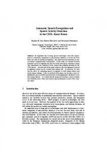
(see Fig. 9.2) is to treat the acoustic waveform as an “noisy” version of the string of words, i.e.. a version that has been passed through a noisy communications channel. This channel introduces “noise” which makes it hard to recognize the “true” string of words. Our goal is then to build a model of the channel so that we can figure out how it modified this “true” sentence and hence recover it. The insight of the noisy channel model is that if we know how the channel distorts the source, we could find the correct source sentence for a waveform by taking every possible sentence in the language, running each sentence through our noisy channel model, and seeing if it matches the output. We then select the best matching source sentence as our desired source sentence. noisy sentence

source sentence

If music be the food of love...

NOISY CHANNEL

DECODER

?Alice was beginning to get... ?Every happy family... ?In a hole in the ground... ?If music be the food of love... ?If music be the foot of dove... ...

guess at original sentence If music be the food of love...

Figure 9.2 The noisy channel model. We search through a huge space of potential “source” sentences and choose the one which has the highest probability of generating the “noisy” sentence. We need models of the prior probability of a source sentence (N-grams), the probability of words being realized as certain strings of phones (HMM lexicons), and the probability of phones being realized as acoustic or spectral features (Gaussian Mixture Models).

BAYESIAN

Implementing the noisy-channel model as we have expressed it in Fig. 9.2 requires solutions to two problems. First, in order to pick the sentence that best matches the noisy input we will need a complete metric for a “best match”. Because speech is so variable, an acoustic input sentence will never exactly match any model we have for this sentence. As we have suggested in previous chapters, we will use probability as our metric. This makes the speech recognition problem a special case of Bayesian inference, a method known since the work of Bayes (1763). Bayesian inference or Bayesian classification was applied successfully by the 1950s to language problems like optical character recognition (Bledsoe and Browning, 1959) and to authorship attribution tasks like the seminal work of Mosteller and Wallace (1964) on determining the authorship of the Federalist papers. Our goal will be to combine various probabilistic models to get a complete estimate for the probability of a noisy acoustic observation-sequence given a candidate source sentence. We can then search through the space of all sentences, and choose the source sentence with the highest probability. Second, since the set of all English sentences is huge, we need an efficient algorithm that will not search through all possible sentences, but only ones that have a good chance of matching the input. This is the decoding or search problem, which we have already explored with the Viterbi decoding algorithm for HMMs in Ch. 5 and Ch. 6. Since the search space is so large in speech recognition, efficient search is an important part of the task, and we will focus on a number of areas in search. In the rest of this introduction we will introduce the probabilistic or Bayesian

Section 9.1.

Speech Recognition Architecture

5

model for speech recognition (or more accurately re-introduce it, since we first used the model in our discussions of part-of-speech tagging in Ch. 5). We then introduce the various components of a modern HMM-based ASR system. We now turn to our probabilistic implementation of the noisy channel intuition, which should be familiar from Ch. 5. The goal of the probabilistic noisy channel architecture for speech recognition can be summarized as follows: “What is the most likely sentence out of all sentences in the language L given some acoustic input O?”

D RA FT

We can treat the acoustic input O as a sequence of individual “symbols” or “observations” (for example by slicing up the input every 10 milliseconds, and representing each slice by floating-point values of the energy or frequencies of that slice). Each index then represents some time interval, and successive oi indicate temporally consecutive slices of the input (note that capital letters will stand for sequences of symbols and lower-case letters for individual symbols):

(9.1)

O = o1 , o2 , o3 , . . . , ot

Similarly, we treat a sentence as if it were composed of a string of words:

(9.2)

W = w1 , w2 , w3 , . . . , wn

Both of these are simplifying assumptions; for example dividing sentences into words is sometimes too fine a division (we’d like to model facts about groups of words rather than individual words) and sometimes too gross a division (we need to deal with morphology). Usually in speech recognition a word is defined by orthography (after mapping every word to lower-case): oak is treated as a different word than oaks, but the auxiliary can (“can you tell me. . . ”) is treated as the same word as the noun can (“i need a can of. . . ” ). The probabilistic implementation of our intuition above, then, can be expressed as follows:

(9.3)

Wˆ = argmax P(W |O) W ∈L

Recall that the function argmaxx f (x) means “the x such that f(x) is largest”. Equation (9.3) is guaranteed to give us the optimal sentence W ; we now need to make the equation operational. That is, for a given sentence W and acoustic sequence O we need to compute P(W |O). Recall that given any probability P(x|y), we can use Bayes’ rule to break it down as follows:

(9.4)

P(x|y) =

P(y|x)P(x) P(y)

We saw in Ch. 5 that we can substitute (9.4) into (9.3) as follows: (9.5)

ˆ = argmax P(O|W )P(W ) W P(O) W ∈L

6

Chapter 9.


D RA FT

The probabilities on the right-hand side of (9.5) are for the most part easier to compute than P(W |O). For example, P(W ), the prior probability of the word string itself is exactly what is estimated by the n-gram language models of Ch. 4. And we will see below that P(O|W ) turns out to be easy to estimate as well. But P(O), the probability of the acoustic observation sequence, turns out to be harder to estimate. Luckily, we can ignore P(O) just as we saw in Ch. 5. Why? Since we are maximizing )P(W ) over all possible sentences, we will be computing P(O|W for each sentence in the P(O) language. But P(O) doesn’t change for each sentence! For each potential sentence we are still examining the same observations O, which must have the same probability P(O). Thus: (9.6)

LANGUAGE MODEL ACOUSTIC MODEL

(9.7)

P(O|W )P(W ) Wˆ = argmax = argmax P(O|W ) P(W ) P(O) W ∈L W ∈L

To summarize, the most probable sentence W given some observation sequence O can be computed by taking the product of two probabilities for each sentence, and choosing the sentence for which this product is greatest. The general components of the speech recognizer which compute these two terms have names; P(W ), the prior probability, is computed by the language model. while P(O|W ), the observation likelihood, is computed by the acoustic model. likelihood prior z }| { z }| { Wˆ = argmax P(O|W ) P(W ) W ∈L

The language model (LM) prior P(W ) expresses how likely a given string of words is to be a source sentence of English. We have already seen in Ch. 4 how to compute such a language model prior P(W ) by using N-gram grammars. Recall that an N-gram grammar lets us assign a probability to a sentence by computing:

(9.8)

P(wn1 ) ≈

n Y

k=1

P(wk |wk−1 k−N+1 )

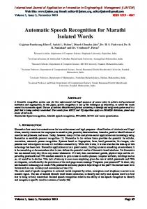
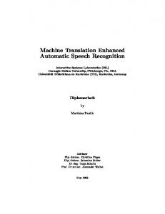
This chapter will show how the HMM we covered in Ch. 6 can be used to build an Acoustic Model (AM) which computes the likelihood P(O|W ). Given the AM and LM probabilities, the probabilistic model can be operationalized in a search algorithm so as to compute the maximum probability word string for a given acoustic waveform. Fig. 9.3 shows a rough block diagram of how the computation of the prior and likelihood fits into a recognizer decoding a sentence. We can see further details of the operationalization in Fig. 9.4, which shows the components of an HMM speech recognizer as it processes a single utterance. The figure shows the recognition process in three stages. In the feature extraction or signal processing stage, the acoustic waveform is sampled into frames (usually of 10, 15, or 20 milliseconds) which are transformed into spectral features. Each time window is thus represented by a vector of around 39 features representing this spectral information as well as information about energy and spectral change. Sec. 9.3 gives an (unfortunately brief) overview of the feature extraction process.

Applying the Hidden Markov Model to Speech

7

D RA FT

Section 9.2.

Figure 9.3 A block diagram of a speech recognizer decoding a single sentence, showing the integration of P(W ) and P(O|W ).

In the acoustic modeling or phone recognition stage, we compute the likelihood of the observed spectral feature vectors given linguistic units (words, phones, subparts of phones). For example, we use Gaussian Mixture Model (GMM) classifiers to compute for each HMM state q, corresponding to a phone or subphone, the likelihood of a given feature vector given this phone p(o|q). A (simplified) way of thinking of the output of this stage is as a sequence of probability vectors, one for each time frame, each vector at each time frame containing the likelihoods that each phone or subphone unit generated the acoustic feature vector observation at that time. Finally, in the decoding phase, we take the acoustic model (AM), which consists of this sequence of acoustic likelihoods, plus an HMM dictionary of word pronunciations, combined with the language model (LM) (generally an N-gram grammar), and output the most likely sequence of words. An HMM dictionary, as we will see in Sec. 9.2, is a list of word pronunciations, each pronunciation represented by a string of phones. Each word can then be thought of as an HMM, where the phones (or sometimes subphones) are states in the HMM, and the Gaussian likelihood estimators supply the HMM output likelihood function for each state. Most ASR systems use the Viterbi algorithm for decoding, speeding up the decoding with wide variety of sophisticated augmentations such as pruning, fast-match, and tree-structured lexicons.

9.2

A PPLYING THE H IDDEN M ARKOV M ODEL TO S PEECH Let’s turn now to how the HMM model is applied to speech recognition. We saw in Ch. 6 that a Hidden Markov Model is characterized by the following components:

Chapter 9.


D RA FT

8

Figure 9.4 Schematic architecture for a (simplified) speech recognizer decoding a single sentence. A real recognizer is more complex since various kinds of pruning and fast matches are needed for efficiency. This architecture is only for decoding; we also need a separate architecture for training parameters.

Q = q1 q2 . . . qN A = a01 a02 . . . an1 . . . ann

O = o1 o2 . . . oN

B = bi (ot )

q0 , qend

a set of states a transition probability matrix A, each ai j representing the P probability of moving from state i to state j, s.t. nj=1 ai j = 1 ∀i

a set of observations, each one drawn from a vocabulary V = v1 , v2 , ..., vV . A set of observation likelihoods:, also called emission probabilities, each expressing the probability of an observation ot being generated from a state i. a special start and end state which are not associated with observations.

Furthermore, the chapter introduced the Viterbi algorithm for decoding HMMs, and the Baum-Welch or Forward-Backward algorithm for training HMMs. All of these facets of the HMM paradigm play a crucial role in ASR. We begin


DIGIT RECOGNITION

BAKIS NETWORK

9

here by discussing how the states, transitions, and observations map into the speech recognition task. We will return to the ASR applications of Viterbi decoding in Sec. 9.6. The extensions to the Baum-Welch algorithms needed to deal with spoken language are covered in Sec. 9.4 and Sec. 9.7. Recall the examples of HMMs we saw earlier in the book. In Ch. 5, the hidden states of the HMM were parts-of-speech, the observations were words, and the HMM decoding task mapped a sequence of words to a sequence of parts-of-speech. In Ch. 6, the hidden states of the HMM were weather, the observations were ‘ice-cream consumptions’, and the decoding task was to determine the weather sequence from a sequence of ice-cream consumption. For speech, the hidden states are phones, parts of phones, or words, each observation is information about the spectrum and energy of the waveform at a point in time, and the decoding process maps this sequence of acoustic information to phones and words. The observation sequence for speech recognition is a sequence of acoustic feature vectors. Each acoustic feature vector represents information such as the amount of energy in different frequency bands at a particular point in time. We will return in Sec. 9.3 to the nature of these observations, but for now we’ll simply note that each observation consists of a vector of 39 real-valued features indicating spectral information. Observations are generally drawn every 10 milliseconds, so 1 second of speech requires 100 spectral feature vectors, each vector of length 39. The hidden states of Hidden Markov Models can be used to model speech in a number of different ways. For small tasks, like digit recognition, (the recognition of the 10 digit words zero through nine), or for yes-no recognition (recognition of the two words yes and no), we could build an HMM whose states correspond to entire words. For most larger tasks, however, the hidden states of the HMM correspond to phone-like units, and words are sequences of these phone-like units. Let’s begin by describing an HMM model in which each state of an HMM corresponds to a single phone (if you’ve forgotten what a phone is, go back and look again at the definition in Ch. 7). In such a model, a word HMM thus consists of a sequence of HMM states concatenated together. In the HMMs described in Ch. 6, there were arbitrary transitions between states; any state could transition to any other. This was also in principle true of the HMMs for part-of-speech tagging in Ch. 5; although the probability of some tag transitions was low, any tag could in principle follow any other tag. Unlike in these other HMM applications, HMM models for speech recognition usually do not allow arbitrary transitions. Instead, they place strong constraints on transitions based on the sequential nature of speech. Except in unusual cases, HMMs for speech don’t allow transitions from states to go to earlier states in the word; in other words, states can transition to themselves or to successive states. As we saw in Ch. 6, this kind of left-to-right HMM structure is called a Bakis network. The most common model used for speech is even more constrained, allowing a state to transition only to itself (self-loop) or to a single succeeding state. The use of self-loops allows a single phone to repeat so as to cover a variable amount of the acoustic input. Phone durations vary hugely, dependent on the phone identify, the the speaker’s rate of speech, the phonetic context, and the level of prosodic prominence of the word. Looking at the Switchboard corpus, the phone [aa] varies in length from 7

D RA FT

Section 9.2.

10

Chapter 9.


D RA FT

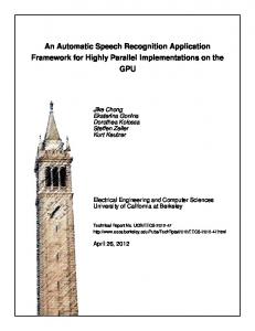
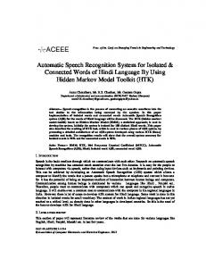
to 387 milliseconds (1 to 40 frames), while the the phone [z] varies in duration from 7 milliseconds to more than 1.3 seconds (130 frames) in some utterances! Self-loops thus allow a single state to be repeated many times. Fig. 9.5 shows a schematic of the structure of a basic phone-state HMM, with self-loops and forward transitions, for the word six.

Figure 9.5 An HMM for the word six, consisting of four emitting states and two nonemitting states, the transition probabilities A, the observation probabilities B, and a sample observation sequence.

MODEL

PHONE MODEL HMM STATE

For very simple speech tasks (recognizing small numbers of words such as the 10 digits), using an HMM state to represent a phone is sufficient. In general LVCSR tasks, however, a more fine-grained representation is necessary. This is because phones can last over 1 second, i.e., over 100 frames, but the 100 frames are not acoustically identical. The spectral characteristics of a phone, and the amount of energy, vary dramatically across a phone. For example, recall from Ch. 7 that stop consonants have a closure portion, which has very little acoustic energy, followed by a release burst. Similarly, diphthongs are vowels whose F1 and F2 change significantly. Fig. 9.6 shows these large changes in spectral characteristics over time for each of the two phones in the word “Ike”, ARPAbet [ay k]. To capture this fact about the non-homogeneous nature of phones over time, in LVCSR we generally model a phone with more than one HMM state. The most common configuration is to use three HMM states, a beginning, middle, and end state. Each phone thus consists of 3 emitting HMM states instead of one (plus two nonemitting states at either end), as shown in Fig. 9.7. It is common to reserve the word model or phone model to refer to the entire 5-state phone HMM, and use the word HMM state (or just state for short) to refer to each of the 3 individual subphone HMM states. To build a HMM for an entire word using these more complex phone models, we can simply replace each phone of the word model in Fig. 9.5 with a 3-state phone HMM. We replace the non-emitting start and end states for each phone model with transitions directly to the emitting state of the preceding and following phone, leaving only two non-emitting states for the entire word. Fig. 9.8 shows the expanded word. In summary, an HMM model of speech recognition is parameterized by:

Section 9.2.


11

D RA FT

Frequency (Hz)

5000

0 0.48152

ay

k

0.937203

Time (s)

Figure 9.6 The two phones of the word ”Ike”, pronounced [ay k]. Note the continuous changes in the [ay] vowel on the left, as F2 rises and F1 falls, and the sharp differences between the silence and release parts of the [k] stop.

Figure 9.7 A standard 5-state HMM model for a phone, consisting of three emitting states (corresponding to the transition-in, steady state, and transition-out regions of the phone) and two non-emitting states.

Figure 9.8 A composite word model for “six”, [s ih k s], formed by concatenating four phone models, each with three emitting states.

Q = q1 q2 . . . qN A = a01 a02 . . . an1 . . . ann

a set of states corresponding to subphones a transition probability matrix A, each ai j representing the probability for each subphone of taking a self-loop or going to the next subphone.

B = bi (ot )

A set of observation likelihoods:, also called emission probabilities, each expressing the probability of a cepstral feature vector (observation ot ) being generated from subphone state i.

12

Chapter 9.


D RA FT

Another way of looking at the A probabilities and the states Q is that together they represent a lexicon: a set of pronunciations for words, each pronunciation consisting of a set of subphones, with the order of the subphones specified by the transition probabilities A. We have now covered the basic structure of HMM states for representing phones and words in speech recognition. Later in this chapter we will see further augmentations of the HMM word model shown in Fig. 9.8, such as the use of triphone models which make use of phone context, and the use of special phones to model silence. First, though, we need to turn to the next component of HMMs for speech recognition: the observation likelihoods. And in order to discuss observation likelihoods, we first need to introduce the actual acoustic observations: feature vectors. After discussing these in Sec. 9.3, we turn in Sec. 9.4 the acoustic model and details of observation likelihood computation. We then re-introduce Viterbi decoding and show how the acoustic model and language model are combined to choose the best sentence.

9.3

F EATURE E XTRACTION

THIS SECTION STILL TO BE WRITTEN. IT WILL START FROM DIGITIZATION AND WAVE FILE FORMATS AND GO THROUGH PRODUCTION OF MFCC FILES.

9.4

C OMPUTING ACOUSTIC L IKELIHOODS

The last section showed how we can extract MFCC features representing spectral information from a wavefile, and produce a 39-dimensional vector every 10 milliseconds. We are now ready to see how to compute the likelihood of these feature vectors given an HMM state. Recall from Ch. 6 that this output likelihood is computed by the B probability function of the HMM. Given an individual state qi and an observation ot , the observation likelihoods in B matrix gave us p(ot |qi ), which we called bt (i). For part-of-speech tagging in Ch. 5, each observation ot is a discrete symbol (a word) and we can compute the likelihood of an observation given a part-of-speech tag just by counting the number of times a given tag generates a given observation in the training set. But for speech recognition, MFCC vectors are real-valued numbers; we can’t compute the likelihood of a given state (phone) generating an MFCC vector by counting the number of times each such vector occurs (since each one is likely to be unique). In both decoding and training, we need an observation likelihood function that can compute p(ot |qi ) on real-valued observations. In decoding, we are given an observation ot and we need to produce the probability p(ot |qi ) for each possible HMM state, so we can choose the most likely sequence of states. Once we have this observation likelihood B function, we need to figure out how to modify the Baum-Welch algorithm of Ch. 6 to train it as part of training HMMs.

Section 9.4.

Computing Acoustic Likelihoods

13

9.4.1 Vector Quantization

VECTOR QUANTIZATION

D RA FT

V

One way to make MFCC vectors look like symbols that we could count is to build a mapping function that maps each input vector into one of a small number of symbols. Then we could just compute probabilities on these symbols by counting, just as we did for words in part-of-speech tagging. This idea of mapping input vectors to discrete quantized symbols is called vector quantization or VQ (Gray, 1984). Although vector quantization is too simple to act as the acoustic model in modern LVCSR systems, it is a useful pedagogical step, and plays an important role in various areas of ASR, so we use it to begin our discussion of acoustic modeling. In vector quantization, we create the small symbol set by mapping each training feature vector into a small number of classes, and then we represent each class by a discrete symbol. More formally, a vector quantization system is characterized by a codebook, a clustering algorithm, and a distance metric. A codebook is a list of possible classes, a set of symbols constituting a vocabulary V = {v1 , v2 , ..., vn }. For each symbol vk in the codebook we list a prototype vector, also known as a codeword, which is a specific feature vector. For example if we choose to use 256 codewords we could represent each vector by a value from 0 to 255; (this is referred to as 8-bit VQ, since we can represent each vector by a single 8-bit value). Each of these 256 values would be associated with a prototype feature vector. The codebook is created by using a clustering algorithm to cluster all the feature vectors in the training set into the 256 classes. Then we chose a representative feature vector from the cluster, and make it the prototype vector or codework for that cluster. K-means clustering is often used, but we won’t define clustering here; see Huang et al. (2001) or Duda et al. (2000) for detailed descriptions. Once we’ve built the codebook, for each incoming feature vector, we compare it to each of the 256 prototype vectors, select the one which is closest (by some distance metric), and replace the input vector by the index of this prototype vector. A schematic of this process is shown in Fig. 9.9. The advantage of VQ is that since there are a finite number of classes, for each class vk , we can compute the probability that it is generated by a given HMM state/subphone by simply counting the number of times it occurs in some training set when labeled by that state, and normalizing. Both the clustering process and the decoding process require a distance metric or distortion metric, that specifies how similar two acoustic feature vectors are. The distance metric is used to build clusters, to find a prototype vector for each cluster, and to compare incoming vectors to the prototypes. The simplest distance metric for acoustic feature vectors is Euclidean distance. Euclidean distance is the distance in N-dimensional space between the two points defined by the two vectors. In practice what we refer to as Euclidean distance is actually the square of the distance. Thus given a vector x and a vector y of length D, the (square of the) Euclidean distance between them is defined as:

CODEBOOK

PROTOTYPE VECTOR

CODEWORD

CLUSTERING

K-MEANS CLUSTERING

DISTANCE METRIC

EUCLIDEAN DISTANCE

(9.9)

deuclidean(x, y) =

D X (xi − yi )2 i=1

Chapter 9.


D RA FT

14

Figure 9.9 Schematic architecture of the (trained) vector quantization (VQ) process for choosing a symbol vq for each input feature vector. The vector is compared to each codeword in the codebook, the closest entry (by some distance metric) is selected, and the index of the closest codeword is output.

The (squared) Euclidean distance described in (9.9) (and shown for two dimensions in Fig. 9.10) is also referred to as the sum-squared error, and can also be expressed using the vector transpose operator as:

(9.10)

deuclidean(x, y) = (x − y)T (x − y)

Figure 9.10 Euclidean distance in two dimensions; by the Pythagorean theorem, the distance between two points in a plane x = (x1, y1) and y = (x2, y2) d(x, y) = p (x1 − x2 )2 + (y1 − y2 )2 .

The Euclidean distance metric assumes that each of the dimensions of a feature vector are equally important. But actually each of the dimensions have very different variances. If a dimension tends to have a lot of variance, then we’d like it to count less in the distance metric; a large difference in a dimension with low variance should

Section 9.4.

MAHALANOBIS DISTANCE


15

count more than a large difference in a dimension with high variance. A slightly more complex distance metric, the Mahalanobis distance, takes into account the different variances of each of the dimensions. If we assume that each dimension i of the acoustic feature vectors has a variance σ2i , then the Mahalanobis distance is: dmahalanobis(x, y) =

(9.11)

D X (xi − yi )2 i=1

σ2i

D RA FT

For those readers with more background in linear algebra here’s the general form of Mahalanobis distance, which includes a full covariance matrix (covariance matrices will be defined below):

(9.12)

dmahalanobis(x, y) = (x − y)T Σ−1 (x − y)

In summary, when decoding a speech signal, to compute an acoustic likelihood of a feature vector ot given an HMM state q j using VQ, we compute the Euclidean or Mahalanobis distance between the feature vector and each of the N codewords, choose the closest codeword, getting the codeword index vk . We then look up the likelihood of the codeword index vk given the HMM state j in the pre-computed B likelihood matrix defined by the HMM:

(9.13)

bˆ j (ot ) = b j (vk ) s.t. vk is codeword of closest vector to ot

Since VQ is so rarely used, we don’t use up space here giving the equations for modifying the EM algorithm to deal with VQ data; instead, we defer discussion of EM training of continuous input parameters to the next section, when we introduce Gaussians.

9.4.2 Gaussian PDFs

PROBABILITY DENSITY FUNCTION

GAUSSIAN MIXTURE MODEL GMM

Vector quantization has the advantage of being extremely easy to compute and requires very little storage. Despite these advantages, vector quantization is simply not a good model of speech. A small number of codewords is insufficient to capture the wide variability in the speech signal. Speech is simply not a categorical, symbolic process. Modern speech recognition algorithms therefore do not use vector quantization to compute acoustic likelihoods. Instead, they are based on computing observation probabilities directly on the real-valued, continuous input feature vector. These acoustic models are based on computing a probability density function or pdf over a continuous space. By far the most common method for computing acoustic likelihoods is the Gaussian Mixture Model (GMM) pdfs, although neural networks, support vector machines (SVMs) and conditional random fields (CRFs) are also used. Let’s begin with the simplest use of Gaussian probability estimators, slowly building up the more sophisticated models that are used. Univariate Gaussians

GAUSSIAN NORMAL DISTRIBUTION

The Gaussian distribution, also known as the normal distribution, is the bell-curve

16

Chapter 9.

MEAN VARIANCE


function familiar from basic statistics. A Gaussian distribution is a function parameterized by a mean, or average value, and a variance, which characterizes the average spread or dispersal from the mean. We will use µ to indicate the mean, and σ2 to indicate the variance, giving the following formula for a Gaussian function: 1 (x − µ)2 f (x|µ, σ) = √ ) exp(− 2σ2 2πσ2

(9.14)

1.6

D RA FT

m=0,s=.5 m=1,s=1 m=−1,s=0.2 m=0,s=0.3

1.4 1.2 1

0.8

0.6 0.4 0.2

0 −4

Figure 9.11

−3

−2

−1

0

1

2

3

4

Gaussian functions with different means and variances.

Recall from basic statistics that the mean of a random variable X is the expected value of X. For a discrete variable X, this is the weighted sum over the values of X (for a continuous variable, it is the integral): µ = E(X) =

(9.15)

N X

p(Xi )Xi

i=1

The variance of a random variable X is the squared average deviation from the

mean:

(9.16)

σ2 = E(Xi − E(X))2 ) =

N X i=1

p(Xi )(Xi − E(X))2

When a Gaussian function is used as a probability density function, the area under the curve is constrained to be equal to one. Then the probability that a random variable takes on any particular range of values can be computed by summing the area

Section 9.4.


17

0.4 0.35 ← P(shaded region) = .341

Probability Density

0.3 0.25

0.2 0.15

D RA FT

0.1 0.05

0 −4

−3

−2

−1

0

1

2

3

4

Figure 9.12 A Gaussian probability density function, showing a region from 0 to 1 with a total probability of .341. Thus for this sample Gaussian, the probability that a value on the X axis lies between 0 and 1 is .341.

under the curve for that range of values. Fig. 9.12 shows the probability expressed by the area under an interval of a Gaussian. We can use a univariate Gaussian pdf to estimate the probability that a particular HMM state j generates the value of a single dimension of a feature vector by assuming that the possible values of (this one dimension of the) observation feature vector ot are normally distributed. In other words we represent the observation likelihood function b j (ot ) for one dimension of the acoustic vector as a Gaussian. Taking, for the moment, our observation as a single real valued number (a single cepstral feature), and assuming that each HMM state j has associated with it a mean value µ j and variance σ2j , we compute the likelihood b j (ot ) via the equation for a Gaussian pdf:

(9.17)

(ot − µ j )2 b j (ot ) = q exp − 2σ2j 2πσ2j 1

!

Equation (9.17) shows us how to compute b j (ot ), the likelihood of an individual acoustic observation given a single univariate Gaussian from state j with its mean and variance. We can now use this probability in HMM decoding. But first we need to solve the training problem; how do we compute this mean and variance of the Gaussian for each HMM state qi ? Let’s start by imagining the simpler situation of a completely labeled training set, in which each acoustic observation was labeled with the HMM state that produced it. In such a training set, we could compute the mean of each state just taking the average of the values for each ot that corresponded to state i, as show in (9.18). The variance could just be computed from

18

Chapter 9.


the sum-squared error between each observation and the mean, as shown in (9.19). (9.18)

σˆ 2j =

T 1X ot s.t. qt is state i T

1 T

t=1 T X t=1

(ot − µi )2 s.t. qt is state i

But since states are hidden in an HMM, we don’t know exactly which observation vector ot was produced by which state. What we would like to do is assign each observation vector ot to every possible state i, prorated by the probability that the HMM was in state i at time t. Luckily, we already know how to do this prorating; the probability of being in state i at time t was defined in Ch. 6 as ξt (i), and we saw how to compute ξt (i) as part of the Baum-Welch algorithm using the forward and backward probabilities. Baum-Welch is an iterative algorithm, and we will need to do the probability computation of ξt (i) iteratively since getting a better observation probability b will also help us be more sure of the probability ξ of being in a state at a certain time. Thus we give equations for computing an updated mean and variance µˆ and σˆ2 : PT ξt (i)ot µˆ i = Pt=1 T t=1 ξt (i) PT 2 t=1 ξt (i)(ot − µi ) σˆ 2i = PT t=1 ξt (i)

D RA FT

(9.19)

µˆ i =

(9.20)

(9.21)

Equations (9.20) and (9.21) are then used in the forward-backward (Baum-Welch) training of the HMM. As we will see, the values of µi and σi are first set to some initial estimate, which is then re-estimated until the numbers converge.

Multivariate Gaussians

Equation (9.17) shows how to use a Gaussian to compute an acoustic likelihood for a single cepstral feature. Since an acoustic observation is a vector of 39 features, we’ll need to use a multivariate Gaussian, which allows us to assign a probability to a 39valued vector. Where a univariate Gaussian is defined by a mean µ and a variance σ2 , a multivariate Gaussian is defined by a mean vector ~µ of dimensionality D and a covariance matrix Σ, defined below. For a typical cepstral feature vector in LVCSR, D is 39:

(9.22)

(9.23)

1 f (~x|~µ, Σ) = p exp (x − µ)T Σ−1 (ot − µ j ) 2π|Σ| The covariance matrix Σ captures the variance of each dimension as well as the covariance between any two dimensions. Recall again from basic statistics that the covariance of two random variables X and Y is the expected value of the product of their average deviations from the mean: Σ = E[(X − E(X))(Y − E(Y )]) =

N X i=1

p(XiYi )(Xi − E(X))(Yi − E(Y ))

Section 9.4.


19

Thus for a given HMM state with mean vector µ j and covariance matrix Σ j , and a given observation vector ot , the multivariate Gaussian probability estimate is: 1 b j (ot ) = p exp (ot − µ j )T Σ−1 (o − µ ) t j j 2π|Σ j|

(9.24)

D RA FT

The covariance matrix Σ j expresses the variance between each pair of feature dimensions. Suppose we made the simplifying assumption that features in different dimensions did not covary, i.e., that there was no correlation between the variances of different dimensions of the feature vector. In this case, we could simply keep a distinct variance for each feature dimension. It turns out that keeping a separate variance for each dimension is equivalent to having a covariance matrix that is diagonal, i.e. non-zero elements only appear along the main diagonal of the matrix. The main diagonal of such a diagonal covariance matrix contains the variances of each dimension, σ21 , σ22 , ...σ2D ; Let’s look at some illustrations of multivariate Gaussians, focusing on the role of the full versus diagonal covariance matrix. We’ll explore a simple multivariate Gaussian with only 2 dimensions, rather than the 39 that are typical in ASR. Fig. 9.13 shows three different multivariate Gaussians in two dimensions. The leftmost figure shows a Gaussian with a diagonal covariance matrix, in which the variances of the two dimensions are equal. Fig. 9.14 shows 3 contour plots corresponding to the Gaussians in Fig. 9.13; each is a slice through the Gaussian. The leftmost graph in Fig. 9.14 shows a slice through the diagonal equal-variance Gaussian. The slice is circular, since the variances are equal in both the X and Y directions.

DIAGONAL

0.35

0.35

0.3

0.3

0.25

0.25

1

0.8

0.2

0.2

0.6

0.15

0.15

0.4

0.1

0.1

0.05

0.05

0 4

0 4

2

4

2

0

0

−2

−2

−4

−4

(a)

0.2 0 4

2

4

2

0

0

−2

−2

−4

2

4 2

0

0

−2

−2

−4

−4

(b)

−4

(c)

Figure 9.13 Three different multivariate Gaussians in two dimensions. The first two have diagonal covariance matrices, one with equal variance in the two dimensions 1 0 .6 0 , the second with different variances in the two dimensions, , and the 0 1 0 2 third with non-zero elements in the off-diagonal of the covariance matrix:

1 .8 . .8 1

The middle figure in Fig. 9.13 shows a Gaussian with a diagonal covariance matrix, but where the variances are not equal. It is clear from this figure, and especially from the contour slice show in Fig. 9.14, that the variance is more than 3 times greater in one dimension than the other.

20

Chapter 9.


3

3

3

2

2

2

1

1

1

0

0

0

−1

−1

−1

−2

−2

−2

−3 −3

−3 −3

−2

−1

0

1

2

3

(a)

−2

−1

0

1

2

3

−3 −3

−2

(b)

−1

0

1

2

3

(c)

D RA FT

Figure 9.14 The same three multivariate Gaussians as in the previous figure. From left to right, a diagonal covariance matrix with equal variance, diagonal with unequal variance, and and nondiagonal covariance. With non-diagonal covariance, knowing the value on dimension X tells you something about the value on dimension Y.

The rightmost graph in Fig. 9.13 and Fig. 9.14 shows a Gaussian with a nondiagonal covariance matrix. Notice in the contour plot in Fig. 9.14 that the contour is not lined up with the two axes, as it is in the other two plots. Because of this, knowing the value in one dimension can help in predicting the value in the other dimension. Thus having a non-diagonal covariance matrix allows us to model correlations between the values of the features in multiple dimensions. A Gaussian with a full covariance matrix is thus a more powerful model of acoustic likelihood than one with a diagonal covariance matrix. And indeed, speech recognition performance is better using full-covariance Gaussians than diagonal-covariance Gaussians. But there are two problems with full-covariance Gaussians that makes them difficult to use in practice. First, they are slow to compute. A full covariance matrix has D2 parameters, where a diagonal covariance matrix has only D. This turns out to make a large difference in speed in real ASR systems. Second, a full covariance matrix has many more parameters and hence requires much more data to train than a diagonal covariance matrix. Using a diagonal covariance model means we can save room for using our parameters for other things like triphones. For this reason, in practice most ASR systems use diagonal covariance. We will assume diagonal covariance for the remainder of this section. Equation (9.24) can thus be simplified to the version in (9.25) in which instead of a covariance matrix, we simply keep a mean and variance for each dimension. Equation (9.25) thus describes how to estimate the likelihood b j (ot ) of a D-dimensional feature vector ot given HMM state j, using a diagonal-covariance multivariate Gaussian.

(9.25)

D Y

1 1 (otd − µ jd )2 q ] b j (ot ) = exp − [ 2 σ jd 2 2πσ2jd d=1

Training a diagonal-covariance multivariate Gaussian is a simple generalization of training univariate Gaussians. We’ll do the same Baum-Welch training, where we use the value of ξt (i) to tell us the likelihood of being in state i at time t. Indeed, we’ll use exactly same equation as in (9.21), except that now we are dealing with vectors instead of scalars; the observation ot is a vector of cepstral features, the mean vector~µ

Section 9.4.


21

~2 is a vector of cepstral variances. is a vector of cepstral means, and the variance vector σ i

µˆ i =

(9.26)

σˆ 2i =

(9.27)

Gaussian Mixture Models

PT

Pt=1 T

ξt (i)ot

t=1 ξt (i)

PT

t=1 ξt (i)(ot − µi )(ot PT t=1 ξt (i)

− µi )T

D RA FT

The previous subsection showed that we can use a multivariate Gaussian model to assign a likelihood score to an acoustic feature vector observation. This models each dimension of the feature vector as a normal distribution. But a particular cepstral feature might have a very non-normal distribution; the assumption of a normal distribution may be too strong an assumption. For this reason, we often model the observation likelihood not with a single multivariate Gaussian, but with a weighted mixture of multivariate Gaussians. Such a model is called a Gaussian Mixture Model or GMM. Equation (9.28) shows the equation for the GMM function; the resulting function is the sum of M Gaussians. Fig. 9.15 shows an intuition of how a mixture of Gaussians can model arbitrary functions.

GAUSSIAN MIXTURE MODEL GMM

Figure 9.15 Add figure here showing a mixture of 3 guassians covering a function with 3 lumps; SHOW differences in VARIANCE, MEAN, AND WEIGHT.

(9.28)

f (x|µ, Σ) =

M X

1 ck p exp[(x − µk )T Σ−1 (x − µk )] 2π|Σk | k=1

Equation (9.29) shows the definition of the output likelihood function b j (ot )

(9.29)

b j (ot ) =

M X

1 c jm p exp[(x − µ jm )T Σ−1 jm (ot − µ jm )] 2π|Σ | jm m=1

Let’s turn to training the GMM likelihood function. This may seem hard to do; how can we train a GMM model if we don’t know in advance which mixture is supposed to account for which part of each distribution? Recall that a single multivariate Gaussian could be trained even if we didn’t know which state accounted for each output, simply by using the Baum-Welch algorithm to tell us the likelihood of being in each state j at time t. It turns out the same trick will work for GMMs; we can use Baum-Welch to tell us the probability of a certain mixture accounting for the observation, and iteratively update this probability. We used the ξ function above to help us compute the state probability. By analogy with this function, let’s define ξtm ( j) to mean the probability of being in state j at time t with the mth mixture component accounting for the output observation ot . We can compute ξtm ( j) as follows:

22

Chapter 9.

ξtm ( j) =

(9.30)

P


i=1 Nαt−1 ( j)ai j c jm b jm (ot )βt ( j)

αT (F)

Now if we had the values of ξ from a previous iteration of Baum-Welch, we can use ξtm ( j) to recompute the mean, mixture weight, and covariance using the following equations: PT

ξtm (i)ot µˆ im = PT t=1 PM m=1 ξtm (i) t=1 PT ξtm (i) cîm = PT t=1 PM t=1 k=1 ξtk (i) PT T t=1 ξt (i)(ot − µim )(ot − µim ) Σˆ im = PT PM k=1 ξtm (i) t=1

D RA FT

(9.31)

(9.32)

(9.33)

9.4.3 Probabilities, log probabilities and distance functions

LOGPROB

(9.34)

Up to now, all the equations we have given for acoustic modeling have used probabilities. It turns out, however, that a log probability (or logprob) is much easier to work with than a probability. Thus in practice throughout speech recognition (and related fields) we compute log-probabilities rather than probabilities. One major reason that we can’t use probabilities is numeric underflow. To compute a likelihood for a whole sentence, say, we are multiplying many small probability values, one for each 10ms frame. Multiplying many probabilities results in smaller and smaller numbers, leading to underflow. The log of a small number like .00000001 = 10−8, on the other hand, is a nice easy-to-work-with-number like −8. A second reason to use log probabilities is computational speed. Instead of multiplying probabilities, we add log-probabilities, and adding is faster than multiplying. Logprobabilities are particularly efficient when we are using Gaussian models, since we can avoid exponentiating. Thus for example for a single multivariate diagonal-covariance Gaussian model, instead of computing: ! D Y 1 1 (otd − µ jd )2 q b j (ot ) = exp − 2 2 σ2jd 2πσ d=1 jd

we would compute

(9.35)

" # D 2 (o − µ ) 1X td jd log b j (ot ) = − log(2π) + σ2jd + 2 σ2jd d=1

(9.36)

With some rearrangement of terms, we can rewrite this equation to pull out a constant C: D 1 X (otd − µ jd )2 log b j (ot ) = C − 2 σ2jd d=1

Section 9.5.

The Lexicon and Language Model

23

where C can be precomputed: D

(9.37)

C=−

1X log(2π) + σ2jd 2 d=1

D RA FT

In summary, computing acoustic models in log domain means a much simpler computation, much of which can be precomputed for speed. The perceptive reader may have noticed that equation (9.36) looks very much like the equation for Mahalanobis distance (9.11). Indeed, one way to think about Gaussian logprobs is as just a weighted distance metric. A further point about Gaussian pdfs, for those readers with calculus. Although the equations for observation likelihood such as (9.17) are motivated by the use of Gaussian probability density functions, the values they return for the observation likelihood, b j (ot ), are not technically probabilities; they may in fact be greater than one. This is because we are computing the value of b j (ot ) at a single point, rather than integrating over a region. While the total area under the Gaussian PDF curve is constrained to one, the actual value at any point could be greater than one. (Imagine a very tall skinny Gaussian; the value could be greater than one at the center, although the area under the curve is still 1.0). If we were integrating over a region, we would be multiplying each point by its width dx, which would bring the value down below one. The fact that the Gaussian estimate is not a true probability doesn’t matter for choosing the most likely HMM state, since we are comparing different Gaussians, each of which is missing this dx factor. In summary, the last few subsections introduced Gaussian models for acoustic training in speech recognition. Beginning with simple univariate Gaussian, we extended first to multivariate Gaussians to deal with the multidimensionality acoustic feature vectors. We then introduced the diagonal covariance simplification of Gaussians, and then introduced Gaussians mixtures (GMMs).

9.5

T HE L EXICON AND L ANGUAGE M ODEL

Since previous chapters had extensive discussions of the N-gram language model (Ch. 4) and the pronunciation lexicon (Ch. 7), in this section we just briefly recall them to the reader. Language models for LVCSR tend to be trigrams or even fourgrams; good toolkits are available to build and manipulate them (Stolcke, 2002; Young et al., 2005). Bigrams and unigram grammars are rarely used for large-vocabulary applications. Since trigrams require huge amounts of space, however, language models for memory-constrained applications like cell phones tend to use smaller contexts. As we will discuss in Ch. 23, some simple dialogue applications take advantage of their limited domain to use very simple finite state or weighted-finite state grammars. Lexicons are simply lists of words, with a pronunciation for each word expressed as a phone sequence. Publicly available lexicons like the CMU dictionary (CMU, 1993) can be used to extract the 64,000 word vocabularies commonly used for LVCSR. Most words have a single pronunciation, although some words such as homonyms and

24

Chapter 9.


frequent function words may have more; the average number of pronunciations per word in most LVCSR systems seems to range from 1 to 2.5. Sec. 9.12.3 discusses the issue of pronunciation modeling.

S EARCH AND D ECODING We are now very close to having described all the parts of a complete speech recognizer. We have shown how to extract cepstral features for a frame, and how to compute the acoustic likelihood b j (ot ) for that frame. We also know how to represent lexical knowledge, that each word HMM is composed of a sequence of phones, and each of phone of set of subphone states. Finally, in Ch. 4 we showed how to use N-grams to build a model of word predictability. In this section we show how to combine all of this knowledge to solve the problem of decoding: combining all these probability estimators to produce the most probable string of words. We can phrase the decoding question as: ‘Given a string of acoustic observations, how should we choose the string of words which has the highest posterior probability?’ Recall from the beginning of the chapter the noisy channel model for speech recognition. In this model, we use Bayes rule, with the result that the best sequence of words is the one that maximizes the product of two factors, a language model prior and an acoustic likelihood:

D RA FT

9.6

DECODING

(9.38)

likelihood prior z }| { z }| { Wˆ = argmax P(O|W ) P(W ) W ∈L

LMSF

(9.39)

Now that we have defined both the acoustic model (in this chapter) and language model (in Ch. 4), we are ready to see how to find this maximum probability sequence of words. First, though, it turns out that we’ll need to make a modification to Equation (9.38), because it relies on some incorrect independence assumptions. Recall that we trained a multivariate Gaussian mixture classifier to compute the likelihood of a particular acoustic observation (a frame) given a particular state (subphone). By computing separate classifiers for each acoustic frame and multiplying these probabilities to get the probability of the whole word, we are severely underestimating the probability of each subphone. This is because there is a lot of continuity across frames; if we were to take into account the acoustic context, we would have a greater expectation for a given frame and hence could assign it a higher probability. We must therefore reweight the two probabilities. We do this by add in a language model scaling factor or LMSF, also called the language weight. This factor is an exponent on the language model probability P(W ). Because P(W ) is less than one and the LMSF is greater than one (between 5 and 15, in many systems), this has the effect of decreasing the value of the LM probability: ˆ = argmax P(O|W )P(W )LMSF W W ∈L

Section 9.6.

Search and Decoding

25

Reweighting the language model probability P(W ) in this way requires us to make one more change. This is because P(W ) has a side-effect as a penalty for inserting words. It’s simplest to see this in the case of a uniform language model, where every word in a vocabulary of size |V | has an equal probability |V1 | . In this case, a sentence with N words will have a language model probability of

for a total penalty of of 1 V

N |V | .

1 |V |

for each of the N words,

The larger N is (the more words in the sentence), the more

D RA FT

times this penalty multiplier is taken, and the less probable the sentence will be. Thus if (on average) the language model probability decreases (causing a larger penalty), the decoder will prefer fewer, longer words. If the language model probability increases (larger penalty), the decoder will prefer more shorter words. Thus our use of a LMSF to balance the acoustic model has the side-effect of decreasing the word insertion penalty. To offset this, we need to add back in a separate word insertion penalty:

WORD INSERTION PENALTY

Wˆ = argmax P(O|W )P(W )LMSF WIPN

(9.40)

W ∈L

Since in practice we use logprobs, the goal of our decoder is:

Wˆ = argmax log P(O|W ) + LMSF × log P(W ) + N × logWIP

(9.41)

W ∈L

Now that we have an equation to maximize, let’s look at how to decode. It’s the job of a decoder to simultaneously segment the utterance into words and identify each of these words. This task is made difficult by variation, both in terms of how words are pronounced in terms of phones, and how phones are articulated in acoustic features. Just to give an intuition of the difficulty of the problem imagine a massively simplified version of the speech recognition task, in which the decoder is given a series of discrete phones. In such a case, we would know what each phone was with perfect accuracy, and yet decoding is still difficult. For example, try to decode the following sentence from the (hand-labeled) sequence of phones from the Switchboard corpus (don’t peek ahead!): [ay d ih s hh er d s ah m th ih ng ax b aw m uh v ih ng r ih s en l ih]

The answer is in the footnote.1 The task is hard partly because of coarticulation and fast speech (e.g., [d] for the first phone of just!). But it’s also hard because speech, unlike English writing, has no spaces indicating word boundaries. The true decoding task, in which we have to identify the phones at the same time as we identify and segment the words, is of course much harder. For decoding, we will start with the Viterbi algorithm that we introduced in Ch. 6, in the domain of digit recognition, a simple task with with a vocabulary size of 11 (the numbers one through nine plus zero and oh). Recall the basic components of an HMM model for speech recognition: 1

I just heard something about moving recently.

26

Chapter 9.


a set of states corresponding to subphones a transition probability matrix A, each ai j representing the probability for each subphone of taking a self-loop or going to the next subphone. Together, Q and A implement a pronunciation lexicon, an HMM state graph structure for each word that the system is capable of recognizing.

B = bi (ot )


D RA FT

Q = q1 q2 . . . qN A = a01 a02 . . . an1 . . . ann

The HMM structure for each word comes from a lexicon of word pronunciations. Generally we use an off-the-shelf pronunciation dictionary such as the free CMUdict dictionary described in Ch. 7. Recall from page 9 that the HMM structure for words in speech recognition is a simple concatenation of phone HMMs, each phone consisting of 3 subphone states, where every state has exactly two transitions: a self-loop and a loop to the next phones. Thus the HMM structure for each digit word in our digit recognizer is computed simply by taking the phone string from the dictionary, expanding each phone into 3 subphones, and concatenating together. In addition, we generally add an optional silence phone at the end of each word, allowing the possibility of pausing between words. We usually define the set of states Q from some version of the ARPAbet, augmented with silence phones, and expanded to create three subphones for each phone. The A and B matrices for the HMM are trained by the Baum-Welch algorithm in the embedded training procedure that we will describe in Sec. 9.7. For now we’ll assume that these probabilities have been trained. Fig. 9.16 shows the resulting HMM for digit recognition. Note that we’ve added non-emitting start and end states, with transitions from the end of each word to the end state, and a transition from the end state back to the start state to allow for sequences of digits. Note also the optional silence phones at the end of each word. Digit recognizers often don’t use word probabilities, since in most digit situations (phone numbers or credit card numbers) each digit has an equal probability of appearing. But we’ve included transition probabilities into each word in Fig. 9.16, mainly to show where such probabilities would be for other kinds of recognition tasks. As it happens, there are cases where digit probabilities do matter, such as in addresses (which are often likely to end in 0 or 00) or in cultures where some numbers are lucky and hence more frequent, such as the lucky number ‘8’ in Chinese. Now that we have an HMM, we can use the same forward and Viterbi algorithms that we introduced in Ch. 6. Let’s see how to use the forward algorithm to generate P(O|W ), the likelihood of an observation sequence O given a sequence of words W ; we’ll use the single word “five”. In order to compute this likelihood, we need to sum over all possible sequences of states; assuming five has the states [f], [ay], and [v], a 10-observation sequence includes many sequences such as the following: f ay ay ay ay v

v

v

v

v

Search and Decoding

27

D RA FT

Section 9.6.

Figure 9.16 An HMM for the digit recognition task. A lexicon specifies the phone sequence, and each phone HMM is composed of three subphones each with a Gaussian emission likelihood model. Combining these and adding an optional silence at the end of each word, results in a single HMM for the whole task. Note the transition from the End state to the Start state to allow digit sequences of arbitrary length.

f f f f f f f f f f ...

ay f ay ay ay

ay f ay ay ay

ay ay ay ay ay

ay ay ay ay ay

v ay ay ay ay

v ay ay ay v

v v v ay v

v v v v v

The forward algorithm efficiently sums over this large number of sequences in O(N 2 T ) time. Let’s quickly review the forward algorithm. It is a dynamic programming algorithm, i.e. an algorithm that uses a table to store intermediate values as it builds up the probability of the observation sequence. The forward algorithm computes the observation probability by summing over the probabilities of all possible paths that could generate the observation sequence. Each cell of the forward algorithm trellis αt ( j) or forward[t, j] represents the probability of being in state j after seeing the first t observations, given the automaton

28

Chapter 9.


λ. The value of each cell αt ( j) is computed by summing over the probabilities of every path that could lead us to this cell. Formally, each cell expresses the following probability: αt ( j) = P(o1 , o2 . . . ot , qt = j|λ)

(9.42)

D RA FT

(9.43)

Here qt = j means “the probability that the tth state in the sequence of states is state j”. We compute this probability by summing over the extensions of all the paths that lead to the current cell. For a given state q j at time t, the value αt ( j) is computed as: N−1 X αt ( j) = αt−1 (i)ai j b j (ot ) i=1

The three factors that are multiplied in Eq˙ 9.43 in extending the previous paths to compute the forward probability at time t are: αt−1 (i)

the previous forward path probability from the previous time step

ai j b j (ot )

the transition probability from previous state qi to current state q j the state observation likelihood of the observation symbol ot given the current state j

The algorithm is described in Fig. 9.17.

function F ORWARD(observations of len T,state-graph) returns forward-probability num-states ← NUM - OF - STATES(state-graph) Create a probability matrix forward[num-states+2,T+2] forward[0,0] ← 1.0 for each time step t from 1 to T do for each state s from 1 X to num-states do forward[s0 ,t − 1] ∗ as0 ,s ∗ bs (ot ) forward[s,t] ← 1 ≤ s0 ≤

num-states

return the sum of the probabilities in the final column of forward

Figure 9.17 The forward algorithm for computing likelihood of observation sequence given a word model. a[s, s0 ] is the transition probability from current state s to next state s0 , and b[s0 , ot ] is the observation likelihood of s’ given ot . The observation likelihood b[s0 , ot ] is computed by the acoustic model.

Let’s see a trace of the forward algorithm running on a simplified HMM for the single word five given 10 observations; assuming 10ms per frame, this comes to 100ms. The HMM structure is shown vertically along the left of Fig. 9.18, followed by the first 3 time-steps of the forward trellis. The complete trellis is shown in Fig. 9.19, together with B values giving a vector of observation likelihoods for each frame. These likelihoods could be computed by any acoustic model (Gaussians, HMMs, etc); in this example we’ve hand-created simple values for pedagogical purposes.

Search and Decoding

29

D RA FT

Section 9.6.

Figure 9.18 The first 3 time-steps of the forward trellis computation for the word five. The A transition probabilities are shown along the left edge; the B observation likelihoods are shown in Fig. 9.19.

V AY F Time

B

0 0 0.8 1 f 0.8 ay 0.1 v 0.6 p 0.4 iy 0.1

0 0.04 0.32 2 f 0.8 ay 0.1 v 0.6 p 0.4 iy 0.1

0.008 0.054 0.112 3 f 0.7 ay 0.3 v 0.4 p 0.2 iy 0.3

0.0093 0.0664 0.0224 4 f 0.4 ay 0.8 v 0.3 p 0.1 iy 0.6

0.0114 0.0355 0.00448 5 f 0.4 ay 0.8 v 0.3 p 0.1 iy 0.6

0.00703 0.016 0.000896 6 f 0.4 ay 0.8 v 0.3 p 0.1 iy 0.6

0.00345 0.00676 0.000179 7 f 0.4 ay 0.8 v 0.3 p 0.1 iy 0.6

0.00306 0.00208 4.48e-05 8 f 0.5 ay 0.6 v 0.6 p 0.1 iy 0.5

0.00206 0.000532 1.12e-05 9 f 0.5 ay 0.5 v 0.8 p 0.3 iy 0.5

0.00117 0.000109 2.8e-06 10 f 0.5 ay 0.4 v 0.9 p 0.3 iy 0.4

Figure 9.19 The forward trellis for 10 frames of the word five, consisting of 3 emitting states (f, ay, v), plus nonemitting start and end states (not shown). The bottom half of the table gives part of the B observation likelihood vector for the observation o at each frame, p(o|q) for each phone q. B values are created by hand for pedagogical purposes. This table assumes the HMM structure for five shown in Fig. 9.18, each emitting state having a .5 loopback probability.

Let’s now turn to the question of decoding. Recall the Viterbi decoding algorithm from our description of HMMs in Ch. 6. The Viterbi algorithm returns the most likely state sequence (which is not the same as the most likely word sequence, but is often a good enough approximation) in time O(N 2 T ). Each cell of the Viterbi trellis, vt ( j) represents the probability that the HMM is in state j after seeing the first t observations and passing through the most likely state sequence q1 ...qt−1 , given the automaton λ. The value of each cell vt ( j) is computed by recursively taking the most probable path that could lead us to this cell. Formally, each cell expresses the following probability:

(9.44)

vt ( j) = P(q0 , q1 ...qt−1 , o1 , o2 . . . ot , qt = j|λ) Like other dynamic programming algorithms, Viterbi fills each cell recursively. Given that we had already computed the probability of being in every state at time t − 1, We compute the Viterbi probability by taking the most probable of the extensions of

30

Chapter 9.


the paths that lead to the current cell. For a given state q j at time t, the value vt ( j) is computed as: vt ( j) =

(9.45)

max vt−1 (i) ai j b j (ot )

1≤i≤N−1

The three factors that are multiplied in Eq. 9.45 for extending the previous paths to compute the Viterbi probability at time t are: the previous Viterbi path probability from the previous time step the transition probability from previous state qi to current state q j

b j (ot )

the state observation likelihood of the observation symbol ot given the current state j

D RA FT

vt−1 (i) ai j

Fig. 9.20 shows the Viterbi algorithm, repeated from Ch. 6.

function V ITERBI(observations of len T,state-graph) returns best-path num-states ← NUM - OF - STATES(state-graph) Create a path probability matrix viterbi[num-states+2,T+2] viterbi[0,0] ← 1.0 for each time step t from 1 to T do for each state s from 1 to num-states do viterbi[s,t] ← max viterbi[s0 ,t − 1] ∗ as0 ,s ∗ bs (ot ) 0 1 ≤ s≤

back-pointer[s,t] ←

num-states

argmax

1 ≤ s0 ≤

num-states

viterbi[s0 ,t − 1] ∗ as0 ,s

Backtrace from highest probability state in final column of viterbi[] and return path

Figure 9.20 Viterbi algorithm for finding optimal sequence of hidden states. Given an observation sequence of words and an HMM (as defined by the A and B matrices), the algorithm returns the state-path through the HMM which assigns maximum likelihood to the observation sequence. a[s0 , s] is the transition probability from previous state s0 to current state s, and bs (ot ) is the observation likelihood of s given ot . Note that states 0 and N+1 are non-emitting start and end states.

Recall that the goal of the Viterbi algorithm is to find the best state sequence q = (q1 q2 q3 . . . qt ) given the set of observations o = (o1 o2 o3 . . . ot ). It needs to also find the probability of this state sequence. Note that the Viterbi algorithm is identical to the forward algorithm except that it takes the MAX over the previous path probabilities where forward takes the SUM. Fig. 9.21 shows the computation of the first three time-steps in the Viterbi trellis corresponding to the forward trellis in Fig. 9.18. We have again used the made-up probabilities for the cepstral observations; here we also follow common convention in not showing the zero cells in the upper left corner. Note that only the middle cell in the third column differs from Viterbi to forward. Fig. 9.19 shows the complete trellis.

Search and Decoding

31

D RA FT

Section 9.6.

Figure 9.21 The first 3 time-steps of the viterbi trellis computation for the word five. The A transition probabilities are shown along the left edge; the B observation likelihoods are shown in Fig. 9.22.

V AY F Time

B

0 0 0.8 1 f 0.8 ay 0.1 v 0.6 p 0.4 iy 0.1

0 0.04 0.32 2 f 0.8 ay 0.1 v 0.6 p 0.4 iy 0.1

0.008 0.048 0.112 3 f 0.7 ay 0.3 v 0.4 p 0.2 iy 0.3

0.0072 0.0448 0.0224 4 f 0.4 ay 0.8 v 0.3 p 0.1 iy 0.6

0.00672 0.0269 0.00448 5 f 0.4 ay 0.8 v 0.3 p 0.1 iy 0.6

0.00403 0.0125 0.000896 6 f 0.4 ay 0.8 v 0.3 p 0.1 iy 0.6

0.00188 0.00538 0.000179 7 f 0.4 ay 0.8 v 0.3 p 0.1 iy 0.6

0.00161 0.00167 4.48e-05 8 f 0.5 ay 0.6 v 0.6 p 0.1 iy 0.5

0.000667 0.000428 1.12e-05 9 f 0.5 ay 0.5 v 0.8 p 0.3 iy 0.5

0.000493 8.78e-05 2.8e-06 10 f 0.5 ay 0.4 v 0.9 p 0.3 iy 0.4

Figure 9.22 The Viterbi trellis for 10 frames of the word five, consisting of 3 emitting states (f, ay, v), plus nonemitting start and end states (not shown). The bottom half of the table gives part of the B observation likelihood vector for the observation o at each frame, p(o|q) for each phone q. B values are created by hand for pedagogical purposes. This table assumes the HMM structure for five shown in Fig. 9.18, each emitting state having a .5 loopback probability.

Note the difference between the final values from the Viterbi and forward algorithms for this (made-up) example. The forward algorithm gives the probability of the observation sequence as .00128, which we get by summing the final column. The Viterbi algorithm gives the probability of the observation sequence given the best path, which we get from the Viterbi matrix as .000493. The Viterbi probability is much smaller than the forward probability, as we should expect since Viterbi comes from a single path, where the forward probability is the sum over all paths. The real usefulness of the Viterbi decoder, of course, lies in its ability to decode a string of words. In order to do cross-word decoding, we need to augment the A matrix, which only has intra-word state transitions, with the inter-word probability of transitioning from the end of one word to the beginning of another word. The digit HMM model in Fig. 9.16 showed that we could just treat each word as independent, and use only the unigram probability. Higher-order N-grams are much more common.

Chapter 9.


D RA FT

32

Figure 9.23 A bigram grammar network for the digit recognition task. The bigrams give the probability of transitioning from the end of one word to the beginning of the next.

PRUNING

BEAM SEARCH

BEAM WIDTH

Fig. 9.23, for example, shows an augmentation of the digit HMM with bigram probabilities. A schematic of the HMM trellis for such a multi-word decoding task is shown in Fig. 9.24. The intraword transitions are exactly as shown in Fig. 9.21. But now between words we’ve added a transition. The transition probability on this arc, rather than coming from the A matrix inside each word, comes from the language model P(W ). Once the entire Viterbi trellis has been computed for the utterance, we can start from the most-probable state at the final time step and follow the backtrace pointers backwards to get the most probable string of states, and hence the most probable string of words. Fig. 9.25 shows the backtrace pointers being followed back from the best state, which happens to be at w2 , eventually through wN and w1 , resulting in the final word string w1 wN · · · w2 . The Viterbi algorithm is much more efficient than exponentially running the forward algorithm for each possible word string. Nonetheless, it is still slow, and much modern research in speech recognition has focused on speeding up the decoding process. For example in practice in large-vocabulary recognition we do not consider all possible words when the algorithm is extending paths from one state-column to the next. Instead, low-probability paths are pruned at each time step and not extended to the next state column. This pruning is usually implemented via beam search (Lowerre, 1968). In beam search, at each time t, we first compute the probability of the best (most-probable) state/path D. We then prune away any state which is worse than D by some fixed threshold (beam width) θ. We can talk about beam-search in both the probability and negative log probability domain. In the probability domain any path/state whose

Search and Decoding

33

D RA FT

Section 9.6.

Figure 9.24 The HMM Viterbi trellis for a bigram language model. The intraword transitions are exactly as shown in Fig. 9.21. Between words, a potential transition is added (shown as a dotted line) from the end state of each word to the beginning state of every word, labeled with the bigram probability of the word pair.

Figure 9.25 Viterbi backtrace in the HMM trellis. The backtrace starts in the final state, and results in a best phone string from which a word string is derived.

probability is less than θ∗D is pruned away; in the negative log domain, any path whose cost is greater then θ + D is pruned. Beam search is implemented by keeping for each

34

Chapter 9. ACTIVE LIST

time step an active list of states. Only transitions from these words are extended when moving to the next time step. Making this beam search approximation allows a significant speed-up at the cost of a degradation to the decoding performance. Huang et al. (2001) suggest that empirically a beam size of 5-10% of the search space is sufficient; 90-95% of the states are thus not considered. Because in practice most implementations of Viterbi use beam search, some of the literature uses the term beam search or time-synchronous beam search instead of Viterbi.

E MBEDDED T RAINING

D RA FT

9.7


We turn now to see how an HMM-based speech recognition system is trained. We’ve already seen some aspects of training. In Ch. 4 we showed how to train a language model. In Sec. 9.4, we saw how GMM acoustic models are trained by augmenting the EM algorithm to deal with training the means, variances, and weights. We also saw how posterior AM classifiers like SVMs or neural nets could be trained, although for neural nets we haven’t yet seen how we get training data in which each frame is labeled with a phone identity. In this section we complete the picture of HMM training by showing how this augmented EM training algorithm fits into the whole process of training acoustic models. For review, here are three components of the acoustic model: Q = q1 q2 . . . qN

a set of states corresponding to subphones

A = a01 a02 . . . an1 . . . ann

a transition probability matrix A, each ai j representing the probability for each subphone of taking a self-loop or going to the next subphone. Together, Q and A implement a pronunciation lexicon, an HMM state graph structure for each word that the system is capable of recognizing.

B = bi (ot )


We will assume that the pronunciation lexicon, and thus the basic HMM state graph structure for each word, is pre-specified as the simple linear HMM structures with loopbacks on each state that we saw in Fig. 9.8 and Fig. 9.16. In general, speech recognition systems do not attempt to learn the structure of the individual word HMMs. Thus we only need to train the B matrix, and we need to train the probabilities of the non-zero (self-loop and next-subphone) transitions in the A matrix. The simplest possible training method, is hand-labeled isolated word training, in which we train separate the B and A matrices for the HMMs for each word based on hand-aligned training data. We are given a training corpus of digits, where each instance of a spoken digit is stored in a wavefile, and with the start and end of each word

Embedded Training

EMBEDDED TRAINING

FLAT START

35

and phone hand-segmented. Given such a hand-labeled database, we can compute the B Gaussians observation likelihoods and the A transition probabilities by merely counting in the training data! The A transition probability are specific to each word, but the B Gaussians would be shared across words if the same phone occurred in multiple words. Unfortunately, hand-segmented training data is rarely used in training systems for continuous speech. One reason is that it is very expensive to use humans to handlabel phonetic boundaries; it can take up to 400 times real time (i.e. 400 labeling hours to label each 1 hour of speech). Another reason is that humans don’t do phonetic labeling very well for units smaller than the phone; people are bad at consistently finding the boundaries of subphones. For this reason, speech recognition systems train each phone HMM embedded in an entire sentence, and the segmentation and phone alignment are done automatically as part of the training procedure. This entire acoustic model training process is therefore called embedded training. Hand phone segmentation do still play some role, however, for example for bootstrapping initial systems for discriminative (SVM; non-Gaussian) likelihood estimators. In order to train a simple digits system, we’ll need a training corpus of spoken digit sequences. For simplicity assume that the training corpus is separated into separate wavefiles, each containing a sequence of spoken digits. For each wavefile, we’ll need to know the correct sequence of digit words. We’ll thus associate with each wavefile a transcription (a string of words). We’ll also need a pronunciation lexicon and a phoneset, defining a set of (untrained) phone HMMs. From the transcription, lexicon, and phone HMMs, we can build a “whole sentence” HMM for each sentence, as shown in Fig. 9.26. We are now ready to train the transition matrix A and output likelihood estimator B for the HMMs. The beauty of the Baum-Welch-based paradigm for embedded training of HMMs is that this is all the training data we need. In particular, we don’t need phonetically transcribed data. We don’t even need to know where each word starts and ends. The Baum-Welch algorithm will sum over all possible segmentations of words and phones, using ξ j (t), the probability of being in state j at time t and generating the observation sequence O. We will, however, need an initial estimate for the transition and observation probabilities ai j and b j (ot ). The simplest way to do this is with a flat start. In flat start, we first set to zero any HMM transitions that we want to be ‘structurally zero’; transitions from later phones to earlier phones, for example, The γ probability computation in Baum-Welch includes the previous value of ai j , so those zero values will never change. Then we make all the rest of the (non-zero) HMM transitions equiprobable. Thus the two transitions out of each state (the self-loop and the transition to the following subphone) each would have a probability of 0.5. For the Gaussians, a flat start initializes the mean and variance for each Gaussian identically, to the global mean and variance for the entire training data. Now we have initial estimates for the A and B probabilities. For a standard Gaussian HMM system, we now run multiple iterations of the Baum-Welch algorithm on the entire training set. Each iteration modifies the HMM parameters, and we stop when the system converges. During each iteration, as discussed in Ch. 6, we compute the forward and backward probabilities for each sentence given the initial A and B

D RA FT

Section 9.7.

Chapter 9.


D RA FT

36

Figure 9.26 The input to the embedded training algorithm; a wavefile of spoken digits with a corresponding transcription. The transcription is converted into a raw HMM, ready to be aligned and trained against the cepstral features extracted from the wavefile.

probabilities, and use them to re-estimate the A and B probabilities. We also apply the various modifications to EM discussed in the previous section to correctly update the Gaussian means and variances for multivariate Gaussians. We will discuss in Sec. 9.10 how to modify the embedded training algorithm to handle mixture Gaussians. In summary, the basic embedded training procedure is as follows: Given: phoneset, pronunciation lexicon, and the transcribed wavefiles 1. Build a “whole sentence” HMM for each sentence, as shown in Fig. 9.26. 2. Initialize A probabilities to 0.5 (for loop-backs or for the correct next subphone) or to zero (for all other transitions). 3. Initialize B probabilities by setting the mean and variance for each Gaussian to the global mean and variance for the entire training set.

4. Run multiple iterations of the Baum-Welch algorithm.

VITERBI TRAINING

The Baum-Welch algorithm is used repeatedly as a component of the embedded training process. Baum-Welch computes ξt (i), the probability of being in state i at time t, by using forward-backward to sum over all possible paths that were in state i emitting symbol ot at time t. This lets us accumulate counts for re-estimating the emission probability b j (ot ) from all the paths that pass through state j at time t. But Baum-Welch itself can be time-consuming. There is an efficient approximation to Baum-Welch training that makes use of the Viterbi algorithm. In Viterbi training, instead of accumulating counts by a sum over

Section 9.8.

37

all paths that pass through a state j at time t, we approximate this by only choosing the Viterbi (most-probable) path. Thus instead of running EM at every step of the embedded training, we repeatedly run Viterbi. Running the Viterbi algorithm over the training data in this way is called forced Viterbi alignment or just forced alignment. In Viterbi training (unlike in Viterbi decoding on the test set) we know which word string to assign to each observation sequence, So we can ‘force’ the Viterbi algorithm to pass through certain words, by setting the ai j s appropriately. A forced Viterbi is thus a simplification of the regular Viterbi decoding algorithm, since it only has to figure out the correct state (subphone) sequence, but doesn’t have to discover the word sequence. The result is a forced alignment: the single best state path corresponding to the training observation sequence. We can now use this alignment of HMM states to observations to accumulate counts for re-estimating the HMM parameters. The equations for retraining a (non-mixture) Gaussian from a Viterbi alignment are as follows:

D RA FT

FORCED ALIGNMENT

Evaluation: Word Error Rate

(9.46)

(9.47)

µˆ i =

σˆ 2j =

T 1X ot s.t. qt is state i T

1 T

t=1 T X t=1

(ot − µi )2 s.t. qt is state i

We saw these equations already, as (9.18) and (9.19) on page 18, when we were ‘imagining the simpler situation of a completely labeled training set’. It turns out that this forced Viterbi algorithm is also used in the embedded training of hybrid models like HMM/MLP or HMM/SVM systems. We begin with an untrained MLP, and using its noisy outputs as the B values for the HMM, perform a forced Viterbi alignment of the training data. This alignment will be quite errorful, since the MLP was random. Now this (quite errorful) Viterbi alignment give us a labeling of feature vectors with phone labels. We use this labeling to retrain the MLP. The counts of the transitions which are taken in the forced alignments can be used to estimate the HMM transition probabilities. We continue this hill-climbing process of neural-net training and Viterbi alignment until the HMM parameters begin to converge.

9.8

E VALUATION : W ORD E RROR R ATE

WORD ERROR

The standard evaluation metric for speech recognition systems is the word error rate. The word error rate is based on how much the word string returned by the recognizer (often called the hypothesized word string) differs from a correct or reference transcription. Given such a correct transcription, the first step in computing word error is to compute the minimum edit distance in words between the hypothesized and correct strings, as described in Ch. 3. The result of this computation will be the minimum number of word substitutions, word insertions, and word deletions necessary to map between the correct and hypothesized strings. The word error rate (WER) is then de-

38

Chapter 9.


fined as follows (note that because the equation includes insertions, the error rate can be greater than 100%): Word Error Rate = 100 ×

Insertions + Substitutions + Deletions Total Words in Correct Transcript

We sometimes also talk about the SER (Sentence Error Rate), which tells us how many sentences had at least one error: # of sentences with at least one word error total # of sentences

D RA FT

Sentence Error Rate = 100 × ALIGNMENTS

Here is an example of the alignments between a reference and a hypothesized utterance from the CALLHOME corpus, showing the counts used to compute the word error rate:

REF: i *** ** UM the PHONE IS i LEFT THE portable **** PHONE UPSTAIRS last night HYP: i GOT IT TO the ***** FULLEST i LOVE TO portable FORM OF STORES last night Eval: I I S D S S S I S S

This utterance has six substitutions, three insertions, and one deletion: Word Error Rate = 100

SENTENCE ERROR RATE

6+3+1 = 76.9% 13

The standard method for implementing minimum edit distance and computing word error rates is a free script called sclite, available from the National Institute of Standards and Technologies (NIST) (NIST, 2005). sclite is given a series of reference (hand-transcribed, gold-standard) sentences and a matching set of hypothesis sentences. Besides performing alignments, and computing word error rate, sclite performs a number of other useful tasks. For example, it gives useful information for error analysis, such as confusion matrices showing which words are often misrecognized for others, and gives summary statistics of words which are often inserted or deleted. sclite also gives error rates by speaker (if sentences are labeled for speaker id), as well as useful statistics like the sentence error rate, the percentage of sentences with at least one word error. Finally, sclite can be used to compute significance tests. Suppose we make some changes to our ASR system and find that our word error rate has decreased by 1%. In order to know if our changes really improved things, we need a statistical test to make sure that the 1% difference is not just due to chance. The standard statistical test for determining if two word error rates are different is the Matched-Pair Sentence Segment Word Error (MAPSSWE) test, which is also available in sclite. The MAPSSWE test is a parametric test that looks at the difference between the number of word errors the two systems produce, averaged across a number of segments. The segments may be quite short or as long as an entire utterance; in general we want to have the largest number of (short) segments in order to justify the normality assumption and for maximum power. The test requires that the errors in one segment be statistically independent of the errors in another segment. Since ASR systems tend to use trigram

Section 9.9.

Advanced Search Algorithms

39

LMs, this can be approximated by defining a segment as a region bounded on both sides by words that both recognizers get correct (or turn/utterance boundaries). Here’s an example from (?) with four segments, labeled in roman numerals: EXAMPLE TO BE REPLACED I II III IV |it was|the best|of|times it|was the worst|of times| |it was | | | | | | | | SYS A:|ITS |the best|of|times it|IS the worst |of times|OR|it was | | | | | | | | SYS B:|it was|the best| |times it|WON the TEST |of times| |it wa

REF:

D RA FT

In region I, system A has 2 errors (a deletion and an insertion) and system B has 0; in region III system A has 1 (substitution) error and system B has 2. Let’s define NAi is the number of errors made on segment i by system A, NBi is the number of errors made on segment i by system B, and Z = NAi − NBi , i = 1, 2, · · · , n where n is the number of segments. For example we can see above that the sequence of Z values is {2, −1, −1, 1}. Intuitively, if the two systems are identical, we would expect the average difference, i.e. the average of the Z values, to be zero. If we call the true average of the differences muz , we would thus like to know whether muz = 0. Following closely the original proposal and notation of Gillick P and Cox (1989), we can estimate the true average from our limited sample as µˆ z = ni=1 Zi /n. The estimate of the variance of the Zi ’s is: n

σ2z =

(9.48)

1 X (Zi − µz )2 n−1 i=1

Let

(9.49)

9.9

µˆ z √ σz / n For a large enough n (> 50) W will approximately have a normal distribution with unit variance. The null hypothesis is H0 : µz = 0, and it can thus be rejected if 2 ∗ P(Z ≥ |w|) ≤ 0.05 (two-tailed) or P(Z ≥ |w|) ≤ 0.05 (one-tailed). where Z is standard normal and w is the realized value W ; these probabilities can be looked up in the standard tables of the normal distribution. Could we improve on word error rate as a metric? It would be nice, for example, to have something which didn’t give equal weight to every word, perhaps valuing content words like Tuesday more than function words like a or of. While researchers generally agree that this would be a good idea, it has proved difficult to agree on a metric that works in every application of ASR. For dialogue systems, however, where the desired semantic output is more clear, a metric called concept error rate has proved extremely useful, and will be discussed in Ch. 23 on page ??. W=

A DVANCED S EARCH A LGORITHMS There are two main limitations of the Viterbi decoder. First, the Viterbi decoder does not actually compute the sequence of words which is most probable given the input

40

Chapter 9.


acoustics. Instead, it computes an approximation to this: the sequence of states (i.e., phones or subphones) which is most probable given the input. More formally, recall that the true likelihood of an observation sequence O is computed by the forward algorithm by summing over all possible paths: P(O|W ) =

(9.50)

X

P(O, S|W )

S∈ST1

The Viterbi algorithm only approximates this sum by using the probability of the best path: P(O|W ) ≈ max P(O, S|W )

D RA FT

(9.51)

S∈ST1

VITERBI APPROXIMATION

STACK DECODER

∗

A

∗ A SEARCH

It turns out that this Viterbi approximation is not too bad, since the most probable sequence of phones usually turns out to correspond to the most probable sequence of words. But not always. Consider a speech recognition system whose lexicon has multiple pronunciations for each word. Suppose the correct word sequence includes a word with very many pronunciations. Since the probabilities leaving the start arc of each word must sum to 1.0, each of these pronunciation-paths through this multiplepronunciation HMM word model will have a smaller probability than the path through a word with only a single pronunciation path. Thus because the Viterbi decoder can only follow one of these pronunciation paths, it may ignore this word in favor of an incorrect word with only one pronunciation path. In essence, the Viterbi approximation penalizes words with many pronunciations. A second problem with the Viterbi decoder is that it is impossible or expensive for it to take advantage of many useful knowledge sources. For example the Viterbi algorithm as we have defined it cannot take complete advantage of any language model more complex than a bigram grammar. This is because of the fact mentioned earlier that a trigram grammar, for example, violates the dynamic programming invariant. Recall that this invariant is the simplifying (but incorrect) assumption that if the ultimate best path for the entire observation sequence happens to go through a state qi , that this best path must include the best path up to and including state qi . Since a trigram grammar allows the probability of a word to be based on the two previous words, it is possible that the best trigram-probability path for the sentence may go through a word but not include the best path to that word. Such a situation could occur if a particular word wx has a high trigram probability given wy , wz , but that conversely the best path to wy didn’t include wz (i.e., P(wy |wq , wz ) was low for all q). Advanced probabilistic LMs like SCFGs also violate the same dynamic programming assumptions. There are two solutions to these problems with Viterbi decoding. The most common is to modify the Viterbi decoder to return multiple potential utterances, instead of just the single best, and then use other high-level language model or pronunciationmodeling algorithms to re-rank these multiple outputs (?; Schwartz and Austin, 1991; ?; Murveit et al., 1993). The second solution is to employ a completely different decoding algorithm, such as the stack decoder, or A∗ decoder (Jelinek, 1969; Jelinek et al., 1975). This is an example of the A∗ search developed in artificial intelligence, although stack decod-

Section 9.9.


41

ing actually came from the information theory literature and the link with AI best-first search was noticed only later (Jelinek, 1976).

9.9.1 Multipass Decoding: N-best lists and lattices

D RA FT

In multiple-pass decoding we break up the decoding process into two stages. In the first stage we use fast, efficient knowledge sources or algorithms to perform a nonoptimal search. So for example we might use an unsophisticated but time-and-space efficient language model like a bigram, or use simplified acoustic models. In the second decoding pass we can apply more sophisticated but slower decoding algorithms on a reduced search space. The interface between these passes is an N-best list or word lattice. The simplest algorithm for multipass decoding is to modify the Viterbi algorithm to return the N-best sentences (word sequences) for a given speech input. Suppose for example a bigram grammar is used with such an N-best-Viterbi algorithm to return the 1000 most highly-probable sentences, each with their AM likelihood and LM prior score. This 1000-best list can now be passed to a more sophisticated language model like a trigram grammar. This new LM is used to replace the bigram LM score of each hypothesized sentence with a new trigram LM probability. These priors can be combined with the acoustic likelihood of each sentence to generate a new posterior probability for each sentence. Sentences are thus rescored and re-ranked using this more sophisticated probability. Fig. 9.27 shows an intuition for this algorithm.

N-BEST

RESCORED

Smarter Knowledge Source

Simple Knowledge Source

N-Best List

speech input


N-Best Decoder

?Alice was beginning to get... ?Every happy family... ?In a hole in the ground... ?If music be the food of love... ?If music be the foot of dove...

1-Best Utterance

Rescoring


Figure 9.27 The use of N-best decoding as part of a two-stage decoding model. Efficient but unsophisticated knowledge sources are used to return the N-best utterances. This significantly reduces the search space for the second pass models, which are thus free to be very sophisticated but slow.

There are a number of algorithms for augmenting the Viterbi algorithm to generate N-best hypotheses. It turns out that there is no polynomial-time admissible algorithm for finding the N most likely hypotheses (?). There are however, a number of approximate (non-admissible) algorithms; we will introduce just one of them, the “Exact N-best” algorithm of Schwartz and Chow (1990). In Exact N-best, instead of each state maintaining a single path/backtrace, we maintain up to N different paths for each state. But we’d like to insure that these paths correspond to different word paths; we don’t want to waste our N paths on different state sequences that map to the same

42

Chapter 9.


words. To do this, we keep for each path the word history, the entire sequence of words up to the current word/state. If two paths with the same word history come to a state at the same time, we merge the paths and sum the path probabilities. To keep the N best word sequences, the resulting algorithm requires O(N) times the normal Viterbi time. Path it’s an area that’s naturally sort of mysterious that’s an area that’s naturally sort of mysterious it’s an area that’s not really sort of mysterious that scenario that’s naturally sort of mysterious there’s an area that’s naturally sort of mysterious that’s an area that’s not really sort of mysterious the scenario that’s naturally sort of mysterious so it’s an area that’s naturally sort of mysterious that scenario that’s not really sort of mysterious there’s an area that’s not really sort of mysterious

AM logprob -7193.53 -7192.28 -7221.68 -7189.19 -7198.35 -7220.44 -7205.42 -7195.92 -7217.34 -7226.51

D RA FT

Rank 1. 2. 3. 4. 5. 6. 7. 8. 9. 10.

LM logprob -20.25 -21.11 -18.91 -22.08 -21.34 -19.77 -21.50 -21.71 -20.70 -20.01

Figure 9.28 An example 10-Best list from the Broadcast News corpus, produced by the CU-HTK BN system (thanks to Phil Woodland). Logprobs use log10 ; the language model scale factor (LMSF) is 15.

WORD LATTICE

The result of any of these algorithms is an N-best list like the one shown in Fig. 9.28. In this case the correct hypothesis is the first one, but of course the reason to use N-best lists is that isn’t always the case. Each sentence in an N-best list is also annotated with an acoustic model probability and a language model probability. This allows a second-stage knowledge source to replace one of those two probabilities with an improved estimate. One problem with an N-best list is that when N is large, listing all the sentences is extremely inefficient. Another problem is that N-best lists don’t give quite as much information as we might want for a second-pass decoder. For example, we might want distinct acoustic model information for each word hypothesis so that we can reapply a new acoustic model for the word. Or we might want to have available different start and end times of each word so that we can apply a new duration model. For this reason, the output of a first-pass decoder is usually a more sophisticated representation called a word lattice (Murveit et al., 1993; Aubert and Ney, 1995). A word lattice is a directed graph that efficiently represents much more information about possible word sequences.In some systems, nodes in the graph are words and arcs are transitions between words. In others, arcs represent word hypotheses and nodes are points in time. Let’s use this latter model, and so each arc represents lots of information about the word hypothesis, including the start and end time, the acoustic model and language model probabilities, the sequence of phones (the pronunciation of the word), or even the phone durations. Fig. 9.29 shows a sample lattice corresponding to the Nbest list in Fig. 9.28. Note that the lattice contains many distinct links (records) for the same word, each with a slightly different starting or ending time. Such lattices are not produced from N-best lists; instead, a lattice is produced during first-pass decoding by

Section 9.9.


43

D RA FT

including some of the word hypotheses which were active (in the beam) at each timestep. Since the acoustic and language models are context-dependent, distinct links need to be created for each relevant context, resulting in a large number of links with the same word but different times and contexts. N-best lists like Fig. 9.28 can also be produced by first building a lattice like Fig. 9.29 and then tracing through the paths to produce N word strings.

Figure 9.29 Word lattice corresponding to the N-best list in Fig. 9.28. The arcs beneath each word show the different start and end times for each word hypothesis in the lattice; for most of these we’ve shown schematically how each word hypothesis must start at the end of a previous hypothesis. Not shown in this figure are the acoustic and language model probabilities that decorate each arc.

LATTICE ERROR RATE

ORACLE

LATTICE DENSITY

The fact that each word hypothesis in a lattice is augmented separately with its acoustic model likelihood and language model probability allows us to rescore any path through the lattice, using either a more sophisticated language model or a more sophisticated acoustic model. As with N-best lists, the goal of this rescoring is to replace the 1-best utterance with a different utterance that perhaps had a lower score on the first decoding pass. For this second-pass knowledge source to get perfect word error rate, the actual correct sentence would have to be in the lattice or N-best list. If the correct sentence isn’t there, the rescoring knowledge source can’t find it. Thus it is important when working with a lattice or N-best list to consider the baseline lattice error rate (Woodland et al., 1995; Ortmanns et al., 1997): the lower bound word error rate from the lattice. The lattice error rate is the word error rate we get if we chose the lattice path (the sentence) that has the lowest word error rate. Because it relies on perfect knowledge of which path to pick, we call this an oracle error rate, since we need some oracle to tell us which sentence/path to pick. Another important lattice concept is the lattice density, which is the number of edges in a lattice divided by the number of words in the reference transcript. As we saw schematically in Fig. 9.29, real lattices are often extremely dense, with many copies of individual word hypotheses at slightly different start and end times. Because of this

44

Chapter 9.

density, lattices are often pruned (?, ?). Besides pruning, lattices are often simplified into a different, more schematic kind of lattice that is sometimes called a word graph or finite state machine, although often it’s still just referred to as a word lattice. In these word graphs, the timing information is removed and multiple overlapping copies of the same word are merged. The timing of the words is left implicit in the structure of the graph. In addition, the acoustic model likelihood information is removed, leaving only the language model probabilities. The resulting graph is a weighted FSA, which is a natural extension of an N-gram language model; the word graph corresponding to Fig. 9.29 is shown in Fig. 9.30. This word graph can in fact be used as the language model for another decoding pass. Since such a wordgraph language model vastly restricts the search space, it can make it possible to use a complicated acoustic model which is too slow to use in first-pass decoding.

D RA FT

WORD GRAPH


Figure 9.30 Word graph corresponding to the N-best list in Fig. 9.28. Each word hypothesis in the lattice also has language model probabilities (not shown in this figure).

A final type of lattice is used when we need to represent the posterior probability of individual words in a lattice. It turns out that in speech recognition, we almost never see the true posterior probability of anything, despite the fact that the goal of speech recognition is to compute the sentence with the maximum a posteriori probability. This is because in the fundamental equation of speech recognition we ignore the denominator in our maximization:

(9.52)

P(O|W )P(W ) Wˆ = argmax = argmax P(O|W ) P(W ) P(O) W ∈L W ∈L

The product of the likelihood and the prior is not the posterior probability of the utterance. Why does it matter that we don’t have a true probability? The reason is that without having true probability, we can choose the best hypothesis, but we can’t know how good it is. Perhaps the best hypothesis is still really bad, and we need to ask the user to repeat themselves. If we had the posterior probability of a word it could be used as a confidence metric, since the posterior is an absolute rather than relative measure. We’ll return to the use of confidence in Ch. 23. In order to compute the posterior probability of a word, we’ll need to normalize over all the different word hypotheses available at a particular point in the utterances. At each point we’ll need to know which words are competing or confusable. The

Section 9.9. CONFUSION NETWORKS MESHES SAUSAGES

45

lattices that show these sequences of word confusions are called confusion networks, meshes, sausages, or pinched lattices. A confusion network consists of a sequence of word positions. At each position is a set of mutually exclusive word hypotheses. The network represents the set of sentences that can be created by choosing one word from each position.

D RA FT

PINCHED LATTICES


Figure 9.31 Confusion network corresponding to the word lattice in Fig. 9.29. Each word is associated with a posterior probability. Note that some of the words from the lattice have been pruned away. (Probabilities computed by the SRI-LM toolkit).

FORWARDBACKWARD

Note that unlike lattices or word graphs, the process of constructing a confusion network actually adds paths that were not in the original lattice. Confusion networks have other uses besides computing confidence. They were originally proposed for use in minimizing word error rate, by focusing on maximizing improving the word posterior probability rather than the sentence likelihood. Recently confusion networks have been used to train discriminative classifiers that distinguish between words. Roughly speaking, confusion networks are built by taking the different hypothesis paths in the lattice and aligning them with each other. The posterior probability for each word is computing by first summing over all paths passing through a word, and then normalizing by the sum of the probabilities of all competing words. For further details see Mangu et al. (2000), Evermann and Woodland (2000), Kumar and Byrne (2002), Doumpiotis et al. (2003b). Standard publicly available language modeling toolkits like SRI-LM (Stolcke, 2002) (http://www.speech.sri.com/projects/srilm/) and the HTK language modeling toolkit (Young et al., 2005) (http://htk.eng.cam.ac.uk/) can be used to generate and manipulate lattices, N-best lists, and confusion networks. There are many other kinds of multiple-stage search, such as the forward-backward search algorithm (not to be confused with the forward-backward algorithm for HMM parameter setting) (Austin et al., 1991) which performs a simple forward search followed by a detailed backward (i.e., time-reversed) search.

9.9.2 A∗ Decoding Recall that the Viterbi algorithm approximated the forward computation, computing the likelihood of the single best (MAX) path through the HMM, while the forward algorithm computes the likelihood of the total (SUM) of all the paths through the HMM. The A∗ decoding algorithm allows us to use the complete forward probability, avoiding

46

Chapter 9.


D RA FT

the Viterbi approximation. A∗ decoding also allows us to use any arbitrary language model. The A∗ decoding algorithm is a best-first search of the tree that implicitly defines the sequence of allowable words in a language. Consider the tree in Fig. 9.32, rooted in the START node on the left. Each leaf of this tree defines one sentence of the language; the one formed by concatenating all the words along the path from START to the leaf. We don’t represent this tree explicitly, but the stack decoding algorithm uses the tree implicitly as a way to structure the decoding search.

Figure 9.32 A visual representation of the implicit lattice of allowable word sequences that defines a language. The set of sentences of a language is far too large to represent explicitly, but the lattice gives a metaphor for exploring prefixes.

PRIORITY QUEUE

FAST MATCH

The algorithm performs a search from the root of the tree toward the leaves, looking for the highest probability path, and hence the highest probability sentence. As we proceed from root toward the leaves, each branch leaving a given word node represents a word which may follow the current word. Each of these branches has a probability, which expresses the conditional probability of this next word given the part of the sentence we’ve seen so far. In addition, we will use the forward algorithm to assign each word a likelihood of producing some part of the observed acoustic data. The A∗ decoder must thus find the path (word sequence) from the root to a leaf which has the highest probability, where a path probability is defined as the product of its language model probability (prior) and its acoustic match to the data (likelihood). It does this by keeping a priority queue of partial paths (i.e., prefixes of sentences, each annotated with a score). In a priority queue each element has a score, and the pop operation returns the element with the highest score. The A∗ decoding algorithm iteratively chooses the best prefix-so-far, computes all the possible next words for that prefix, and adds these extended sentences to the queue. Fig. 9.33 shows the complete algorithm. Let’s consider a stylized example of an A∗ decoder working on a waveform for which the correct transcription is If music be the food of love. Fig. 9.34 shows the search space after the decoder has examined paths of length one from the root. A fast match is used to select the likely next words. A fast match is one of a class of heuristics designed to efficiently winnow down the number of possible following words, often by computing some approximation to the forward probability (see below for further discussion of fast matching). At this point in our example, we’ve done the fast match, selected a subset of the

Section 9.9.


47

function S TACK -D ECODING() returns min-distance

D RA FT

Initialize the priority queue with a null sentence. Pop the best (highest score) sentence s off the queue. If (s is marked end-of-sentence (EOS) ) output s and terminate. Get list of candidate next words by doing fast matches. For each candidate next word w: Create a new candidate sentence s + w. Use forward algorithm to compute acoustic likelihood L of s + w Compute language model probability P of extended sentence s + w Compute “score” for s + w (a function of L, P, and ???) if (end-of-sentence) set EOS flag for s + w. Insert s + w into the queue together with its score and EOS flag

Figure 9.33 The A∗ decoding algorithm (modified from Paul (1991) and Jelinek (1997)). The evaluation function that is used to compute the score for a sentence is not completely defined here; possible evaluation functions are discussed below.

possible next words, and assigned each of them a score. The word Alice has the highest score. We haven’t yet said exactly how the scoring works. P(acoustic | "if" ) = forward probability

If

30

P( "if" | START )

Alice

40

(none)

Every

1

P(in|START)

25

In

4

Figure 9.34 The beginning of the search for the sentence If music be the food of love. At this early stage Alice is the most likely hypothesis. (It has a higher score than the other hypotheses.)

Fig. 9.35a show the next stage in the search. We have expanded the Alice node. This means that the Alice node is no longer on the queue, but its children are. Note that now the node labeled if actually has a higher score than any of the children of Alice. Fig. 9.35b shows the state of the search after expanding the if node, removing it, and adding if music, if muscle, and if messy on to the queue. We clearly want the scoring criterion for a hypothesis to be related to its probability. Indeed it might seem that the score for a string of words wi1 given an acoustic

48

Chapter 9.


P(acoustics| "if" ) = forward probability

music

if 30

P( "if" |START)

Alice 40

P(music | if

was

muscle

29

messy

if

wants 24

Every

1

25

31

P(acoustic | whether) = forward probability

25

30

P("if" | START)

was

Alice

(none)

P(acoustic | music) = forward probability

32

29

40

walls 2

(none)

wants

Every

1

24

25

walls

In

2

In

4

D RA FT

4

(a)

(b)

Figure 9.35 The next steps of the search for the sentence If music be the food of love. In (a) we’ve now expanded the Alice node and added three extensions which have a relatively high score; the highest-scoring node is START if, which is not along the START Alice path at all. In (b) we’ve expanded the if node. The hypothesis START if music then has the highest score. j

string y1 should be the product of the prior and the likelihood: j

P(y1 |wi1 )P(wi1 )

Alas, the score cannot be this probability because the probability will be much smaller for a longer path than a shorter one. This is due to a simple fact about probabilities and substrings; any prefix of a string must have a higher probability than the string itself (e.g., P(START the . . . ) will be greater than P(START the book)). Thus if we used probability as the score, the A∗ decoding algorithm would get stuck on the single-word hypotheses. Instead, we use the A∗ evaluation function (Nilsson, 1980; Pearl, 1984) f ∗ (p), given a partial path p: f ∗ (p) = g(p) + h∗(p)

f ∗ (p) is the estimated score of the best complete path (complete sentence) which starts with the partial path p. In other words, it is an estimate of how well this path would do if we let it continue through the sentence. The A∗ algorithm builds this estimate from two components: • g(p) is the score from the beginning of utterance to the end of the partial path p. This g function can be nicely estimated by the probability of p given the acoustics so far (i.e., as P(O|W )P(W ) for the word string W constituting p). • h∗ (p) is an estimate of the best scoring extension of the partial path to the end of the utterance.

Coming up with a good estimate of h∗ is an unsolved and interesting problem. A very simple approach is to chose an h∗ estimate which correlates with the number

Section 9.10.

Advanced Acoustic Models: Triphones

49

of words remaining in the sentence (Paul, 1991). Slightly smarter is to estimate the expected likelihood per frame for the remaining frames, and multiple this by the estimate of the remaining time. This expected likelihood can be computed by averaging the likelihood per frame in the training set. See Jelinek (1997) for further discussion. Tree Structured Lexicons

D RA FT

TREE-STRUCTURED LEXICON

We mentioned above that both the A∗ and various other two-stage decoding algorithms require the use of a fast match for quickly finding which words in the lexicon are likely candidates for matching some portion of the acoustic input. Many fast match algorithms are based on the use of a tree-structured lexicon, which stores the pronunciations of all the words in such a way that the computation of the forward probability can be shared for words which start with the same sequence of phones. The treestructured lexicon was first suggested by Klovstad and Mondshein (1975); fast match algorithms which make use of it include Gupta et al. (1988), Bahl et al. (1992) in the context of A∗ decoding, and Ney et al. (1992) and Nguyen and Schwartz (1999) in the context of Viterbi decoding. Fig. 9.36 shows an example of a tree-structured lexicon from the Sphinx-II recognizer (Ravishankar, 1996). Each tree root represents the first phone of all words beginning with that context dependent phone (phone context may or may not be preserved across word boundaries), and each leaf is associated with a word. AW(B,N)

N(AW,DD)

DD(N,#)

AW(B,TD)

TD(AW,X)

ABOUT

AH(B,V)

V(AH,X)

KD(EY,#)

BAKE

KD(EY,TD)

TD(KD,#)

K(EY,IX)

IX(K,NG)

ABOUND

B(AX,AW)

AX(#,B)

B(AX,AH)

ABOVE

EY(B,KD)

B(#,EY)

BAKED

NG(IX,#)

BAKING

EY(B,K)

AXR(K,#)

BAKER

AXR(K,IY)

IY(AXR,#)

K(EY,IX)

BAKERY

Figure 9.36 A tree-structured lexicon from the Sphinx-II recognizer (after Ravishankar (1996)). Each node corresponds to a particular triphone in a slightly modified version of the ARPAbet; thus EY(B,KD) means the phone EY preceded by a B and followed by the closure of a K.

9.10

A DVANCED ACOUSTIC M ODELS : T RIPHONES In our discussion in Sec. 9.4 of how the HMM architecture is applied to ASR, we showed how an HMM could be created for each phone, with its three emitting states corresponding to subphones at the beginning, middle, and end of the phone. We thus

50

Chapter 9.

represent each subphone (“beginning of [eh]”, “beginning of [t]”, “middle of [ae]”) with its own GMM. There is a problem with using a fixed GMM for a subphone like ”beginning of [eh]”. The problem is that phones vary enormously based on the phones on either side. This is because the movement of the articulators (tongue, lips, velum) during speech production is continuous and is subject to physical constraints like momentum. Thus an articulator may start moving during one phone to get into place in time for the next phone. In Ch. 7 we defined the word coarticulation as the movement of articulators to anticipate the next sound, or perseverating movement from the last sound. Fig. 9.37 shows coarticulation due to neighboring phone contexts for the vowel [eh].

D RA FT

COARTICULATION


Frequency (Hz)

5000

0 0

1.19175

Time (s)

WED

YELL

BEN

Figure 9.37 The vowel [eh] in three different triphone contexts, in the words wed, yell, and Ben. Notice the marked differences in the second formant (F2) at the beginning and end of the [eh] in all three cases.

CI PHONE

CD PHONES

TRIPHONE

In order to model the marked variation that a phone exhibits in different contexts, most LVCSR systems replace the idea of a context-independent (CI phone) HMM with a context-dependent or CD phones. The most common kind of context-dependent model is a triphone HMM (Schwartz et al., 1985; Deng et al., 1990). A triphone model represents a phone in a particular left and right context. For example the triphone [yeh+l] means “[eh] preceded by [y] and followed by [l]”. In general, [a-b+c] will mean “[b] preceded by [a] and followed by [c]”. In situations where we don’t have a full triphone context, we’ll use [a-b] to mean “[b] preceded by [a]” and [b+c] to mean “[b] followed by [c]”. Context-dependent phones capture an important source of variation, and are a key part of modern ASR systems. But unbridled context-dependency also introduces the same problem we saw in language modeling: training data sparsity. The more complex the model we try to train, the less likely we are to have seen enough observations of each phone-type to train on. For a phoneset with 50 phones, in principle we would

Section 9.10.

51

need 503 or 125,000 triphones. In practice not every sequence of three phones is possible (English doesn’t seem to allow triphone sequences like [ae-eh+ow] or [m-j+t]). Young et al. (1994) found that 55,000 triphones are needed in the 20K Wall Street Journal task. But they found that only 18,500 of these triphones, i.e. less than half, actually occurred in the SI84 section of the WSJ training data. Because of the problem of data sparsity, we must reduce the number of triphone parameters that we need to train. The most common way to do this is by clustering some of the contexts together and tying subphones whose contexts fall into the same cluster (Young and Woodland, 1994). For example, the beginning of a phone with an [n] on its left may look much like the beginning of a phone with an [m] on its left. We can therefore tie together the first (beginning) subphone of, say, the [m-eh+d] and [neh+d] triphones. Tying two states together means that they share the same Gaussians. So we only train a single Gaussian model for the first subphone of the [m-eh+d] and [neh+d] triphones. Likewise, it turns out that the left context phones [r] and [w] produce a similar effect on the initial subphone of following phones. Fig. 9.38 shows, for example the vowel [iy] preceded by the consonants [w], [r], [m], and [n]. Notice that the beginning of [iy] has a similar rise in F2 after [w] and [r]. And notice the similarity of the beginning of [m] and [n]; as Ch. 7 noted, the position of nasal formants varies strongly across speakers, but this speaker (the first author) has a nasal formant (N2) around 1000 Hz.

D RA FT

TYING


Frequency (Hz)

5000

0 0

3.12079

Time (s)

[w iy]

[r iy]

[m iy]

[n iy]

Figure 9.38 The words we, re, me, and knee. The glides [w] and [r] have similar effects on the beginning of the vowel [iy], as do the two nasals [n] and [m].

Fig. 9.39 shows an example of the kind of triphone tying learned by the clustering algorithm. Each mixture Gaussian model is shared by the subphone states of various triphone HMMs. How do we decide what contexts to cluster together? The most common method is to use a decision tree. For each state (subphone) of each phone, a separate tree is built. Fig. 9.40 shows a sample tree from the first (beginning) state of the phone /ih/, modified from Odell (1995). We begin at the root node of the tree with a single large cluster containing (the beginning state of) all triphones centered on /ih/. At each node in the tree, we split the current cluster into two smaller clusters by asking questions about the context. For example the tree in Fig. 9.40 first splits the initial cluster into

Chapter 9.


Figure 9.39 PLACEHOLDER FIGURE. Four triphones showing the result of clustering. Notice that the initial subphone of [t-iy+n] and [t-iy+ng] is tied together, i.e. shares the same Gaussian mixture acoustic model. From Young et al. (1994).

D RA FT

52

two clusters, one with nasal phone on the left, and one without. As we descend the tree from the root, each of these clusters is progressively split. The tree in Fig. 9.40 would split all beginning-state /ih/ triphones into 5 clusters, labeled A-E in the figure.

Figure 9.40 Decision tree for choosing which triphone states (subphones) to tie together. This particular tree will cluster state 0 (the beginning state) of the triphones /nih+l/, /ng-ih+l/, /m-ih+l/, into cluster class A, and various other triphones into classes B-E. Adapted from Odell (1995).

The questions used in the decision tree ask whether the phone to the left or right has a certain phonetic feature, of the type introduced in Ch. 7. Fig. 9.41 shows a few

Section 9.10.


53

decision tree questions; note that there are separate questions for vowels and consonants. Real trees would have many more questions. Phones bdgkpt m n ng ch dh f jh s sh th v z zh lrwy aa ae ah ao aw ax axr ay eh er ey ih ix iy ow oy uh uw ae eh ih ix iy aa ah ao axr er ax ow uh uw ih ix iy uh uw ao ow oy uh uw w ax axr ix ch f hh k p s sh t th ch d dh jh l n r s sh t th z zh

D RA FT

Feature Stop Nasal Fricative Liquid Vowel Front Vowel Central Vowel Back Vowel High Vowel Rounded Reduced Unvoiced Coronal Figure 9.41 (1995).

CLONING

Sample decision tree questions on phonetic features. Modified from Odell

How are decision trees like the one in Fig. 9.40 trained? The trees are grown top down from the root. At each iteration, the algorithm considers each possible question q and each node n in the tree. For each such question, it considers how the new split would impact the acoustic likelihood of the training data. The algorithm computes the difference between the current acoustic likelihood of the training data, and the new likelihood if the models were tied based on splitting via question q. The algorithm picks the node n and question q which give the maximum likelihood. The procedure then iterates, stopping when each each leaf node has some minimum threshold number of examples. We also need to modify the embedded training algorithm we saw in Sec. 9.7 to deal with context-dependent phones and also to handle mixture Gaussians. In both cases we use a more complex process that involves cloning and using extra iterations of EM, as described in Young et al. (1994). To train context-dependent models, for example, we first use the standard embedded training procedure to train context-independent models, using multiple passes of EM and resulting in separate single-Gaussians models for each subphone of each monophone /aa/, /ae/, etc. We then clone each monophone model, i.e. make identical copies of the model with its 3 substates of Gaussians, one clone for each potential triphone. The A transition matrices are not cloned, but tied together for all the triphone clones of a monophone. We then run an iteration of EM again and retrain the triphone Gaussians. Now for each monophone we cluster all the context-dependent triphones using the clustering algorithm described on page 52 to get a set of tied state clusters. One typical state is chosen as the exemplar for this cluster and the rest are tied to it. We use this same cloning procedure to learn Gaussian mixtures. We first use embedded training with multiple iterations of EM to learn single-mixture Gaussian models for each tied triphone state as described above. We then clone (split) each state into 2 identical Gaussians, perturb the values of each by some epsilon, and run EM again to retrain these values. We then split each of the two mixtures, resulting in four, perturb them, retrain. We continue until we have an appropriate number of mixtures

54

Chapter 9.


D R A FT

for the amount of observations in each state. A full context-depending GMM triphone model is thus created by applying these two cloning-and-retraining procedures in series, as shown schematically in Fig. 9.42.

Figure 9.42

9.11

PLACEHOLDER FIGURE. From (Young et al., 1994).

A DVANCED : D ISCRIMINATIVE T RAINING

MAXIMUM LIKELIHOOD ESTIMATION MLE

DISCRIMINATING

The Baum-Welch and embedded training models we have presented for training the HMM parameters (the A and B matrices) are based on maximizing the likelihood of the training data. An alternative to this maximum likelihood estimation (MLE) is to focus not on fitting the best model to the data, but rather on discriminating the best model from all the other models. Such training procedures include Maximum Mutual Information Estimation (MMIE) (Woodland and Povey, 2002) the use of neural net/SVM classifiers (Bourlard and Morgan, 1994) as well as other techniques like Minimum Classification Error training (Chou et al., 1993; McDermott and Hazen, 2004) or Minimum Bayes Risk estimation (Doumpiotis et al., 2003a). We summarize the first two of these in the next two subsections.

Section 9.11.

Advanced: Discriminative Training

55

9.11.1 Maximum Mutual Information Estimation

(9.53)

Recall that in Maximum Likelihood Estimation (MLE), we train our acoustic model parameters (A and B) so as to maximize the likelihood of the training data. Consider a particular observation sequence O, and a particular HMM model Mk corresponding to word sequence Wk , out of all the possible sentences W 0 ∈ L . The MLE criterion thus maximizes FMLE (λ) = Pλ (O|Mk )

D RA FT

Since our goal in speech recognition is to have the correct transcription for the largest number of sentences, we’d like on average for the probability of the correct word string Wk to be high; certainly higher than the probability of all the wrong word strings W j s.t. j 6= k. But the MLE criterion above does not guarantee this. Instead, we’d like to pick some other criterion which will let us chose the model λ which assigns the highest probability to the correct model, i.e. maximizes Pλ (Mk |O). Maximizing the probability of the word string rather than the probability of the observation sequence is called conditional maximum likelihood estimation or CMLE:

(9.54)

FCMLE (λ) = Pλ (Mk |O)

Using Bayes Law, we can express this as

(9.55)

(9.56)

Pλ (O|Mk )P(Mk ) Pλ (O)

FCMLE (λ) = Pλ (Mk |O) =

Let’s now expand Pλ (O) by marginalizing (summing over all sequences which could have produced it). The total probability of the observation sequence is the weighted sum over all word strings of the observation likelihood given that word string: X P(O) = P(O|W )P(W ) W ∈L

So a complete expansion of Eq. 9.55 is:

(9.57)

FCMLE (λ) = Pλ (Mk |O) = P

Pλ (O|Mk )P(Mk ) M∈L Pλ (O|M)P(M)

In a slightly confusing bit of standard nomenclature, CMLE is generally referred to instead as Maximum Mutual Information Estimation (MMIE). This is because it turns out that maximizing the posterior P(W |O) and maximizing the mutual information I(W, O) are equivalent if we assume that the language model probability of each sentence W is constant (fixed) during acoustic training, an assumption we usually make. Thus from here on we will refer to this criterion as the MMIE criterion rather than the CMLE criterion, and so here is Eq. 9.57 restated:

(9.58)

FMMIE (λ) = Pλ (Mk |O) = P

Pλ (O|Mk )P(Mk ) M∈L Pλ (O|M)P(M)

In a nutshell, then, the goal of MMIE estimation is to maximize (9.58) rather than (9.53). Now if our goal is to maximize Pλ (Mk |O), we not only need to maximize

56

Chapter 9.


the numerator of (9.58), but also minimize the denominator. Notice that we can rewrite the denominator to make it clear that it includes a term equal to the model we are trying to maximize and a term for all other models: Pλ (Mk |O) =

Pλ (O|Mk )P(Mk ) P Pλ (O|Mk )P(Mk ) + i6=k Pλ (O|Mi )P(Mi )

Thus in order to maximize Pλ (Mk |O), we will need to incrementally change λ so that it increases the probability of the correct model, while simultaneously decreasing the probability of each of the incorrect models. Thus training with MMIE clearly fulfills the important goal of discriminating between the correct sequence and all other sequences. The implementation of MMIE is quite complex, and we don’t discuss it here except to mention that it relies on a variant of Baum-Welch training called Extended Baum-Welch that maximizes (9.58) instead of (9.53). Briefly, we can view this as a two step algorithm; we first use standard MLE Baum-Welch to compute the forwardbackward counts for the training utterances. Then we compute another forward-backward pass using all other possible utterances and subtract these from the counts. Of course it turns out that computing this full denominator is computationally extremely expensive, because it requires running a full recognition pass on all the training data. Recall that in normal EM, we don’t need to run decoding on the training data, since we are only trying to maximize the likelihood of the correct word sequence; in MMIE, we need to compute the probabilities of all possible word sequences. Decoding is very timeconsuming because of complex language models. Thus in practice MMIE algorithms estimate the denominator by summing over only the paths that occur in a word lattice, as an approximation to the full set of possible paths. CMLE was first proposed by Nadas (1983) and MMIE by Bahl et al. (1986), but practical implementations that actually reduced word error rate came much later; see Woodland and Povey (2002) or Normandin (1996) for details.

D RA FT

(9.59)

9.11.2 Acoustic Models based on Posterior Classifiers

Another way to think about discriminative training is to choose a classifier at the frame level which is discriminant. Thus while the Gaussian classifier is by far the most commonly used acoustic likelihood classifier, it is possible to instead use classifiers that are naturally discriminative or posterior estimators, such as neural networks or SVMs (support vector machines). The posterior classifier (neural net or SVM) is generally integrated with an HMM architecture, is often called a HMM-SVM or HMM-MLP hybrid approach (Bourlard and Morgan, 1994). The SVM or MLP approaches, like the Gaussian model, estimate the probability of a cepstral feature vector at a single time t. Unlike the Gaussian model, the posterior approaches often uses a larger window of acoustic information, relying on cepstral feature vectors from neighboring time periods as well. Thus the input to a typical acoustic MLP or SVM might be feature vectors for the current frame plus the four previous and four following frame, i.e. a total of 9 cepstral feature vectors instead of the single one that the Gaussian model uses. Because they have such a wide context,

Section 9.12.

Advanced: Modeling Variation

57

SVM or MLP models generally use phones rather than subphones or triphones, and compute a posterior for each phone. The SVM or MLP classifiers are thus computing the posterior probability of a state j given the observation vectors, i.e. P(q j |ot ). (also conditioned on the context, but let’s ignore that for the moment). But the observation likelihood we need for the HMM, b j (ot ), is P(ot |q j ). The Bayes rule can help us see how to compute one from the other. The net is computing: (9.60)

p(q j |ot ) =

P(ot |q j )p(q j ) p(ot )

D RA FT

We can rearrange the terms as follows:

(9.61)

p(ot |q j ) P(q j |ot ) = p(ot ) p(q j )

The two terms on the right-hand side of (9.61) can be directly computed from the posterior classifier; the numerator is the output of the SVM or MLP, and the denominator is the total probability of a given state, summing over all observations (i.e., the sum over all t of ξ j (t)). Thus although we cannot directly compute P(ot |q j ), we

SCALED LIKELIHOOD

9.12

p(o |q )

can use (9.61) to compute p(ot t )j , which is known as a scaled likelihood (the likelihood divided by the probability of the observation). In fact, the scaled likelihood is just as good as the regular likelihood, since the probability of the observation p(ot ) is a constant during recognition and doesn’t hurt us to have in the equation. The supervised training algorithms for training a SVM or MLP posterior phone classifiers require that we know the correct phone label q j for each observation ot . We can use the same embedded training algorithm that we saw for Gaussians; we start with some initial version of our classifier and a word transcript for the training sentences. We run a forced alignment of the training data, producing a phone string, and now we retrain the classifier, and iterate.

A DVANCED : M ODELING VARIATION

As we noted at the beginning of this chapter, variation is one of the largest obstacles to successful speech recognition. We mentioned variation due to speaker differences from vocal characteristics or dialect, due to genre (such as spontaneous versus read speech), and due to the environment (such as noisy versus quiet environments). Handling this kind of variation is a major subject of modern research.

9.12.1 Environmental Variation and Noise

SPECTRAL SUBTRACTION ADDITIVE NOISE

Environmental variation has received the most attention from the speech literature, and a number of techniques have been suggested for dealing with environmental noise. Spectral subtraction, for example, is used to combat additive noise. Additive noise is noise from external sound sources like engines or wind or fridges that is relatively

58

Chapter 9.

LOMBARD EFFECT

constant and can be modeled as a noise signal that is just added to the speech waveform to produce the observed signal. In spectral subtraction, we estimate the average noise during non-speech regions and then subtract this average value from the speech signal. Interestingly, speakers often compensate for high background noise levels by increasing their amplitude, F0, and formant frequencies. This change in speech production due to noise is called the Lombard effect, named for Etienne Lombard who first described it in 1911 (Junqua, 1993). Other noise robustness techniques like cepstral mean normalization are used to deal with convolutional noise, noise introduced by channel characteristics like different microphones. Here we compute the average of the cepstrum over time and subtract it from each frame; intuitively the average cepstrum corresponds to the spectral characteristics of the microphone and the room acoustics (?). Finally, some kinds of short non-verbal sounds like coughs, loud breathing, and throat clearing, or environmental sounds like beeps, telephone rings, and door slams, can be modeled explicitly. For each of these non-verbal sounds, we create a special phone and add to the lexicon a word consisting only of that phone. We can then use normal Baum-Welch training to train these phones just by modifying the training data transcripts to include labels for these new non-verbal ’words’ (Ward, 1989).

D RA FT

CEPSTRAL MEAN NORMALIZATION CONVOLUTIONAL NOISE


9.12.2 Speaker and Dialect Adaptation: Variation due to speaker differences

MLLR

SPEAKER ADAPTATION

Speech recognition systems are generally designed to be speaker-independent, since it’s rarely practical to collect sufficient training data to build a system for a single user. But in cases where we have enough data to build speaker-dependent systems, they function better than speaker-independent systems. This only makes sense; we can reduce the variability and increase the precision of our models if we are guaranteed that the test data will look like the training data. While it is rare to have enough data to train on an individual speaker, we do have enough data to train separate models for two important groups of speakers: men versus women. Since women and men have different vocal tracts and other acoustic and phonetic characteristics, we can split the training data by gender, and train separate acoustic models for men and for women. Then when a test sentence comes in, we use a gender detector to decide if it is male or female, and switch to those acoustic models. Gender detectors can be built out of binary GMM classifiers based on cepstral features. Such gender-dependent acoustic modeling is used in most LVCSR systems. Although we rarely have enough data to train on a specific speaker, there are techniques that work quite well at adapting the acoustic models to a new speaker very quickly. For example the MLLR (Maximum Likelihood Linear Regression) technique (Leggetter and Woodland, 1995) is used to adapt Gaussian acoustic models to a small amount of data from a new speaker. The idea is to use the small amount of data to train a linear transform to warp the means of the Gaussians. MLLR and other such techniques for speaker adaptation have been one of the largest sources of improvement in ASR performance in recent years. The MLLR algorithm begins with a trained acoustic model and a small adaptation dataset from a new speaker. The adaptation set can be as small as 3 sentences or

Section 9.12.

Advanced: Modeling Variation

59

10 seconds of speech. The idea is to learn a linear transform matrix (W ) and a bias vector (ω) to transform the means of the acoustic model Gaussians. If the old mean of a Gaussian is µ, the equation for the new mean µˆ is thus: (9.62)

In the simplest case, we can learn a single global transform and apply it to each Gaussian models. The resulting equation for the acoustic likelihood is thus only very slightly modified: 1 1 b j (ot ) = p (o − (W µ + ω)) exp − (ot − (W µ j + ω))T Σ−1 t j j 2 2π|Σ j|

D RA FT

(9.63)

µˆ = W µ + ω

VTLN

The transform is learned by using linear regression to maximize the likelihood of the adaptation dataset. We first run forward-backward alignment on the adaptation set to compute the state occupation probabilities ξ j (t). We then compute W by solving a system of simultaneous equations involving ξ j (t). If enough data is available, it’s also possible to learn a larger number of transforms. MLLR is an example of the linear transform approach to speaker adaptation, one of the three major classes of speaker adaptation methods; the other two are MAP adaptation and Speaker Clustering/Speaker Space approaches. See Woodland (2001) for a comprehensive survey of speaker adaptation which covers all three families. MLLR and other speaker adaptation algorithms can also be used to address another large source of error in LVCSR, the problem of foreign or dialect accented speakers. Word error rates go up when the test set speaker speaks a dialect or accent (such as Spanish-accented English or southern accented Mandarin Chinese) that differs from the (usually standard) training set, Here we can take an adaptation set of a few sentences from say 10 speakers, and adapt to them as a group, creating an MLLR transform that addresses whatever characteristics are present in the dialect or accent (Huang et al., 2000; Tomokiyo and Waibel, 2001; Wang et al., 2003; Zheng et al., 2005). Another useful speaker adaptation technique is to control for the differing vocal tract lengths of speakers by using VTLN (Vocal Tract Length Normalization) (?).

9.12.3 Pronunciation Modeling: Variation due to Genre

We said at the beginning of the chapter that recognizing conversational speech is harder for ASR systems than recognizing read speech. What are the causes of this difference? Is it the difference in vocabulary? Grammar? Something about the speaker themselves? Perhaps it’s a fact about the microphones or telephone used in the experiment. None of these seems to be the cause. In a well-known experiment, Weintraub et al. (1996) compared ASR performance on natural conversational speech versus performance on read speech, controlling for the influence of possible causal factors. Pairs of subjects in the lab had spontaneous conversations on the telephone. Weintraub et al. (1996) then hand-transcribed the conversations, and invited the participants back into the lab to read their own transcripts to each other over the same phone lines as if they were dictating. Both the natural and read conversations were recorded. Now Weintraub et al. (1996) had two speech corpora from identical transcripts; one original natural

60

Chapter 9.


D RA FT

conversation, and one read speech. In both cases the speaker, the actual words, and the microphone were identical; the only difference was the naturalness or fluency of the speech. They found that read speech was much easier (WER=29%) than conversational speech (WER=53%). Since the speakers, words, and channel were controlled for, this difference must be somewhere in the acoustic model or pronunciation lexicon. Saraclar et al. (2000) tested the hypothesis that this difficulty with conversational speech was due to changed pronunciations, i.e., to a mismatch between the phone strings in the lexicon and what people actually said. Recall from Ch. 7 that conversational corpora like Switchboard contain many different pronunciations for words, (such as 12 different pronunciations for because and hundreds for the). Saraclar et al. (2000) showed in an oracle experiment that if a Switchboard recognizer is told which pronunciations to use for each word, the word error rate drops from 47% to 27%. If knowing which pronunciation to use improves accuracy, perhaps we could improve recognition by simply adding more pronunciations for each word to the lexicon, either as a simple list for each word, or as a more complex weighted FSA (Fig. 9.43) (Cohen, 1989; Tajchman et al., 1995; Sproat and Riley, 1996; Wooters and Stolcke, 1994). Word model with dialect variation:

.95

t

ow

m

.05

ey

aa

t

ow

t

ow

Word model with coarticulation and dialect variation:

.60

t

ax

.05

.35 ow

0.95

m

0.05

ey

.05

.95

aa .8 .2

dx

Figure 9.43 You say [t ow m ey t ow] and I say [t ow m aa t ow]. Two sample pronunciation networks (weighted FSAs) for the word tomato, adapted from Russell and Norvig (1995). The top one models sociolinguistic variation (some British or eastern American dialects); the bottom one adds in coarticulatory effects.

Recent research shows that these sophisticated multiple-pronunciation approaches turn out not to work well. Adding extra pronunciations adds more confusability; if a common pronunciation of the word “of” is the single vowel [ax], it is now very confusable with the word “a”. Another problem with multiple pronunciations is the use of Viterbi decoding. Recall our discussion on 40 that since the Viterbi decoder finds the best phone string, rather than the best word string, it biases against words with many pronunciations. Finally, using multiple pronunciations to model coarticulatory effects may be unnecessary because CD phones (triphones) are already quite good at modeling the contextual effects in phones due to neighboring phones, like the flapping and vowel-reduction handled by Fig. 9.43 (Jurafsky et al., 2001).

Section 9.13.

Human Speech Recognition

61

D RA FT

Instead, most current LVCSR systems use a very small number of pronunciations per word. What is commonly done is to start with a multiple pronunciation lexicon, where the pronunciations are found in dictionaries or are generated via phonological rules of the type described in Ch. 7. A forced Viterbi phone alignment is then run of the training set, using this dictionary. The result of the alignment is a phonetic transcription of the training corpus, showing which pronunciation was used, and the frequency of each pronunciation. We can then collapse similar pronunciations (for example if two pronunciations differ only in a single phone substitution we chose the more frequent pronunciation). We then chose the maximum likelihood pronunciation for each word. For frequent words which have multiple high-frequency pronunciations, some systems chose multiple pronunciations, and annotate the dictionary with the probability of these pronunciations; the probabilities are used in computing the acoustic likelihood (Cohen, 1989; Hain et al., 2001; Hain, 2002). Finding a better method to deal with pronunciation variation remains an unsolved research problem. One promising avenue is to focus on non-phonetic factors that affect pronunciation. For example words which are highly predictable, or at the beginning or end of intonation phrases, or are followed by disfluencies, are pronounced very differently (Jurafsky et al., 1998; Fosler-Lussier and Morgan, 1999; Bell et al., 2003). Fosler-Lussier (1999) shows an improvement in word error rate by using these sorts of factors to predict which pronunciation to use. Another exciting line of research in pronunciation modeling uses a dynamic Bayesian network to model the complex overlap in articulators that produces phonetic reduction (Livescu and Glass, 2004; ?).

9.13

H UMAN S PEECH R ECOGNITION

LEXICAL ACCESS

Humans are of course much better at speech recognition than machines; current machines are roughly about five times worse than humans on clean speech, and the gap seems to increase with noisy speech. Speech recognition in humans shares some features with ASR algorithms. We mentioned above that signal processing algorithms like PLP analysis (Hermansky, 1990) were in fact inspired by properties of the human auditory system. In addition, three properties of human lexical access (the process of retrieving a word from the mental lexicon) are also true of ASR models: frequency, parallelism, and cue-based processing. For example, as in ASR with its N-gram language models, human lexical access is sensitive to word frequency. High-frequency spoken words are accessed faster or with less information than low-frequency words. They are successfully recognized in noisier environments than low frequency words, or when only parts of the words are presented (Howes, 1957; Grosjean, 1980; Tyler, 1984, inter alia). Like ASR models, human lexical access is parallel: multiple words are active at the same time (Marslen-Wilson and Welsh, 1978; Salasoo and Pisoni, 1985, inter alia). Finally, human speech perception is cue based: speech input is interpreted by integrating cues at many different levels. Human phone perception combines acoustic cues, such as formant structure or the exact timing of voicing, (Oden and Massaro, 1978; Miller, 1994) visual cues, such as lip movement (McGurk and Macdon-

62

Chapter 9.

PHONEME RESTORATION EFFECT

ald, 1976; Massaro and Cohen, 1983; Massaro, 1998) and lexical cues such as the identity of the word in which the phone is placed (Warren, 1970; Samuel, 1981; Connine and Clifton, 1987; Connine, 1990). For example, in what is often called the phoneme restoration effect, Warren (1970) took a speech sample and replaced one phone (e.g. the [s] in legislature) with a cough. Warren found that subjects listening to the resulting tape typically heard the entire word legislature including the [s], and perceived the cough as background. In the McGurk effect, (McGurk and Macdonald, 1976) showed that visual input can interfere with phone perception, causing us to perceive a completely different phone. They showed subjects a video of someone saying the syllable ga in which the audio signal was dubbed instead with someone saying the syllable ba. Subjects reported hearing something like da instead. It is definitely worth trying this out yourself from video demos on the web; see for example http: //www.haskins.yale.edu/featured/heads/mcgurk.html. Other cues in human speech perception include semantic word association (words are accessed more quickly if a semantically related word has been heard recently) and repetition priming (words are accessed more quickly if they themselves have just been heard). The intuitions of both these results are incorporated into recent language models discussed in Ch. 4, such as the cache model of Kuhn and de Mori (1990), which models repetition priming, or the trigger model of Rosenfeld (1996) and the LSA models of Coccaro and Jurafsky (1998) and Bellegarda (1999), which model word association. In a fascinating reminder that good ideas are never discovered only once, Cole and Rudnicky (1983) point out that many of these insights about context effects on word and phone processing were actually discovered by William Bagley (1901). Bagley achieved his results, including an early version of the phoneme restoration effect, by recording speech on Edison phonograph cylinders, modifying it, and presenting it to subjects. Bagley’s results were forgotten and only rediscovered much later.2 One difference between current ASR models and human speech recognition is the time-course of the model. It is important for the performance of the ASR algorithm that the the decoding search optimizes over the entire utterance. This means that the best sentence hypothesis returned by a decoder at the end of the sentence may be very different than the current-best hypothesis, halfway into the sentence. By contrast, there is extensive evidence that human processing is on-line: people incrementally segment and utterance into words and assign it an interpretation as they hear it. For example, Marslen-Wilson (1973) studied close shadowers: people who are able to shadow (repeat back) a passage as they hear it with lags as short as 250 ms. Marslen-Wilson found that when these shadowers made errors, they were syntactically and semantically appropriate with the context, indicating that word segmentation, parsing, and interpretation took place within these 250 ms. Cole (1973) and Cole and Jakimik (1980) found similar effects in their work on the detection of mispronunciations. These results have led psychological models of human speech perception (such as the Cohort model (Marslen-Wilson and Welsh, 1978) and the computational TRACE model (McClelland and Elman, 1986)) to focus on the time-course of word selection and segmentation. The TRACE model, for example, is a connectionist interactive-activation model, based on independent computational units organized into three levels: feature, phoneme, and

D RA FT

MCGURK EFFECT


WORD ASSOCIATION

REPETITION PRIMING

ON-LINE

2

Recall the discussion on page ?? of multiple independent discovery in science.

Section 9.14.

Summary

63

D RA FT

word. Each unit represents a hypothesis about its presence in the input. Units are activated in parallel by the input, and activation flows between units; connections between units on different levels are excitatory, while connections between units on single level are inhibitatory. Thus the activation of a word slightly inhibits all other words. We have focused on the similarities between human and machine speech recognition; there are also many differences. In particular, many other cues have been shown to play a role in human speech recognition but have yet to be successfully integrated into ASR. The most important class of these missing cues is prosody. To give only one example, Cutler and Norris (1988), Cutler and Carter (1987) note that most multisyllabic English word tokens have stress on the initial syllable, suggesting in their metrical segmentation strategy (MSS) that stress should be used as a cue for word segmentation. Another difference is that human lexical access exhibits neighborhood effects (the neighborhood of a word is the set of words which closely resemble it). Words with large frequency-weighted neighborhoods are accessed slower than words with less neighbors (Luce et al., 1990). Current models of ASR don’t general focus on this word-level competition.

9.14

S UMMARY

Together with Ch. 4 and Ch. 6, this chapter introduced the fundamental algorithms for addressing the problem of Large Vocabulary Continuous Speech Recognition. • The input to a speech recognizer is a series of acoustic waves. The waveform, spectrogram and spectrum are among the visualization tools used to understand the information in the signal. • In the first step in speech recognition, sound waves are sampled, quantized, and converted to some sort of spectral representation; A commonly used spectral representation is the mel cepstrum or MFCC which provides a vector of features for each frame of the input. • GMM acoustic models are used to estimate the phonetic likelihoods (also called observation likelihoods) of these feature vectors for each frame. • Decoding or search or inference is the process of finding the optimal sequence of model states which matches a sequence of input observations. (The fact that there are three terms for this process is a hint that speech recognition is inherently inter-disciplinary, and draws its metaphors from more than one field; decoding comes from information theory, and search and inference from artificial intelligence). • We introduced two decoding algorithms: time-synchronous Viterbi decoding (which is usually implemented with pruning and can then be called beam search) and stack or A∗ decoding. Both algorithms take as input a sequence of cepstral feature vectors, a GMM acoustic model, and an N-gram language model, and produce a string of words. • The embedded training paradigm is the normal method for training speech recognizers. Given an initial lexicon with hand-built pronunciation structures, it will train the HMM transition probabilities and the HMM observation probabilities.

64

Chapter 9.


• Advanced acoustic models make use of context-dependent triphones, which are clustered. • Acoustic models can be adapted to new speakers.

• Pronunciation variation is a source of errors in human-human speech recognition, but one that is not successfully handled by current technology.

D RA FT

B IBLIOGRAPHICAL AND H ISTORICAL N OTES

WARPING

The first machine which recognized speech was probably a commercial toy named “Radio Rex” which was sold in the 1920s. Rex was a celluloid dog that moved (via a spring) when the spring was released by 500 Hz acoustic energy. Since 500 Hz is roughly the first formant of the vowel in “Rex”, the dog seemed to come when he was called (David, Jr. and Selfridge, 1962). By the late 1940s and early 1950s, a number of machine speech recognition systems had been built. An early Bell Labs system could recognize any of the 10 digits from a single speaker (Davis et al., 1952). This system had 10 speaker-dependent stored patterns, one for each digit, each of which roughly represented the first two vowel formants in the digit. They achieved 97–99% accuracy by choosing the pattern which had the highest relative correlation coefficient with the input. Fry (1959) and Denes (1959) built a phoneme recognizer at University College, London, which recognized four vowels and nine consonants based on a similar pattern-recognition principle. Fry and Denes’s system was the first to use phoneme transition probabilities to constrain the recognizer. The late 1960s and early 1970s produced a number of important paradigm shifts. First were a number of feature-extraction algorithms, include the efficient Fast Fourier Transform (FFT) (Cooley and Tukey, 1965), the application of cepstral processing to speech (Oppenheim et al., 1968), and the development of LPC for speech coding (Atal and Hanauer, 1971). Second were a number of ways of handling warping; stretching or shrinking the input signal to handle differences in speaking rate and segment length when matching against stored patterns. The natural algorithm for solving this problem was dynamic programming, and, as we saw in Ch. 6, the algorithm was reinvented multiple times to address this problem. The first application to speech processing was by Vintsyuk (1968), although his result was not picked up by other researchers, and was reinvented by Velichko and Zagoruyko (1970) and Sakoe and Chiba (1971) (and (1984)). Soon afterward, Itakura (1975) combined this dynamic programming idea with the LPC coefficients that had previously been used only for speech coding. The resulting system extracted LPC features for incoming words and used dynamic programming to match them against stored LPC templates. The third innovation of this period was the rise of the HMM. Hidden Markov Models seem to have been applied to speech independently at two laboratories around 1972. One application arose from the work of statisticians, in particular Baum and colleagues at the Institute for Defense Analyses in Princeton on HMMs and their application to various prediction problems (Baum and Petrie, 1966; Baum and Eagon,

Summary

BAKE-OFF

65

1967). James Baker learned of this work and applied the algorithm to speech processing (Baker, 1975) during his graduate work at CMU. Independently, Frederick Jelinek, Robert Mercer, and Lalit Bahl (drawing from their research in information-theoretical models influenced by the work of Shannon (1948)) applied HMMs to speech at the IBM Thomas J. Watson Research Center (Jelinek et al., 1975). IBM’s and Baker’s systems were very similar, particularly in their use of the Bayesian framework described in this chapter. One early difference was the decoding algorithm; Baker’s DRAGON system used Viterbi (dynamic programming) decoding, while the IBM system applied Jelinek’s stack decoding algorithm (Jelinek, 1969). Baker then joined the IBM group for a brief time before founding the speech-recognition company Dragon Systems. The HMM approach to speech recognition would turn out to completely dominate the field by the end of the century; indeed the IBM lab was the driving force in extending statistical models to natural language processing as well, including the development of class-based N-grams, HMM-based part-of-speech tagging, statistical machine translation, and the use of entropy/perplexity as an evaluation metric. The use of the HMM slowly spread through the speech community. One cause was a number of research and development programs sponsored by the Advanced Research Projects Agency of the U.S. Department of Defense (ARPA). The first fiveyear program starting in 1971, and is reviewed in Klatt (1977). The goal of this first program was to build speech understanding systems based on a few speakers, a constrained grammar and lexicon (1000 words), and less than 10% semantic error rate. Four systems were funded and compared against each other: the System Development Corporation (SDC) system, Bolt, Beranek & Newman (BBN)’s HWIM system, Carnegie-Mellon University’s Hearsay-II system, and Carnegie-Mellon’s Harpy system (Lowerre, 1968). The Harpy system used a simplified version of Baker’s HMMbased DRAGON system and was the best of the tested systems, and according to Klatt the only one to meet the original goals of the ARPA project (with a semantic accuracy rate of 94% on a simple task). Beginning in the mid-1980s, ARPA funded a number of new speech research programs. The first was the “Resource Management” (RM) task (Price et al., 1988), which like the earlier ARPA task involved transcription (recognition) of read-speech (speakers reading sentences constructed from a 1000-word vocabulary) but which now included a component that involved speaker-independent recognition. Later tasks included recognition of sentences read from the Wall Street Journal (WSJ) beginning with limited systems of 5,000 words, and finally with systems of unlimited vocabulary (in practice most systems use approximately 60,000 words). Later speech-recognition tasks moved away from read-speech to more natural domains; the Broadcast News domain (LDC, 1998; Graff, 1997) (transcription of actual news broadcasts, including quite difficult passages such as on-the-street interviews) and the Switchboard, CALL HOME , CALLFRIEND , and Fisher domains (LDC, 1999; ?; Godfrey et al., 1992; ?) (natural telephone conversations between friends or strangers) . The Air Traffic Information System (ATIS) task (Hemphill et al., 1990) was an earlier speech understanding task whose goal was to simulate helping a user book a flight, by answering questions about potential airlines, times, dates, and so forth. Each of the ARPA tasks involved an approximately annual bake-off at which all ARPA-funded systems, and many other ‘volunteer’ systems from North American

D RA FT

Section 9.14.

Chapter 9.


and Europe, were evaluated against each other in terms of word error rate or semantic error rate. In the early evaluations, for-profit corporations did not generally compete, but eventually many (especially IBM and ATT) competed regularly. The ARPA competitions resulted in widescale borrowing of techniques among labs, since it was easy to see which ideas had provided an error-reduction the previous year, and were probably an important factor in the eventual spread of the HMM paradigm to virtual every major speech recognition lab. The ARPA program also resulted in a number of useful databases, originally designed for training and testing systems for each evaluation (TIMIT, RM, WSJ, ATIS, BN, CALLHOME, Switchboard, Fisher) but then made available for general research use. There are many new directions in current speech recognition research involving alternatives to the HMM model. There are many new architectures based on graphical models (dynamic bayes nets, factorial HMMs, etc) (Zweig, 1998; Bilmes, 2003; ?; Bilmes and Bartels, 2005; ?). There are attempts to replace the frame-based HMM acoustic model (that make a decision about each frame) with segment-based recognizers that attempt to detect variable-length segments (phones) (Digilakis, 1992; Ostendorf et al., 1996; Glass, 2003). Landmark-based recognizers and articulatory phonology-based recognizers focus on the use of distinctive features, defined acoustically or articulatorily (respectively) (Niyogi et al., 1998; Livescu, 2005; et al, 2005; Juneja and Espy-Wilson, 2003). Attempts to improve performance specifically on human-human speech have begin to focus on improved recognition of disfluencies (Liu et al., 2005). Speech research includes a number of areas besides speech recognition; we already saw computational phonology in Ch. 7, speech synthesis in Ch. 8, and we will discuss spoken dialogue systems in Ch. 23. Another important area is speaker identification and speaker verification, in which we identify a speaker (for example for security when accessing personal information over the telephone) (Reynolds and Rose, 1995; Shriberg et al., 2005; Doddington, 2001). This task is related to language identification, in which we are given a wavefile and have to identify which language is being spoken; this is useful for automatically directing callers to human operators that speak appropriate languages. There are a number of textbooks and reference books on speech recognition that are good choices for readers who seek a more in-depth understanding of the material in this chapter: Huang et al. (2001) is by far the most comprehensive and up-to-date reference volume and is highly recommended. Jelinek (1997), Gold and Morgan (1999), and Rabiner and Juang (1993) are good comprehensive textbooks. The last two textbooks also have discussions of the history of the field, and together with the survey paper of Levinson (1995) have influenced our short history discussion in this chapter. Our description of the forward-backward algorithm was modeled after Rabiner (1989), and we were also influence by another useful tutorial paper, Knill and Young (1997). Research in the speech recognition field often appears in the proceedings of the annual INTERSPEECH conference, (which is called ICSLP and EUROSPEECH in alternate years) as well as the annual IEEE International Conference on Acoustics, Speech, and Signal Processing (ICASSP). Journals include Speech Communication, Computer Speech and Language, the IEEE Transactions on Audio, Speech, and Language Processing, and the ACM Transactions on Speech and Language Processing.

D RA FT

66

FRAME-BASED

SEGMENT-BASED RECOGNIZERS

SPEAKER IDENTIFICATION SPEAKER VERIFICATION LANGUAGE IDENTIFICATION

Section 9.14.

Summary

67

E XERCISES 9.1 Analyze each of the errors in the incorrectly recognized transcription of “um the phone is I left the. . . ” on page 38. For each one, give your best guess as to whether you think it is caused by a problem in signal processing, pronunciation modeling, lexicon size, language model, or pruning in the decoding search. 9.2 In practice, speech recognizers do all their probability computation using the log probability (or logprob) rather than actual probabilities. This helps avoid underflow for very small probabilities, but also makes the Viterbi algorithm very efficient, since all probability multiplications can be implemented by adding log probabilities. Rewrite the pseudocode for the Viterbi algorithm in Fig. 9.20 on page 30 to make use of logprobs instead of probabilities.

D RA FT

LOGPROB

9.3 Now modify the Viterbi algorithm in Fig. 9.20 on page 30 to implement the beam search described on page 32. Hint: You will probably need to add in code to check whether a given state is at the end of a word or not.

9.4 Finally, modify the Viterbi algorithm in Fig. 9.20 on page 30 with more detailed pseudocode implementing the array of backtrace pointers. 9.5 Implement the Stack decoding algorithm of Fig. 9.33 on 47. Pick a very simple h∗ function like an estimate of the number of words remaining in the sentence. 9.6 Modify the forward algorithm of Fig. 9.17 to use the tree-structured lexicon of Fig. 9.36 on page 49. 9.7 Using the tutorials available as part of a publicly available recognizer like HTK or Sonic, build a digit recognizer. 9.8 Take the digit recognizer above and dump the phone likelihoods for a sentence. Now take your implementation of the Viterbi algorithm and show that you can successfully decode these likelihoods.

9.9 Many ASR systems, including the Sonic and HTK systems, use a different algorithm for Viterbi called the token-passing Viterbi algorithm (Young et al., 1989). Read this paper and implement this algorithm.

68


Chou, W., Lee, C.-H., and Juang, B.-H. (1993). Minimum error rate training based on n-best string models. In IEEE ICASSP93, pp. 2.652–655. CMU (1993). The Carnegie Mellon Pronouncing Dictionary v0.1. Carnegie Mellon University. Coccaro, N. and Jurafsky, D. (1998). Towards better integration of semantic predictors in statistical language modeling. In ICSLP-98, Sydney, Vol. 6, pp. 2403–2406. Cohen, M. H. (1989). Phonological Structures for Speech Recognition. Ph.D. thesis, University of California, Berkeley. Cohen, P. R., Johnston, M., McGee, D., Oviatt, S. L., Clow, J., and Smith, I. (1998). The efficiency of multimodal interaction: a case study. In ICSLP-98, Sydney, Vol. 2, pp. 249–252.

D RA FT

Atal, B. S. and Hanauer, S. (1971). Speech analysis and synthesis by prediction of the speech wave. Journal of the Acoustical Society of America, 50, 637–655. Aubert, X. and Ney, H. (1995). Large vocabulary continuous speech recognition using word graphs. In IEEE ICASSP, Vol. 1, pp. 49–52. Austin, S., Schwartz, R., and Placeway, P. (1991). The forwardbackward search algorithm. In IEEE ICASSP-91, Vol. 1, pp. 697–700. IEEE. Bagley, W. C. (1900–1901). The apperception of the spoken sentence: A study in the psychology of language. The American Journal of Psychology, 12, 80–130. †. Bahl, L. R., Brown, P. F., de Souza, P. V., and Mercer, R. L. (1986). Maximum mutual information estimation of hidden Markov model parameters for speech recognition. In IEEE ICASSP-86, Tokyo, pp. 49–52. IEEE. Bahl, L. R., de Souza, P. V., Gopalakrishnan, P. S., Nahamoo, D., and Picheny, M. A. (1992). A fast match for continuous speech recognition using allophonic models. In IEEE ICASSP-92, San Francisco, CA, pp. I.17–20. IEEE. Baker, J. K. (1975). The DRAGON system – An overview. IEEE Transactions on Acoustics, Speech, and Signal Processing, ASSP-23(1), 24–29. Baum, L. E. and Eagon, J. A. (1967). An inequality with applications to statistical estimation for probabilistic functions of Markov processes and to a model for ecology. Bulletin of the American Mathematical Society, 73(3), 360–363. Baum, L. E. and Petrie, T. (1966). Statistical inference for probabilistic functions of finite-state Markov chains. Annals of Mathematical Statistics, 37(6), 1554–1563. Bayes, T. (1763). An Essay Toward Solving a Problem in the Doctrine of Chances, Vol. 53. Reprinted in Facsimiles of two papers by Bayes, Hafner Publishing Company, New York, 1963. Bell, A., Jurafsky, D., Fosler-Lussier, E., Girand, C., Gregory, M., and Gildea, D. (2003). Effects of disfluencies, predictability, and utterance position on word form variation in English conversation. Journal of the Acoustical Society of America, 113(2), 1001–1024. Bellegarda, J. R. (1999). Speech recognition experiments using multi-span statistical language models. In IEEE ICASSP-99, pp. 717–720. IEEE. Bilmes, J. (2003). Buried markov models: A graphicalmodeling approach to automatic speech recognition. Computer Speech and Language, 17(2-3). Bilmes, J. and Bartels, C. (2005). Graphical model architectures for speech recognition. IEEE Signal Processing Magazine, 22(5), 89–100. Bledsoe, W. W. and Browning, I. (1959). Pattern recognition and reading by machine. In 1959 Proceedings of the Eastern Joint Computer Conference, pp. 225–232. Academic, New York. Bourlard, H. and Morgan, N. (1994). Connectionist Speech Recognition: A Hybrid Approach. Kluwer Press.

Chapter 9.

Cole, R. A. (1973). Listening for mispronunciations: A measure of what we hear during speech. Perception and Psychophysics, 13, 153–156. Cole, R. A. and Jakimik, J. (1980). A model of speech perception. In Cole, R. A. (Ed.), Perception and Production of Fluent Speech, pp. 133–163. Lawrence Erlbaum, Hillsdale, NJ.

Cole, R. A. and Rudnicky, A. I. (1983). What’s new in speech perception? The research and ideas of William Chandler Bagley. Psychological Review, 90(1), 94–101.

Connine, C. M. (1990). Effects of sentence context and lexical knowledge in speech processing. In Altmann, G. T. M. (Ed.), Cognitive Models of Speech Processing, pp. 281–294. MIT Press, Cambridge, MA. Connine, C. M. and Clifton, C. (1987). Interactive use of lexical information in speech perception. Journal of Experimental Psychology: Human Perception and Performance, 13, 291– 299.

Cooley, J. W. and Tukey, J. W. (1965). An algorithm for the machine calculation of complex Fourier series. Mathematics of Computation, 19(90), 297–301. Cutler, A. and Carter, D. M. (1987). The predominance of strong initial syllables in the English vocabulary. Computer Speech and Language, 2, 133–142. Cutler, A. and Norris, D. (1988). The role of strong syllables in segmentation for lexical access. Journal of Experimental Psychology: Human Perception and Performance, 14, 113–121.

David, Jr., E. E. and Selfridge, O. G. (1962). Eyes and ears for computers. Proceedings of the IRE (Institute of Radio Engineers), 50, 1093–1101. Davis, K. H., Biddulph, R., and Balashek, S. (1952). Automatic recognition of spoken digits. Journal of the Acoustical Society of America, 24(6), 637–642. Denes, P. (1959). The design and operation of the mechanical speech recognizer at University College London. Journal of the British Institution of Radio Engineers, 19(4), 219–234. Appears together with companion paper (Fry 1959).

Deng, L., Lennig, M., Seitz, F., and Mermelstein, P. (1990). Large vocabulary word recognition using context-dependent allophonic hidden Markov models. Computer Speech and Language, 4, 345–357.

Section 9.14.

Summary

Gupta, V., Lennig, M., and Mermelstein, P. (1988). Fast search strategy in a large vocabulary word recognizer. Journal of the Acoustical Society of America, 84(6), 2007–2017. Hain, T. (2002). Implicit pronunciation modelling in asr. In Proceedings of ISCA Pronunciation Modeling Workshop. Hain, T., Woodland, P. C., Evermann, G., and Povey, D. (2001). New features in the CU-HTK system for transcription of conversational telephone speech. In IEEE ICASSP-01, Salt Lake City, Utah. Hemphill, C. T., Godfrey, J., and Doddington, G. R. (1990). The ATIS spoken language systems pilot corpus. In Proceedings DARPA Speech and Natural Language Workshop, Hidden Valley, PA, pp. 96–101. Morgan Kaufmann.

D RA FT

Deng, L. and Huang, X. (2004). Challenges in adopting speech recognition.. Digilakis, V. V. (1992). Segment-based stochastic models of spectral dynamics for continuous speech recognition. Ph.D. thesis, Boston University. Doddington, G. (2001). Speaker recognition based on idiolectal differences between speakers. In EUROSPEECH-01, Budapest, pp. 2521–2524. Doumpiotis, V., Tsakalidis, S., , and Byrne, W. (2003a). Discriminative training for segmental minimum bayes-risk decoding. In IEEE ICASSP-03. Doumpiotis, V., Tsakalidis, S., , and Byrne, W. (2003b). Lattice segmentation and minimum bayes risk discriminative training. In EUROSPEECH-03. Duda, R. O., Hart, P. E., and Stork, D. G. (2000). Pattern Classification. Wiley-Interscience Publication. et al, M. H.-J. (2005). Landmark-based speech recognition: Report of the 2004 johns hopkins summer workshop. In IEEE ICASSP-05. Evermann, G. and Woodland, P. C. (2000). Large vocabulary decoding and confidence estimation using word posterior probabilities. In IEEE ICASSP-00, Istanbul, Vol. III, pp. 1655–1658. Fosler-Lussier, E. (1999). Multi-level decision trees for static and dynamic pronunciation models. In EUROSPEECH-99, Budapest. Fosler-Lussier, E. and Morgan, N. (1999). Effects of speaking rate and word predictability on conversational pronunciations. Speech Communication, 29(2-4), 137–158. Fry, D. B. (1959). Theoretical aspects of mechanical speech recognition. Journal of the British Institution of Radio Engineers, 19(4), 211–218. Appears together with companion paper (Denes 1959). Gillick, L. and Cox, S. (1989). Some statistical issues in the comparison of speech recognition algorithms. In IEEE ICASSP-89, pp. 532–535. IEEE. Glass, J. R. (2003). A probabilistic framework for segmentbased speech recognition. Computer Speech and Language,, 17(1–2), 137–152. Godfrey, J., Holliman, E., and McDaniel, J. (1992). SWITCHBOARD: Telephone speech corpus for research and development. In IEEE ICASSP-92, San Francisco, pp. 517–520. IEEE. Gold, B. and Morgan, N. (1999). Speech and Audio Signal Processing. Wiley Press. Graff, D. (1997). The 1996 Broadcast News speech and language-model corpus. In Proceedings DARPA Speech Recognition Workshop, Chantilly, VA, pp. 11–14. Morgan Kaufmann. Gray, R. M. (1984). Vector quantization. IEEE Transactions on Acoustics, Speech, and Signal Processing, ASSP-1(2), 4–29. Grosjean, F. (1980). Spoken word recognition processes and the gating paradigm. Perception and Psychophysics, 28, 267– 283.

69

Hermansky, H. (1990). Perceptual linear predictive (PLP) analysis of speech. Journal of the Acoustical Society of America, 87(4), 1738–1752.

Howes, D. (1957). On the relation between the intelligibility and frequency of occurrence of English words. Journal of the Acoustical Society of America, 29, 296–305.

Huang, C., Chang, E., Zhou, J., and Lee, K.-F. (2000). Accent modeling based on pronunciation dictionary adaptation for large vocabulary mandarin speech recognition. In ICSLP00, Beijing, China.

Huang, X., Acero, A., and Hon, H.-W. (2001). Spoken Language Processing: A Guide to Theory, Algorithm, and System Development. Prentice Hall, Upper Saddle River, NJ. Itakura, F. (1975). Minimum prediction residual principle applied to speech recognition. IEEE Transactions on Acoustics, Speech, and Signal Processing, ASSP-32, 67–72.

Jelinek, F. (1969). A fast sequential decoding algorithm using a stack. IBM Journal of Research and Development, 13, 675– 685. Jelinek, F. (1976). Continuous speech recognition by statistical methods. Proceedings of the IEEE, 64(4), 532–557.

Jelinek, F. (1997). Statistical Methods for Speech Recognition. MIT Press, Cambridge, MA.

Jelinek, F., Mercer, R. L., and Bahl, L. R. (1975). Design of a linguistic statistical decoder for the recognition of continuous speech. IEEE Transactions on Information Theory, IT-21(3), 250–256.

Juneja, A. and Espy-Wilson, C. (2003). Speech segmentation using probabilistic phonetic feature hierarchy and support vector machines. In IJCNN 2003.

Junqua, J. C. (1993). The Lombard reflex and its role on human listeners and automatic speech recognizers. Journal of the Acoustical Society of America, 93(1), 510–524. Jurafsky, D., Ward, W., Jianping, Z., Herold, K., Xiuyang, Y., and Sen, Z. (2001). What kind of pronunciation variation is hard for triphones to model?. In IEEE ICASSP-01, Salt Lake City, Utah, pp. I.577–580.

70

Chapter 9.


D RA FT

Jurafsky, D., Bell, A., Fosler-Lussier, E., Girand, C., and RayMarslen-Wilson, W. D. (1973). Linguistic structure and speech mond, W. D. (1998). Reduction of English function words in shadowing at very short latencies. Nature, 244, 522–523. Switchboard. In ICSLP-98, Sydney, Vol. 7, pp. 3111–3114. Massaro, D. W. (1998). Perceiving Talking Faces: From Speech Klatt, D. H. (1977). Review of the ARPA speech understanding Perception to a Behavioral Principle. MIT Press. project. Journal of the Acoustical Society of America, 62(6), Massaro, D. W. and Cohen, M. M. (1983). Evaluation and in1345–1366. tegration of visual and auditory information in speech percepKlovstad, J. W. and Mondshein, L. F. (1975). The CASPERS tion. Journal of Experimental Psychology: Human Perception linguistic analysis system. IEEE Transactions on Acoustics, and Performance, 9, 753–771. Speech, and Signal Processing, ASSP-23(1), 118–123. McClelland, J. L. and Elman, J. L. (1986). Interactive processes Knill, K. and Young, S. J. (1997). Hidden Markov Modin speech perception: The TRACE model. In McClelland, els in speech and language processing. In Young, S. J. and J. L., Rumelhart, D. E., and the PDP Research Group (Eds.), Bloothooft, G. (Eds.), Corpus-based Methods in Language Parallel Distributed Processing Volume 2: Psychological and and Speech Processing, pp. 27–68. Kluwer, Dordrecht. Biological Models, pp. 58–121. MIT Press, Cambridge, MA. Kuhn, R. and de Mori, R. (1990). A cache-based natural lanMcDermott, E. and Hazen, T. (2004). Minimum Classification guage model for speech recognition. IEEE Transactions on Error training of landmark models for real-time continuous Pattern Analysis and Machine Intelligence, 12(6), 570–583. speech recognition. In IEEE ICASSP-04. Kumar, S. and Byrne, W. (2002). Risk based lattice cutting for segmental minimum Bayes-risk decoding. In ICSLP-02, McGurk, H. and Macdonald, J. (1976). Hearing lips and seeing Denver, CO. voices. Nature, 264, 746–748. LDC (1998). LDC Catalog: Hub4 project. University Miller, J. L. (1994). On the internal structure of phonetic cateof Pennsylvania. www.ldc.upenn.edu/Catalog/ gories: a progress report. Cognition, 50, 271–275. LDC98S71.html or www.ldc. upenn.edu/Catalog/ Mosteller, F. and Wallace, D. L. (1964). Inference and Disputed Hub4.html. Authorship: The Federalist. Springer-Verlag, New York. 2nd LDC (1999). LDC Catalog: Hub5-LVCSR project. University Edition appeared in 1984 and was called Applied Bayesian of Pennsylvania. www.ldc.upenn.edu/ldc/about/ and Classical Inference. chenglish.html or www.ldc. upenn.edu/Catalog/Hub5-LVCSR.html. Murveit, H., Butzberger, J. W., Digalakis, V. V., and Weintraub, Leggetter, C. J. and Woodland, P. C. (1995). Maximum likeliM. (1993). Large-vocabulary dictation using SRI’s decipher hood linear regression for speaker adaptation of HMMs. Comspeech recognition system: Progressive-search techniques. In puter Speech and Language,, 9(2), 171–186. IEEE ICASSP-93, Vol. 2, pp. 319–322. IEEE. Levinson, S. E. (1995). Structural methods in automatic speech Nadas, A. (1983). A decision theorectic formulation of a trainrecognition. Proceedings of the IEEE, 73(11), 1625–1650. ing problem in speech recognition and a comparison of trainLiu, Y., Shriberg, E., Stolcke, A., Peskin, B., Ang, J., Hillard, ing by unconditional versus conditional maximum likelihood. D., Ostendorf, M., Tomalin, M., Woodland, P., and Harper, IEEE Transactions on Acoustics, Speech, and Signal ProcessM. (2005). Structural metadata research in the ears program. ing, 31(4), 814–817. In IEEE ICASSP-05.

Livescu, K. (2005). Feature-Based Pronuncaition Modeling for Automatic Speech Recognition. Ph.D. thesis, Massachusetts Institute of Technology. Livescu, K. and Glass, J. (2004). Feature-based pronunciation modeling with trainable asynchrony probabilities. In ICSLP04, Jeju, South Korea. Lowerre, B. T. (1968). The Harpy Speech Recognition System. Ph.D. thesis, Carnegie Mellon University, Pittsburgh, PA. Luce, P. A., Pisoni, D. B., and Goldfinger, S. D. (1990). Similarity neighborhoods of spoken words. In Altmann, G. T. M. (Ed.), Cognitive Models of Speech Processing, pp. 122–147. MIT Press, Cambridge, MA. Mangu, L., Brill, E., and Stolcke, A. (2000). Finding consensus in speech recognition: Word error minimization and other applications of confusion networks. Computer Speech and Language, 14(4), 373–400. Marslen-Wilson, W. D. and Welsh, A. (1978). Processing interactions and lexical access during word recognition in continuous speech. Cognitive Psychology, 10, 29–63.

Ney, H., Haeb-Umbach, R., Tran, B.-H., and Oerder, M. (1992). Improvements in beam search for 10000-word continuous speech recognition. In IEEE ICASSP-92, San Francisco, CA, pp. I.9–12. IEEE.

Nguyen, L. and Schwartz, R. (1999). Single-tree method for grammar-directed search. In IEEE ICASSP-99, pp. 613–616. IEEE.

Nilsson, N. J. (1980). Principles of Artificial Intelligence. Morgan Kaufmann, Los Altos, CA.

NIST (2005). Speech recognition scoring toolkit (sctk) version 2.1. Available at http://www.nist.gov/speech/tools/. Niyogi, P., Burges, C., and Ramesh, P. (1998). Distinctive feature detection using support vector machines. In IEEE ICASSP-98. IEEE.

Normandin, Y. (1996). Maximum mutual information estimation of hidden Markov models. In Lee, C., Soong, F., and Paliwal, K. (Eds.), Automatic Speech and Speaker Recognition, pp. 57–82. Kluwer Academic Publishers.

Section 9.14.

Summary

71

Odell, J. J. (1995). The Use of Context in Large Vocabulary Speech Recognition. Ph.D. thesis, Queen’s College, University of Cambridge.

Samuel, A. G. (1981). Phonemic restoration: Insights from a new methodology. Journal of Experimental Psychology: General, 110, 474–494.

Oden, G. C. and Massaro, D. W. (1978). Integration of featural information in speech perception. Psychological Review, 85, 172–191.

Saraclar, M., Nock, H., and Khudanpur, S. (2000). Pronunciation modeling by sharing gaussian densities across phonetic models. Computer Speech and Language, 14(2), 137–160.

Oppenheim, A. V., Schafer, R. W., and Stockham, T. G. J. (1968). Nonlinear filtering of multiplied and convolved signals. Proceedings of the IEEE, 56(8), 1264–1291.

Schwartz, R. and Austin, S. (1991). A comparison of several approximate algorithms for finding multiple (N-BEST) sentence hypotheses. In icassp91, Toronto, Vol. 1, pp. 701–704. IEEE.

Ortmanns, S., Ney, H., and Aubert, X. (1997). A word graph algorithm for large vocabulary continuous speech recognition. Computer Speech and Language,, 11, 43–72.

D RA FT

Ostendorf, M., Digilakis, V., and Kimball, O. (1996). From HMMs to segment models: A unified view of stochastic modeling for speech recognition. IEEE Transactions on Speech and Audio, 4(5), 360–378.

Schwartz, R. and Chow, Y.-L. (1990). The N-best algorithm: An efficient and exact procedure for finding the N most likely sentence hypotheses. In IEEE ICASSP-90, Vol. 1, pp. 81–84. IEEE.

A∗

Paul, D. B. (1991). Algorithms for an optimal search and linearizing the search in the stack decoder. In IEEE ICASSP91, Vol. 1, pp. 693–696. IEEE.

Pearl, J. (1984). Heuristics. Addison-Wesley, Reading, MA.

Price, P., Fisher, W., Bernstein, J., and Pallet, D. (1988). The DARPA 1000-word resource management database for continuous speech recognition. In IEEE ICASSP-88, New York, Vol. 1, pp. 651–654. IEEE.

Rabiner, L. R. (1989). A tutorial on Hidden Markov Models and selected applications in speech recognition. Proceedings of the IEEE, 77(2), 257–286.

Rabiner, L. R. and Juang, B. (1993). Fundamentals of Speech Recognition. Prentice Hall, Englewood Cliffs, NJ.

Ravishankar, M. K. (1996). Efficient Algorithms for Speech Recognition. Ph.D. thesis, School of Computer Science, Carnegie Mellon University, Pittsburgh. Available as CMU CS tech report CMU-CS-96-143.

Reynolds, D. and Rose, R. (1995). Robust text- independent speaker identification using gaussian mixture speaker models. IEEE Transactions on Speech and Audio Processing, 3(1), 72–83.

Rosenfeld, R. (1996). A maximum entropy approach to adaptive statistical language modeling. Computer Speech and Language, 10, 187–228. Russell, S. and Norvig, P. (1995). Artificial Intelligence: A Modern Approach. Prentice Hall, Englewood Cliffs, NJ.

Sakoe, H. and Chiba, S. (1971). A dynamic programming approach to continuous speech recognition. In Proceedings of the Seventh International Congress on Acoustics, Budapest, Budapest, Vol. 3, pp. 65–69. Akadémiai Kiadó.

Schwartz, R., Chow, Y.-L., Kimball, O., Roukos, S., Krasnwer, M., and Makhoul, J. (1985). Context-dependent modeling for acoustic-phonetic recognition of continuous speech. In IEEE ICASSP-85, Vol. 3, pp. 1205–1208. IEEE. Shannon, C. E. (1948). A mathematical theory of communication. Bell System Technical Journal, 27(3), 379–423. Continued in following volume.

Shriberg, E., Ferrer, L., adn A. Venkataraman, S. K., and Stolcke, A. (2005). Modeling prosodic feature sequences for speaker recognition. Speech Communication, 46(3-4), 455– 472.

Sproat, R. and Riley, M. D. (1996). Compilation of weighted finite-state transducers from decision trees. In Proceedings of ACL-96, Santa Cruz, CA, pp. 215–222. ACL.

Stolcke, A. (2002). Srilm - an extensible language modeling toolkit. In ICSLP-02, Denver, CO.

Tajchman, G., Fosler, E., and Jurafsky, D. (1995). Building multiple pronunciation models for novel words using exploratory computational phonology. In Eurospeech-95, pp. 2247–2250. Tomokiyo, L. M. (2001). Recognizing non-native speech: Characterizing and adapting to non-native usage in speech recognition. Ph.D. thesis, Carnegie Mellon University. Tomokiyo, L. M. and Waibel, A. (2001). Adaptation methods for non-native speech. In Proceedings of Multilinguality in Spoken Language Processing, Aalborg, Denmark.

Tyler, L. K. (1984). The structure of the initial cohort: Evidence from gating. Perception & Psychophysics, 36(5), 417–427.

Velichko, V. M. and Zagoruyko, N. G. (1970). Automatic recognition of 200 words. International Journal of ManMachine Studies, 2, 223–234.

Sakoe, H. and Chiba, S. (1984). Dynamic programming algorithm optimization for spoken word recognition. IEEE Transactions on Acoustics, Speech, and Signal Processing, ASSP26(1), 43–49.

Vintsyuk, T. K. (1968). Speech discrimination by dynamic programming. Cybernetics, 4(1), 52–57. Russian Kibernetika 4(1):81-88 (1968).

Salasoo, A. and Pisoni, D. B. (1985). Interaction of knowledge sources in spoken word identification. Journal of Memory and Language, 24, 210–231.

Wang, Z., Schultz, T., and Waibel, A. (2003). Comparison of acoustic model adaptation techniques on non-native speech. In IEEE ICASSP, Vol. 1, pp. 540–543.

72

Chapter 9.


Ward, W. (1989). Modelling non-verbal sounds for speech recognition. In HLT ’89: Proceedings of the Workshop on Speech and Natural Language, Cape Cod, Massachusetts, pp. 47–50. Association for Computational Linguistics. Warren, R. M. (1970). Perceptual restoration of missing speech sounds. Science, 167, 392–393. Weintraub, M., Taussig, K., Hunicke-Smith, K., and Snodgras, A. (1996). Effect of speaking style on LVCSR performance. In ICSLP-96, Philadelphia, PA, pp. 16–19. Woodland, P. C., Leggetter, C. J., Odell, J. J., Valtchev, V., and Young, S. J. (1995). The 1994 htk large vocabulary speech recognition system. In IEEE ICASSP.

D RA FT

Woodland, P. and Povey, D. (2002). Large scale discriminative training of hidden Markov models for speech recognition. Computer Speech and Language,, 16, 25–47.

Woodland, P. C. (2001). Speaker adaptation for continuous density HMMs: A review. In Juncqua, J.-C. and Wellekens, C. (Eds.), Proceedings of the ITRW ‘Adaptation Methods For Speech Recognition’, Sophia-Antipolis, France.

Wooters, C. and Stolcke, A. (1994). Multiple-pronunciation lexical modeling in a speaker-independent speech understanding system. In ICSLP-94, Yokohama, Japan, pp. 1363–1366.

Young, S. J., Odell, J. J., and Woodland, P. C. (1994). Treebased state tying for high accuracy acoustic modelling. In Proceedings ARPA Workshop on Human Language Technology, pp. 307–312. Young, S. J., Russell, N. H., and Thornton, J. H. S. (1989). Token passing: A simple conceptual model for connected speech recognition systems.. Tech. rep. CUED/F-INFENG/TR.38, Cambridge University Engineering Department, Cambridge, England.

Young, S. J. and Woodland, P. C. (1994). State clustering in HMM-based continuous speech recognition. Computer Speech and Language, 8(4), 369–394.

Young, S., Evermann, G., Gales, M., Hain, T., Kershaw, D., Moore, G., Odell, J., Ollason, D., Povey, D., Valtchev, V., and Woodland, P. (2005). The HTK Book. Cambridge University Engineering Department.

Zheng, Y., Sproat, R., Gu, L., Shafran, I., Zhou, H., Su, Y., Jurafsky, D., Starr, R., and Yoon, S.-Y. (2005). Accent detection and speech recognition for shanghai-accented mandarin. In InterSpeech 2005, Lisbon, Portugal. Zweig, G. (1998). Speech Recognition with Dynamic Bayesian Networks. Ph.D. thesis, University of California, Berkeley.