2. Abstract. Coping with an increasing demand for an existing transit network is one of the big .... 19. 2.2.2. Passenger information and service punctuality .
Dynamic Capacity Constrained Transit Assignment
Jan-Dirk Schmöcker
Thesis submitted for the degree of Doctor of Philosophy
Centre for Transport Studies Department for Civil and Environmental Engineering, Imperial College London
September 2006
Abstract
Coping with an increasing demand for an existing transit network is one of the big transport challenges of the future. Already today the problem of full transit vehicles is experienced daily by commuters in many of the big conurbations around the world. The basis for finding any solution is a detailed analysis of where in the network passenger crowding occurs.
This thesis proposes an approach to transit assignment considering especially the following public transport properties: a) Transit vehicles have a finite capacity and there might be times of the day when the demand exceeds this capacity; b) in networks without published timetables passengers consider multiple routes and their actual route choice depends only on which vehicle arrives first (the so-called ‘common line problem’) and c) the analysis of capacity problems requires a dynamic approach as congestion builds up over the peak period.
Central to the approach is the introduction of a probability that passengers are not able to board the first vehicle arriving if this vehicle does not have sufficient available space. This “fail-to-board probability” is set in such a way that all the available space is expected to be used, with all demand exceeding the available capacity remaining on the platform.
Overcrowding and the resulting fail-to-board probability are further thought to deter passengers from attempting to board at overcrowded platforms if they have feasible
2
alternative routes and hence influence their route choice. Instead of focusing on the shortest route, passengers might consider taking longer but less congested routes. The Method of Successive Averages (MSA) is used to set the fail-to-board probability in an iterative process to find the risk-averse user equilibrium assignment.
To reflect changes in the fail-to-board-probability over time, time intervals are considered. Trips that can not be completed in one time interval are carried over to the next period. Trips are incomplete if a passenger fails to board at one stage during the journey, or if the journey is so long that the destination can not be reached within a single time period. It is assumed that those passengers who failed to board attempt to continue their journey from the same platform in the next time interval (including a chance that they might fail to board again at this platform). Those passengers with long trips are assumed to continue their journey from the last node they reached in the previous time interval.
The approach described in this thesis is illustrated with a case study of the London Underground network. It is shown that this approach is capable of finding the critical platforms in a large scale network.
3
Acknowledgements First and foremost I want to thank my supervisor Prof. Michael Bell for his essential guidance and support during this PhD project. Some initial work on this topic started already during our time at Newcastle University in 2001 and only his effort to secure financial support enabled me to come to Imperial College London and start a PhD on this topic. His supervision throughout all these years has been outstanding, he was correcting mistakes but leaving me freedom to try own ideas.
The second person with an important influence on this work is Dr. Fumitaka Kurauchi from Kyoto University. The discussions with him about route choice in transit assignment have brought this work significantly forward. I am further grateful that he, Dr. Nobuhiro Uno and Prof. Yasounori Iida enabled me to spend one year at Kyoto University to finalise this thesis.
Further, I want to thank the Railway Technology Strategy Centre and the Department of Civil Engineering of Imperial College London for jointly funding this thesis. Thanks must further go to Transport for London for providing data and their comments on this work. I also want to acknowledge the support of many other members of the Centre for Transport Studies at Imperial College London and at Kyoto University during my stay there.
Finally, I want to thank Ayako, my family and many friends in London for their moral support during these years.
4
Declaration of Contribution At various stages during my PhD collaboration has been taken place with colleagues working on the subject. My supervisor, Prof. Michael GH Bell, and Dr. Fumitaka Kurauchi of Kyoto University advised me at several stages. The network loading procedure used in this thesis and described in Chapter 4.5 was originally proposed by Prof. Michael G H Bell and published in Bell et al (2002). The common line formulation used in the thesis and described in 4.3 and 4.4 was developed by Dr. Kurauchi during his stay at Imperial College London in 2002/03 and published in Kurauchi et al (2003). I played a role in both developments and am a coauthor of both the above papers.
I hereby declare that besides the collaboration referred to above the work described in this thesis has been carried out by myself.
………………………………………………….. (Jan-Dirk Schmöcker)
………………………………………………….. (Prof. Michael G.H. Bell)
5
Table of Contents
Abstract....................................................................................................................... 2 Acknowledgements..................................................................................................... 4 Declaration of Contribution ...................................................................................... 5 1.
2.
Introduction ...................................................................................................... 10 1.1.
Background ......................................................................................................... 10
1.2.
Objectives of the thesis ....................................................................................... 13
1.3.
Thesis structure .................................................................................................. 15
Approaches to Transit Assignment ................................................................ 17 2.1.
Introduction ........................................................................................................ 17
2.2.
Network characteristics determining the choice of model .............................. 19
2.2.1. 2.2.2. 2.2.3. 2.2.4. 2.2.5. 2.2.6.
2.3.
3.
High or Low Frequency?.............................................................................................. 19 Passenger information and service punctuality ............................................................ 20 Transfer behaviour of passengers ................................................................................. 21 Demand or supply variations by time of day................................................................ 22 Crowding and congestion............................................................................................. 22 Capacity problems........................................................................................................ 23
Further issues and summary ............................................................................. 24
Review of Frequency Based Assignment Approaches .................................. 27 3.1.
Introduction ........................................................................................................ 27
3.2.
Route choice in uncongested transit assignment models................................. 28
3.2.1. 3.2.2. 3.2.3.
3.3. 3.3.1. 3.3.2. 3.3.3.
3.4.
Early approaches (before Spiess and Florian, 1989) .................................................... 28 Route-section and strategy-based approaches .............................................................. 31 Linear Programming formulation and solution algorithm to the common line problem 37
The effective frequency approach ..................................................................... 40 Problem description...................................................................................................... 40 Effective frequencies with practical capacities............................................................. 41 Effective frequencies with strict capacities .................................................................. 44
Approach with fail-to-board probabilities ....................................................... 46
3.5. Passenger distribution between different paths of one hyperpath (bus stop problem) ........................................................................................................................... 48 3.6.
Discussion ............................................................................................................ 51
6
4. Using Absorbing Markov Chains in Transit Assignment: The CapCon Model......................................................................................................................... 54 4.1.
Introduction ........................................................................................................ 54
4.2.
Network description and its notation................................................................ 55
4.2.1. 4.2.2.
4.3.
Network representation ................................................................................................ 55 Notation (Glossary) ...................................................................................................... 59
The cost of a hyperpath...................................................................................... 61
4.3.1. 4.3.2. 4.3.3. 4.3.4.
4.4.
Elementary paths and hyperpaths ................................................................................. 61 Transition probabilities................................................................................................. 61 The cost elements of a hyperpath ................................................................................. 63 Bellman’s principle (The costs from a node) .............................................................. 64
Finding the optimal hyperpath.......................................................................... 67
4.4.1. 4.4.2.
4.5.
Introduction .................................................................................................................. 67 Hyperpath Search Algorithm........................................................................................ 68
Network Loading ................................................................................................ 70
4.5.1. 4.5.2.
4.6.
Arc and Node Volumes ................................................................................................ 70 Ensuring strict capacity constraints .............................................................................. 73
The network equilibrium ................................................................................... 73
4.6.1. 4.6.2. 4.6.3. 4.6.4.
4.7.
Multiple hyperpaths to a destination ............................................................................ 73 Characterisation of the network equilibrium ................................................................ 76 Existence of a unique network equilibrium.................................................................. 76 A Note on Circular Lines ............................................................................................. 77
Method of Successive Averages (MSA)............................................................ 82
4.7.1. 4.7.2. 4.7.3.
4.8.
Introduction .................................................................................................................. 82 MSA algorithm............................................................................................................. 83 Convergence of the MSA ............................................................................................. 83
Assignment without consideration of common lines ....................................... 85
4.8.1. 4.8.2. 4.8.3. 4.8.4.
4.9.
Introduction .................................................................................................................. 85 Calculation of Transition Probabilities in simplified network...................................... 86 Calculation of fail-to-board probabilities (Correction Algorithm).............................. 87 Risk averse assignment ................................................................................................ 89
Case Study on a small example network .......................................................... 90
4.9.1. 4.9.2. 4.9.3.
4.10.
Network description ..................................................................................................... 90 Effect of Risk-averseness ............................................................................................. 94 Effect of common lines ................................................................................................ 95
Discussion ............................................................................................................ 96
4.10.1. 4.10.2. 4.10.3.
5.
Summary.................................................................................................................. 96 Distribution between Attractive Lines in Congested Situations .............................. 97 Further Assumptions made in the CapCon approach............................................. 101
Dynamic Network Loading ........................................................................... 103 5.1.
Introduction ...................................................................................................... 103
5.2.
Network description and its notation.............................................................. 106
5.2.1. 5.2.2.
5.3. 5.3.1. 5.3.2.
5.4. 5.4.1. 5.4.2.
Network representation .............................................................................................. 106 Additional notation..................................................................................................... 107
Dynamic Network Loading.............................................................................. 108 Dealing with excess boarding demand ....................................................................... 108 Dealing with trips unfinished within a time-interval .................................................. 110
Finding the travel time of a hyperpath ........................................................... 112 Introduction ................................................................................................................ 112 Algorithm to find Travel Time Matrix ....................................................................... 113
7
5.4.3.
5.5. 5.5.1. 5.5.2.
5.6. 5.6.1. 5.6.2.
5.7. 5.7.1. 5.7.2. 5.7.3. 5.7.4.
5.8. 5.8.1. 5.8.2. 5.8.3. 5.8.4. 5.8.5. 5.8.6.
6.
Introduction ................................................................................................................ 116 MSA with Time Loop ................................................................................................ 117
Alternative formulation of the generalised cost function.............................. 118 Expected delays.......................................................................................................... 118 Considering variation of q over time.......................................................................... 120
Case Study on a small example network ........................................................ 122 Introduction ................................................................................................................ 122 Modelling different time interval durations................................................................ 122 OD reliability.............................................................................................................. 125 Delay expectation and risk averseness ....................................................................... 126
Discussion .......................................................................................................... 128 Summary .................................................................................................................... 128 Mingling in the dynamic case..................................................................................... 129 “Setting back” of unfinished trips .............................................................................. 129 Choice of Time Interval Duration .............................................................................. 131 Split between paths with equal costs .......................................................................... 132 Failure probability in future time intervals................................................................. 132
6.1.
Introduction ...................................................................................................... 134
6.2.
On-Board Congestion....................................................................................... 135
6.3. 6.3.1. 6.3.2. 6.3.3. 6.3.4. 6.3.5.
6.4. 6.4.1. 6.4.2.
Adjustment of the generalised cost function .............................................................. 135 Example: Comparison between crowding and fail-to-board ...................................... 136 Perceived costs of sitting and standing in a crowded service ..................................... 139
Fail To Access ................................................................................................... 141 Introduction ................................................................................................................ 141 Access to Fail Nodes .................................................................................................. 142 Ensuring strict capacity constraints (for platform access) .......................................... 143 Dealing with excess demand at platform access arcs ................................................. 144 Example: Restricting platform access ........................................................................ 145
Discussion .......................................................................................................... 147 Summary of Congestion Costs ................................................................................... 147 Further adjustments to the generalised cost function ................................................. 149
Software implementation .............................................................................. 150 7.1.
Introduction ...................................................................................................... 150
7.2.
Software structure ............................................................................................ 151
7.2.1. 7.2.2.
7.3. 7.3.1. 7.3.2. 7.3.3. 7.3.4. 7.3.5. 7.3.6. 7.3.7.
7.4.
8.
MSA for dynamic network loading................................................................. 116
Further congestion effects – Model refinements ......................................... 134
6.2.1. 6.2.2. 6.2.3.
7.
Adjustments for inaccuracies in mud .......................................................................... 114
Automatic creation of nodes and arcs......................................................................... 151 Flow Chart.................................................................................................................. 153
Model Run Time Issues.................................................................................... 155 Introduction ................................................................................................................ 155 Transition matrix structure ......................................................................................... 156 Dividing the inversion process ................................................................................... 157 Matrix reorganisation ................................................................................................. 158 Sparse matrix multiplication....................................................................................... 159 Optimised matrix inversion ........................................................................................ 160 Enumeration of moves................................................................................................ 161
Summary and discussion.................................................................................. 162
Crowding and Capacity Problems in London ............................................. 164 8.1.
Introduction ...................................................................................................... 164
8
8.2. 8.2.1. 8.2.2. 8.2.3.
8.3. 8.3.1. 8.3.2. 8.3.3.
8.4. 8.4.1. 8.4.2. 8.4.3.
8.5. 8.5.1. 8.5.2. 8.5.3.
8.6.
9.
Data description................................................................................................ 165 Network data .............................................................................................................. 165 Demand Data.............................................................................................................. 168 Reduction of network OD matrix to Inner Zone OD matrix ...................................... 169
3 hour model runs............................................................................................. 173 Comparison with flows estimated by London Underground...................................... 173 Comparison of arc flows with and without consideration of common lines .............. 174 Congestion during the 3hour period ........................................................................... 176
Dynamic runs (15minute model) ..................................................................... 177 Demand assumption ................................................................................................... 177 Effect of risk-averseness ............................................................................................ 178 Comparison of capacity constrained assignment and assignment with crowding effects 181
Capacity reducing effects and an assignment example ................................. 183 Consideration of service irregularities........................................................................ 183 London Underground’s research on crowding behaviour .......................................... 184 Assignment with lower capacity ................................................................................ 186
Discussion .......................................................................................................... 188
Conclusions ..................................................................................................... 190
References ............................................................................................................... 196
9
1. Introduction
1.1.
Background
Jam-packed buses, metros and trains are experienced daily by passengers in big conurbations in many countries around the world. This means travelling to work in the morning is often a stressful experience. Crowded carriages cause discomfort to passengers and moreover are often the cause for delays. In London for example the costs related to crowding and delays of its public transportation network are estimated at £230m per year for the City of London alone. The stress caused from overcrowding is not only unpleasant but also reduces people’s productiveness at work (Oxford Economic Forecasting, 2003). The BBC and several London papers describe the problem more drastically and repeatedly report the “Daily Trauma” faced by passengers (e.g. BBC, 2003). The British government acknowledges this problem but also admits that it can not be solved in the coming years because every increase in capacity will be taken by slack demand (Department for Transport, 2004).
In Japan, and notably Tokyo, the problem of overcrowding is probably even more severe. The picture of “train pushers” whose job it is to make sure “slack” capacity is utilised has become famous. The investment in Tokyo’s rail network over the last decades has been substantial but nevertheless the increase in capacity is lower than the increase in population commuting to Tokyo (Ministry of Land, Infrastructure and Transport, 1992). The predicted growth in population for many major cities means that the problem of overcrowding will be further emphasised in the coming years.
10
Overcrowding is not only the cause of discomfort on the trains but also of safety risks on the platforms. Train operators are often less worried about safety and crowding on-board than about accident risks on the platforms, staircases and escalators. The UK’s Rail Safety and Standards Board (RSSB) for example pointed out that overcrowding at platforms and access links to platforms are one of the biggest hazards (RSSB, 2005). The RSSB further recommended in the same report that the throughput of ticket gates should be adjusted to control the crowding of platforms. In London therefore the operator sometimes close a whole station during the morning peak-hour for a period of around 10 minutes in order to allow the platforms to clear of passengers who failed to board overcrowded trains.
The management of crowds on their way to or from the platform is further of importance for large events, such as football match days. If the number of passengers accessing the platform is not artificially limited after the end of a match, the departure of services often becomes delayed because of passengers pressing onto the services and blocking the doors. These delayed departures then mean a de facto reduced service frequency and hence service capacity leading to even more overcrowding. This relationship between dwell time and crowding has been investigated by for example Lam et al (1999a) and Vucic (1981).
A further problem of overcrowding, besides discomfort, delays caused by dwell times and safety risks, is that in some situations the congestion is so severe that passengers are not able to board a service anymore. At some crowding level it becomes impossible for more passengers to board, or the train is at least so full that passengers prefer to wait for a subsequent service that might be less crowded.
11
London Underground for example found that at stations where passengers know that the subsequent service is emptier a substantial number of passengers did not board the first arriving train even though this train was not fully occupied (London Underground Limited, 1988).
Sound assignment methods are needed when one wants to assess the impact of adding links to existing networks as well as when one wants to make changes to an existing network or service pattern. This is the case for road-based transport as well as for public transport networks. Possible modifications to a public transport network include changes to service routes, their frequency or timetable, their service quality, changes in vehicle capacity as well as changes to the transit stops. All these modifications potentially influence the congestion in the network and with this the passengers’ route choice. Therefore the transit assignment tool needs to consider travel times and congestion effects carefully in the estimation of the generalised costs experienced by the passengers.
Compared to (road) traffic assignment, the following fundamental differences have to be addressed: Firstly, transit assignment has to consider the in-vehicle time as well as the waiting times at stations and the transfer between platforms. This introduces uncertainty in the travel time estimation and route choice. For example, at some stations passengers might have the choice between a local and an express service or between a number of services travelling different routes but all arriving at their destinations. If passengers only know the frequency of the services, they might be able to minimise their expected travel time by pre-selecting some services and choosing whichever service arrives first from this set of lines. This is frequently
12
referred to as the “common line problem” (CLP). Secondly, this chapter explains that in congested situations, the in-vehicle time for transit users often keeps relatively constant (except maybe for longer dwelling times), but the traveller might experience inconveniences like not getting a seat, crowding on the platform and longer interchanging times at the station. In some circumstances the traveller might not be able to board the first available vehicle because of insufficient space on board and in very severe circumstances access to the platforms might be restricted.
1.2.
Objectives of the thesis
The primary objective of this thesis is to demonstrate a new method that solves the transit assignment problem in high frequency networks and considers capacity constraints as well as the common line problem. The review of existing literature shows that current assignment methods have some shortcomings, especially in the way capacity constraints are treated. Current software packages either do not consider these constraints or use the effective frequency approach, which will be reviewed with its advantages and shortcomings. In general, there is much literature on transit assignment and the common line problem, but transit assignment with capacity constraints has only received attention in recent years. It will be shown that the approach presented here can distinguish the impact of on-board crowding, of crowding on the platform possibly resulting in some passengers not getting on board and of crowding on the platform or at the station entrance leading to passengers not being able to get onto the platform. In order to show that the approach can be used
13
for larger applications, a case study will be conducted with the London Underground network.
A dynamic model will be developed that solves the problem of transit assignment with capacity constraints. A dynamic model is needed because congestion builds up over the peak-period. If one train is overcrowded, those passengers left behind will compete with newly arriving passengers for space on the next service meaning that the congestion gets even more severe. Further the assumption of constant demand as is the case with static models is difficult to justify. The London experience is that capacity problems so severe that passengers can not board a train only arise during the “peak of the peak”, if all services run according to schedule. This changes, however, if the service experiences any delays. In this case, large headways and bunching effects for subsequent services can lead to temporary overcrowding even during the off-peak period.
A secondary objective of this thesis is to analyse the impact of the common line problem on the assignment results. In recent years, all frequency-based assignment models are based on the assumptions made in the key paper by Spiess and Florian (1989). They explain that passengers develop route choice strategies under the assumption that passengers only know the frequency but not the exact arrival time of the next vehicles serving their transit stop. This leads to the assumption of the common line problem as explained above. Nowadays count-down information often at platforms and bus stops challenge the assumptions made in Spiess and Florian (1989). Full information provision is further assumed for schedule-based assignment meaning that schedule-based models do not consider common line issues. This will
14
be explained in more detail in this thesis and the sensitivity to assignment with and without common lines will be illustrated.
1.3.
Thesis structure
Chapter 2 reviews the different approaches to transit assignment. All approaches can be categorised as either frequency- or schedule-based. The so-far existing frequencybased models are all static whereas there are schedule-based dynamic models. The model presented in this thesis is frequency-based and considers dynamic effects. It is therefore the objective of the following chapter to discuss strengths and weaknesses of both approaches, and to explain in which scenarios frequency-based models are more applicable.
Chapter 3 will then review previous work carried out in frequency-based transit assignment in more detail. Firstly, uncongested assignment methods are described. This is followed by a description of models that consider congestion and then by approaches that explicitly consider capacity constraints. Chapter 4 then describes a new approach to capacity constrained frequency-based transit assignment, which will be referred to as “CapCon”. The assumptions are explained and the results from small case studies are presented. The model considers common lines and it will be shown that the network description can be significantly simplified if the common line problem is ignored. Chapter 5 introduces the dynamic extension of the static model presented in Chapter 4. In this case, demand that exceeds the available capacity is kept in the network and assumed to attempt to board subsequent services.
15
Chapter 6 explains some further model extensions, in particular the consideration of platform access constraints. Chapter 7 summarises the model structure and discusses some possibilities to improve the calculation speed. The case study of London’s tube network is then presented in Chapter 8. Each of the following chapters concludes with a short summary and discussion of the main findings. Finally, Chapter 9 concludes the thesis and points out areas of further work.
16
2. Approaches to Transit Assignment
2.1.
Introduction
Various transit assignment tools exist which differ significantly in complexity and spread of usage. There are a (small) number of widely accepted generic models and a (larger) number of bespoke models. The main distinction between models is whether they are frequency- or schedule-based. Further distinctions can be made, like whether stochastic or deterministic assignment is used and in which way the network is represented. Nuzzolo (2003), for example, distinguishes between diachronic and dual network representations and sets out the advantages of both. However, for practitioners in particular the choice between frequency-based and schedule-based models is an important one as both approaches have some inherent advantageous.
As the names already suggest frequency-based models consider only the (average) frequency of the services, whereas schedule-based approaches consider the exact timetable and model each single run of the services. Useful definitions for both approaches are given in Nuzzolo (2003):
‘The frequency-based approach considers services in terms of runs (lines). In this case run scheduled times are not considered explicitly, but we refer to the line headways, or to their inverse (the service frequencies), from which the name of the approach derives. Therefore we are not able to calculate explicitly attributes that users consider in relation to single lines, but we can refer only to ‘average values relative to lines’’
17
‘The schedule-based approach refers to services in terms of runs using the real vehicle arrival/departure time, and hence all the values of level of service attributes, evaluated at the time in which users make their choices, can be explicitly taken into account. This approach allows us to take into account the evolution in time of both supply and demand, as well as run loads and level of service attributes’
Frequency-based modelling constitutes the classical approach as it is simpler, requiring less input data and less computational power. Advanced frequency-based route choice models have been developed to reflect the choice passengers face in a public transport network where a number of lines would bring a passenger to his destination. Schedule-based approaches have been developed more recently and are becoming more widely used, partly because of increasing computational power. Since Tong and Richardson (1984) published their paper on scheduled-based assignment, the approach has been gaining in popularity (see for example, Wong and Tong, 2001; Nguyen et al., 2001 or Nielsen et al., 2001). Theoretical advances as well as case studies have been published, for example Wilson and Nuzzolo (2004).
Schedule-based approaches have been applied to very different scenarios. However, schedule-based models are not advantageous in every situation. The following literature review shows that in some circumstances also frequency-based models might be able to reflect passenger behaviour better and that the choice of model should depend on the questions discussed in the following section. This list of questions is not exhaustive as the focus is on the choice between schedule-based and
18
frequency-based models. A summary of the discussion in this chapter can also be found in Schmöcker and Bell (2006) and is also part of a “webtag” of the Department for Transport offering advice to local authorities and other transport planners (Department for Transport, 2005).
2.2.
Network characteristics determining the choice of model
2.2.1. High or Low Frequency? If services operate with a low frequency, the model should consider the difference between desired time of travel and actual vehicle departure and arrival times. It is generally accepted that the difference between desired arrival time (DAT) and vehicle arrival time (VAT) should be used for working trips and the difference between desired departure time (DDT) and actual vehicle departure time (VDT) for homebound trips (see for example Cascetta and Papola, 2003). Differences in desired and actual departure/arrival times are approached in Florian (1998) by considering the maximum lateness and earliness that is acceptable for passengers.
If services operate with a high frequency, it is generally sufficient to take DDT into account in the OD matrix and differences between DDT and VDT can be treated as a constant, for example half the headway. A commonly accepted threshold to distinguish high and low frequency services is 10-15 minute headways (e.g. Nuzzolo, 2003). If the service operates with a higher frequency the passenger arrivals can be assumed to be uniform, because passengers will often not check the timetable before
19
they start their journey (if one is available in the first place). However, if the service operates with a frequency less than the suggested threshold, travellers will turn up at the station for specific scheduled services.
From this it follows directly that frequency-based models are not suitable for services that operate with headways larger than some threshold. For low frequency services the modeller will need to consider further issues to decide whether to use a frequency- or schedule-based model.
2.2.2. Passenger information and service punctuality If the traveller has reliable information on the arrival time of the vehicles he might choose the route ‘intelligently’ and not just take the next arrival from his choice set. The more timely information a traveller has, and the more reliable this information is, the more the choice will be run- rather than line-based. The common line problem described in the introduction will not apply in a full information environment. For example, passengers will know whether it is worth waiting for an express service and do not have to choose “whichever service arrives first”. Therefore, frequency-based models will be more suitable if services operate with low punctuality and/or a low level of user information.
Delays and irregularity have to be treated implicitly or explicitly in schedule-based models. An implicit treatment is possible by adding error terms to the path choice model. A Monte Carlo technique allows the explicit treatment of delays, as in Nuzzolo et al. (2001). It should be noted that nowadays with the increasing number of ATIS (Advanced Traveller Information Systems) passengers are often given very
20
precise information. In some cases, passengers are not only told the minutes left before the arrival of the next vehicle of each line but also how many seats are left. This information can only be modelled with schedule-based approaches.
2.2.3. Transfer behaviour of passengers The previous section already illustrated that one needs to identify to what extent the common line problem exists. If passengers often change their pre-trip path choice enroute, or only make line choices en-route, a frequency-based approach considering a travellers ‘optimal strategy’ might handle this issue better. Schedule-based models will need to include some stochastic elements which might be difficult to calibrate in order to reflect the common line issue appropriately.
Whether or not the common line problem exists will depend also on the distance between stops. If bus stops of different lines or train platforms are adjacent, it can be assumed that passengers might consider lines from both stopping points when waiting for the next service. If the stops are far away from each other, passengers will have to decide for one stop and limit their choice set of potentially attractive lines. Another important point is the structure of the fare system. If a traveller’s ticket is only valid for one service and not transferable to another service, the common line problem will be reduced. For example, if the next vehicle arriving would bring the passenger closer to the destination but the service is from a different operator and would require the traveller to buy another ticket or incur a top-up fare, then the traveller will be less inclined to include this service in his/her set of attractive paths.
21
2.2.4. Demand or supply variations by time of day Service regularity is a separate issue to punctuality. Regularity refers to the scheduled intervals between the arrivals of the vehicles and not to unplanned delays. Frequency-based models assume an equal share of passengers between the runs of this service. If a service is not scheduled to arrive with regular headways, say 00, 15, 30, 45 before the hour, but say 10, 15, 40, 45 after the hour, this might lead to line loading errors in frequency-based models. Further, a schedule-based approach is required if there is a major influx of passengers during a certain period (like an underground station connected to a train station that brings a large number of passengers to the underground network once every hour) in order to show overloading of certain services.
2.2.5. Crowding and congestion Crowding often has an influence on network performance and raises several problems for the modeller. If the service deteriorates with increasing demand, this should be reflected in the link costs and the shortest path algorithm. Congestion might for example lead to longer dwell times at stops. The perceived cost will also increase through lower in-vehicle quality. The strategy approach of Spiess and Florian (1989) for frequency-based models has been reviewed by several authors in order to include congestion effects and derive a user equilibrium assignment (De Cea & Fernandez, 1993; Cominetti & Correa, 2001). However, if the crowding is severe and the service operates with high frequency, irregularity effects like “bus-bunching” might arise. One can only model this with a schedule-based model.
22
2.2.6. Capacity problems Congestion and capacity problems in public transport assignment are not the same. This is for two reasons. Firstly, the cost function is not increasing continuously, but the finite capacity of public transport vehicles will lead to a step function; either a traveller can board the arriving vehicle or not, in which case the waiting time will increase by one headway. This might lead to impatience and frustration, so that the cost increase through additional waiting at the platform because of overcrowding should be differentiated from the expected waiting time. Secondly, capacity problems will only be experienced by boarders. Passengers on-board have priority and do not perceive an increase in cost (unlike in highway networks).
Schedule-based models can treat capacity problems explicitly and the modeller can see which runs suffer from capacity problems. However, changes in route choice behaviour should be checked carefully. Papola et al (2005) as well as Tong et al (2001) discuss approaches to capacity constrained schedule-based assignment and assume first in - first out (FIFO) rules for passengers waiting to board. Papola et al (2005) show a saw-shaped waiting time function which indicates from which arrival time onwards passengers will not be able to board the first (or even the first two, three, ...) service arriving because other passengers waiting in the queue before them have priority. FIFO might however not be true for long platforms where passengers mingle and hence it is rather those who ‘push more’ than those who wait longest who will get on the next vehicle (of course those who wait longest may eventually push more).
23
In the route choice algorithms of capacity constrained schedule-based assignment models it is further assumed that passengers know whether or not they can board the next service. This might also not be the case as it is difficult to judge whether one will join the queue before or after the cut-off point between those passengers able to board the first service and those who have to let one service go before being able to board.
In currently existing frequency based-models capacity problems are treated implicitly through effective frequency, as firstly suggested in De Cea and Fernandez (1993) and refined by several authors (discussed in Chapter 3). The idea is to increase the perceived costs of boarders through a local reduction in service frequency, reflecting the fact that the passenger may not be able to board a vehicle because of overcrowding. This approach can be criticised for two reasons: a) A cost increase based on the number of passengers wanting to board and spaces available is still a continuous cost function; b) an increase in cost does not prevent the network becoming overloaded. It might however be the case that a network cannot handle all the passengers wanting to travel in the time period modelled. Chapter 3 will explain the effective frequency approach in more detail and Chapter 4 will describe an alternative solution.
2.3.
Further issues and summary
Besides these network characteristics, the scale of the network often determines the choice of model. Because of the more detailed network description and because of its dynamic nature, schedule-based approaches are computational more demanding. At the same time, the computation power available to model such systems is rapidly
24
increasing. Nevertheless, Wilson (2004) calls it an ‘open question’ whether schedulebased networks can handle large scale networks with reasonable speed, even in the future. Nielsen (2004), for example, talks about a run time of one week to assign demand with a schedule-based approach to the large-scale East Denmark model.
The above showed that schedule-based models are advantageous in many circumstances. Information for particular runs can only be obtained with such a model and frequency-based models are not applicable for systems with large or irregular headways. Further, with schedule-based models it is easier to show the impact of effects like irregular service arrivals, peaked demand distributions, or the provision of advanced traveller information.
It should however also be noted that the schedule-based approach is not the best in every situation. One might prefer to use a frequency-based approach for the following reasons: •
The model input is easier. Frequency based models require less detailed input data.
•
Less detailed network representations also often lead to advantages in run time. Frequency-based models might therefore be preferred for the strategic modelling with large scale networks.
•
If passenger arrivals and/or vehicle departures include some random element, the common line problem is easier to handle with frequencybased models.
•
Most schedule-based models assume First-In-First-Out behaviour. Mingling among passengers who are already waiting for a long time and
25
those who have just arrived, which happens at least to some degree on long platforms, can however be more easily modelled by frequency-based models. Finally, Sections 2.2.5 and 2.2.6 discussed some difficulties with frequency-based models, if congestion and overcrowding in the network exist. This thesis describes an approach to overcome some of these difficulties and still utilise the advantages of a frequency-based model.
26
3. Review of Frequency Based Assignment Approaches
3.1.
Introduction
This chapter will review previous work carried out to solve the transit assignment problem with a frequency-based approach. The emphasis of the first part of this chapter is on the different network description and route choice models if the network contains common lines (3.2). The different approaches are roughly presented in chronological order. The approach presented by Spiess and Florian (1989) is discussed in more detail as it proved to be a key work for most publications since then. The second half of the chapter focuses on route choice and network loading in the presence of network crowding and capacity problems (3.3 to 3.4). In particular the effective frequency approach already mentioned in the previous chapter is reviewed (3.3). An alternative to this approach is to define the probability of passengers not being able to board the first service. A first attempt at this has been made in the TRANSEPT model which is discussed in Section 3.4.
Section 3.5 discusses work carried out to improve the estimate of the passenger split at a node between different arcs. In particular if there is congestion in the network a split according to nominal or effective frequencies might not be realistic. The chapter concludes by summarising the shortcomings of existing approaches, which is the motivation for this research.
27
3.2.
Route choice in uncongested transit assignment models
3.2.1. Early approaches (before Spiess and Florian, 1989)
Dial (1967) presented one of the first transit assignment models. In his approach, he assumed a network where several lines served some of the stations. The stations are connected with so-called “trunklines” where each trunkline has the elements origin, destination, travel time and the set of lines serving this arc. The assumption is that the travel time is equal on all lines of this arc. Dial further approximated the waiting time or “interchange penalty” as half the headway of all services l∈Ls leaving node s: w( s ) =
0 .5 ∑ fl
(3-1)
l∈Ls
The assumption is that travellers arrive randomly at the platform and that they will choose the vehicle arriving first. Implicitly Dial further assumes that the inter-arrival time between the services of different lines is constant. In other research discussed in the following the 0.5 is often replaced by 1, which assumes an exponential distribution of interarrival times, or more generally by a parameter α.
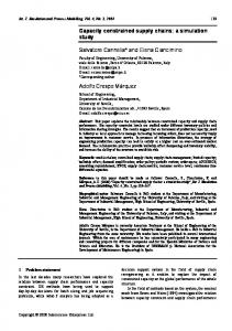
Dial then explains that standard shortest path algorithms have to be adapted for the transit case because the Markov property is violated. The Markov property states that the route choice probabilities at a node are independent of the travellers’ origin. Further, in the example of Figure 3-1 passengers destined for C will take longer to get to B than passengers destined for D if Line II is more frequent. Dial therefore
28
adapts Moore’s shortest path algorithm (Moore, 1957). The adapted algorithm stores the waiting time for the transfer to the trunkline the route is using. If there is a through service at the trunkline exit the current waiting time is subtracted but a (larger) waiting time for the through service is added.
A
Ι, ΙΙ
Ι
C
ΙΙ
D
B
Figure 3-1 Simple transit network with Trunkline between nodes A and B. A major critique of Dial’s work is that this algorithm can not deal with the situation where lines connect the same OD pair but have different travel times. In the example of Figure 3-2 Dial’s algorithm would assign all passengers to Line II for the journey between A and B and passengers destined for C would change at B.
A
ΙΙ Ι
Ι
C
ΙΙ
D
B
Figure 3-2 Simple network with a fast (Line II) and a slow (Line I) service between A and B. Fearnside and Drapper (1971) also based transit assignment on a road-assignment tool. In their model each node is represented by line specific nodes and boarding and alighting links. For example, node B as shown in above figures is represented as in Figure 3-3. An advantage is that this network representation allows the inclusion of waiting times and line specific transfer penalties which might reflect longer walking ways to node BII compared to node BI. The model was further developed in order to
29
be used in multi-modal studies. The disadvantage of this representation is the multiplicity of links and nodes, which Dial attempted to avoid.
A
Ι
BΙ
Ι Boarding
BC
A
ΙΙ
Alighting
BΙΙ
ΙΙ
Figure 3-3 Interchange at Node B in Fearnside & Drapper (1971) network
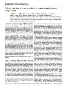
Fearnside and Drapper assume that passengers have to decide for node BI or BII before boarding. This leads to an overestimation of waiting time if it is realistic to assume that passengers choose the first vehicle arriving from several possible (“common”) lines. As explained in the introduction transit networks with fast and slow lines (as in Figure 3-2) are good illustrations of the common line problem, where passengers include more than one route in their choice to minimise the travel time: In Figure 3-2 passengers for C might consider taking Line I as well as Line II from A. Especially if a passenger has just missed Line I, he/she will consider taking Line II to B in order to catch up with the slower Line I at this node.
The first papers on the common line problem “fixed” the routes of the passengers by calculating the shortest path to the destination according to link travel times and expected waiting times, which are reduced if several lines serve this path. Le Clerq (1972) developed an algorithm that searches for the shortest paths by looking at all possible interchanges from the service the traveller is currently using. The link travel
30
times and waiting times for each interchange are considered in the cost function. The algorithm therefore takes account of the fact that the Markov property is not holding for transit networks and also allows for different travel times of different services. In the example of Figure 3-2 the route choice will however still be fixed. Passengers destined to C will always take Line I if the expected average waiting time for interchange at B is larger than the additional on-board travel time for Line I. Similarly, if the waiting time at B is smaller then all passengers destined to C will take Line II and interchange at B.
3.2.2. Route-section and strategy-based approaches
Spiess and Florian (1989) showed, however, that passengers can often significantly reduce their travel time when they consider several paths to their destination. Following Lampkins and Saalman (1967), who explained that passengers will exclude lines from their choice set if they are obviously bad, e.g. travel time of slow line is longer than travel time plus headway on the fast line, Spiess and Florian explained that passengers develop so-called strategies if more than one transit line leads to their destination from their current location. In this case, passengers predetermine a set of attractive routes among the routes that bring them to their destination (possibly via very different paths) and choose the first vehicle arriving from this set of attractive lines. Therefore in fact not the traveller but the vehicle arriving first (from the set of attractive lines selected by the passenger) decides the route the traveller is taking. In the example of Figure 3-2, the passenger destined for C will minimise the travel time by choosing Line I or Line II at A whichever vehicle is arriving first. This is if the travel time for I is not larger than the travel time plus
31
the expected waiting time for Line II, otherwise the optimal strategy is to always wait for Line II.
Nguyen and Pallottino (1988) illustrated this problem by introducing the term hyperpath. A hyperpath consists of a set of paths that are potentially taken by the user depending on the arrival of the first vehicle at the passenger’s origin and the stations where he or she has to interchange. The probabilities of taking a path are given according to the line frequencies, so the problem is reduced to finding the shortest hyperpath, i.e. the set of paths that should be included in the traveller’s route choice. The underlying behavioural assumption is: “Before starting any trip, a passenger has chosen a fixed subset of transit lines for every stop he may encounter on his trip, and for every transit line the alighting point.” (Nguyen and Pallottino, 1988). The authors note that the sequential procedures by Dial (1971) are similar; however, the hyperpath concept does not suffer from “independence of irrelevant alternatives” disadvantage that besets logit assignment. The hyperpath model leads to the same solution as Spiess and Florian’s model, but with a more flexible network description that allows for more efficient computational techniques on larger networks. Cominetti and Correa (2001) for example use the hyperpath concept to adapt Dijkstra’s shortest-path algorithm to a “shortest hyperpath algorithm”.
The main challenge in the strategy approach is to find the set of routes S that minimises the expected travel time Ts, which is given by (3.2): Ts = E (Ws ) + ∑ t i H i ( S )
(3-2)
i∈S
32
where E(Ws) is the expected waiting time, ti the expected travel time and Hi(S) the probability that route i is served first. Chiriqui and Robillard (1975) suggest a heuristic algorithm to solve this problem. Their algorithm is based on ordering the routes according to their in-vehicle travel time in ascending order. Ts is first calculated taking the route section with lowest ti only. If adding other route sections reduces Ts then these are added. If adding a route does not reduce Ts further, the algorithm stops. The motivation behind this algorithm is that it is illogical for a passenger to let a bus of a given route go by and wait for a bus with longer in-vehicle travel time. It is obvious that this heuristic has its limit in large scale networks where the enumeration of all routes becomes difficult.
Chiriqui and Robillard (1975) and De Cea and Fernández (1993) use a model with dual network representation, also referred to as “route segments” model (Figure 3-4). The idea is that each stop that can be reached without interchange is represented as a separate link, a so-called “route section”. Therefore waiting times will only have to be considered at the boarding node of a “route-section”.
S2(Ι)
A
S1(Ι, ΙΙ)
S4(Ι)
C
B S5(ΙΙ) S3(ΙΙ)
D
Figure 3-4 Simple transit network with route sections (dual network)
33
A route section can also include several lines with different travel times as shown in Figure 3-4 with S1. In this case the expected in-vehicle travel time is calculated in proportion to the frequency of each line as in (3.3).
tS =
∑f t j∈S
j j
∑f i∈S
(3-3) i
Because Chiriqui and Robilliard (1975) and De Cea and Fernandez (1993) do not explicitly use strategies this leads in general to a suboptimal solution. The slightly larger example network used by Spiess and Florian (1989), as well as De Cea and Fernandez (1993), illustrate this well (Figure 3-5 and Table 3-1). In the route section model passengers will choose the section that minimises the costs (and it is not considered that other routes might be quicker if they arrive earlier). Within the lines of a route section the flow is assigned to the specific lines according to their frequency. In Figure 3-5 this leads to S1 not being used, whereas Spiess and Florian show that the optimal strategy includes using Line 1. Line 1 is for example quicker if it arrives immediately and passengers experience the expected waiting times for Lines 2 and 3. In general the approach using explicit strategies will lead to greater route dispersion.
34
L1(25min, 10/hour) L2(7, 10)
A
B
L2(6, 10) L3(4, 4)
C
L3(4, 4)
D
L4(10, 20) a) Spiess and Florian (1989) example network
S1 (L1) S5 (L2) S2(L2)
A
B
S3(L2,L3)
C
S4(L3,L4)
D
S6 (L3) b) Same network with route sections Figure 3-5 Example network used in Spiess and Florian (1989) and De Cea and Fernandez (1993)
Table 3-1 Differences in assignment results for network in Figure 3-5 Link usage
Early work
Dial (1967); Fearnside and Drapper (1972)
v1 v2 (A-B) v2(B-C) v3(B-C) v3(C-D) v4
1 0 0 0 0 0
Route Sections model (Chiriqui, 1975; De Cea and Fernandez, 1993)
Strategy model (Spiess and Florian, 1989)
0 1 0.83
0.5 0.5 0.5 0 0.08 0.42
0.17 0.83
Chiriqui and Robillard (1975) point out that the “clever” passenger will reduce his travel time by observing the time he had to wait for the vehicle arriving first. If taking this vehicle means that his travel time is larger than the expected travel time
35
he might wait for a faster service on the basis that it is likely to arrive soon. This assumes an exponentially distributed waiting time with mean being the headway. If the arrival process is irregular this is of course not the case.
In general, the strategy will be more complex, the more information the passenger has and the more opportunities the network offers. Three levels of information and strategy complexity can be distinguished: If the passenger is bound to a specific line (e.g. because of ticket restrictions) he or she fixes the route before arriving at the platform (Level 1). The traveller might buy his or her ticket and make the route decision on the assumption that he or she has perfect information about the best route to his or her destination.
If, however, the passenger does not have to make the route decision before arriving at the platform, the route choice might be governed by the next vehicle arriving, e.g. several lines offering a service to the passenger’s destination or at least closer to the destination (Level 2). This is the common line problem as considered in the Spiess and Florian (1989) paper and the case most literature deals with. The passenger only knows the frequency of the services (and not the exact remaining waiting time until the arrival of the fast vehicle) and if the traveller sees the slower service arriving, he or she might prefer to take this vehicle, because the expected waiting time for the express service is too high to make it worthwhile waiting.
Nowadays, the passenger often has information about the arrival times of the subsequent vehicles as well. This third level of information is realistic for transit networks, where passengers can buy a network ticket and displays on the platforms
36
show the sequence and time left for the next trains arriving (metros and some buses in the U.K.). In this case the traveller might for example skip the next vehicle arriving, because he or she knows that an express-service is waiting to enter the station.
3.2.3. Linear Programming formulation and solution
algorithm to the common line problem In Spiess and Florian (1989) every route is represented with a link between each stop with the attributes travel time and frequency. Boarding links have no travel time but a frequency associated with them, alighting links have a cost of zero travel time and zero frequency.
With the assumption of exponentially distributed interarrival times the expected waiting time for each link can be calculated as in (3.4) with the sum of the frequency f of all attractive outgoing links A+ at a node i, and the link probability Pa as in (3.5) with the frequency of this line compared to the frequency of all attractive lines at this node. W ( Ai+ ) =
1
∑f
a∈Ai+
Pa ( A i+ ) =
(3-4) a
fa
∑
a∈ Ai+
fa
(3-5)
A non-trivial task is to find the optimal strategy that reduces the total journey time. Spiess and Florian present the problem as a linear program. The objective is to find the strategy that minimises the sum of the expected total travel time including waiting time for all flow from all origins to a destination. For each destination the 37
problem is formulated as in Eq. 3.6 where va is the flow of link a, and wi is the total expected waiting time at node i. Min ∑ c a v a + ∑ wi a∈ A
(3.6)
i∈I
The constraints belonging to the objective function (3.6) are firstly, flow conversation at each node, secondly the relationship between link flow and frequency stemming from the assumption that passengers board all attractive lines in proportion to their normal frequency (3.5) and thirdly the non-negativity of link flows.
Finally, they construct the dual formulation of the problem. The minimisation problem becomes a maximisation problem and the Lagrange multipliers ui can be interpreted as the expected total travel time from node i to the destination but excluding the waiting time at i. The formulation of the dual problem is also the basis for the solution algorithm. The algorithm is composed of two steps; in the first the optimal strategy is found and in the second the traffic is assigned from all origins to the destination. The algorithm needs to be solved for each destination separately. It searches from the destination to all origins by taking the links closest to the destination first with increasing order. The key to finding the optimal strategy is then a comparison of the costs ui and uj +ca for each link from i to j. If uj +ca ≤ ui the link a will be added to the attractive links at node i. Since this comparison does not include the waiting time, this means that if the route arrives first at i, this service will be a shorter route than all options looked at so far. If the above comparison holds, the service frequency for the node will be increased by the frequency of the newly added service. This search for the optimal set of arcs is the same as the search for the
38
optimal hyperpath in the graph theoretic interpretation of the problem by Nguyen and Pallentino (1988).
Spiess and Florian prove that the solution obtained by the algorithm is an optimal one by a) showing that (u*, v*) are a feasible solution for the primal and dual problem and b) that the complementary slackness conditions are fulfilled. These state that for all used arcs the constraints of the primary problem are strict equalities. Optimality follows then directly from the linear programming theorem.
De Cea et al (1988) present a mathematical formulation of the route sections model as in Figure 3-5b which is very similar to above formulation. The dual variables in the model have the same meaning and the solution algorithm also follows an adaptation of Dijkstra’s shortest path algorithm. De Cea et al further explore the differences between results produced by the “strategy” and the “route section” model. Both approaches are tested on a large scale network with a high percentage of links that carry common lines. The results confirm those shown in the previous section, where the strategy approach leads to a wider and more equal distribution of flows on more routes. However, De Cea et al conclude that the differences in flows are not large but that the route section approach requires a significantly longer computation time. In reality the difference between the approaches will depend on factors like the fare scheme. If passengers have to pay each time they board there will be almost no difference but if there is one fare for the whole network the differences are likely to be larger since the route section approach will underestimate the route dispersion.
39
3.3.
The effective frequency approach 3.3.1. Problem description
Spiess and Florian (1989) discuss the extension of their model to the case when link costs are depending on link flows, i.e. ca(v). This could be used to model discomfort in crowded vehicles. In this case their proposed solution algorithm needs to be adjusted since the problem can not be solved destination by destination. The linear problem can be restated as a convex optimisation problem which is then solved with the linear approximation method. The method requires that the cost function must be continuously monotone increasing, which is not necessarily the case. A second limitation of this approach is that all passengers on board the vehicle suffer the same inconvenience, independent of where they boarded. This assumption neglects the fact that passengers boarding earlier are more likely to get a seat and therefore are less likely to experience inconvenience through crowding. A third limitation with this approach is that it assumes that the service frequencies are not affected by crowding.
Similarly, Lam et al (1999) propose to solve transit assignment with capacity problems through the introduction of “line specific overload delays”. The problem with their approach is also that it does not consider priority rules on transit systems. Passengers already on-board will not be deterred by passengers attempting to board later. The achievement of the Lam et al paper is rather that it formulates transit assignment as a stochastic user equilibrium problem. The problem is formulated as a mathematical programming problem and the Lagrangian multipliers of their solution are equivalent to the line specific overload delays. In Lam et al (1999) the frequency of the transit line is fixed, in Lam et al (2002) this is relaxed through the assumption
40
that the number of passengers boarding and alighting will influence the dwell time and hence the service frequency. However, in summary, flow dependent link costs are only suitable to model on-board inconvenience but not to model the problem of limited capacity.
3.3.2. Effective frequencies with practical capacities
Spiess and Florian mention that the aforementioned limitations can be overcome with the “effective frequency approach”. This approach is followed up by De Cea and Fernández (1993). The travel costs of transit arcs are assumed to be constant but the travel costs of waiting links are dependent on the link flows. Since the De Cea and Fernandez model is based on route sections there is a waiting link for each route section link. This one-to-one relationship makes it possible to collapse waiting links and transit links into a single link with in-vehicle cost plus waiting cost. The waiting cost term consists of two parts where the second term is a function of the route ~ section flows Vs , the flow on other route sections competing with this flow Vs ,and
the “practical capacity” K s of this link (3.6). The in-vehicle cost t s is calculated with Eq. (3.3).
~ ⎛ Vs + Vs cs = t s + + βϕ s ⎜⎜ fs ⎝ Ks
α
~ ⎛ Vs ⎜ w = + ϕ⎜ fl ⎝ Ks i l
α
⎞ ⎟ ⎟ ⎠
⎞ ⎟ ⎟ ⎠
(3-6)
(3-7)
The condition on the flow function ϕ s is that it needs to ensure that cs is strictly monotone increasing with Vs. De Cea and Fernández suggest a power function with n
41
between 4 and 6 based on the experience for car networks. They note that Ks is not a real capacity but that “as n increases, Ks acts more and more like a real capacity”. It is important to note that this approach does not guarantee that lines will not be ~ overloaded. The competing passengers Vs are made up of those passengers using all
other route sections that contain lines that are part of section s and alight after node i(s), the origin of route section s.
The effective frequency is then defined as the inverse of the waiting time index wli (3.7). The idea behind this is that with more buses arriving full, the waiting time will increase, because it is harder to get onto the vehicle. If the vehicle arrives empty the effective frequency at node i, fli, is equal to the nominal frequency fl. On the other side a service will never be totally full because with increasing congestion fli → 0, but fli = 0 will never be reached. De Cea and Fernández define the effective frequency as being the same for all passengers waiting. It is not considered that a high number of passengers wishing to board will reduce the chance for an individual to board.
De Cea and Fernández prove that the set of attractive lines monotonically increases with congestion and that the set of attractive lines in uncongested situations is also among the attractive lines in congested situations. Further, with this definition of effective frequency and wli dependent on the link flows the equilibrium problem is no longer linear. De Cea and Fernández conclude by presenting two algorithms to find an equilibrium solution that satisfies Wardrop’s principle (which states that the costs on all used paths is equal to the minimum cost and the flows on all paths with costs greater than the minimum cost is zero). In the first algorithm, congestion is only
42
considered at the route section level. The line frequencies are assumed to be constant ~ but the costs still depend on the ratio ( Vs + Vs )/ K s . This means that the user
equilibrium condition has now an equivalent convex cost optimisation problem that can be solved with a Frank-Wolfe-type-algorithm. In this algorithm one calculates the minimum cost routes along the search direction
∂c and assigns the demand to ∂V
the newly obtained routes. If two subsequent iterations produce sufficiently close solutions the stopping criterion is fulfilled.
The second algorithm does assume effective frequencies before using the FrankWolfe type algorithm but loads the lines sequentially starting with the depot where it is known that the effective frequency equals the nominal frequency. Once the lines have been loaded
∂c can be built and an improved solution can be found. This ∂V
method is computational very demanding and De Cea and Fernández further do not give a formal proof of convergence for this intuitively correct solution method.
Both solution methods are demonstrated with the example network shown in Figure 3-5. In Chapter 3.2 the solution to the uncongested problem has already been presented. Results with the linearised approach show that if the network becomes mildly congested S1 becomes additionally attractive. In case of extreme congestion also route A→S2→B→S6→D is used. Line 1 is heavily overloaded in case of extreme congestion. Using the exact algorithm only leads to a slight reduction of the overloading on Line 1.
43
3.3.3. Effective frequencies with strict capacities
De Cea and Fernández (1993) acknowledge that “practical capacities” do not solve the problem of overcrowding. According to De Cea and Fernández, strict capacities will further not allow for explicit performance and convergence functions. However, they argue that this approach might be sufficient for strategic planning where one is not concerned about passenger loads for specific runs but is looking at the demand for the service over a longer time period.
Cominetti and Correa (2001) point out further shortcomings of the De Cea and Fernández approach. In particular they show that the above approach does not guarantee that Wardrop’s first principle is fulfilled. Cominetti and Correa prove that in some congested situations, costs can be minimised by a split between two strategies. Consider a network with one OD pair and two direct services between these where t1 < t2 . The strategy to consider Line 2 only is obviously not optimal. Therefore passengers at the origin have the choice between two strategies: The first one is to wait for Line 1 and the second strategy is to take whichever line arrives first.
If the waiting time is not very high compared to the in-travel time in uncongested situations it is clearly better to wait for Line 1 even if Line 2 arrives first. Applying Spiess and Florian (1989) or De Cea and Fernández (1993) would yield the same result. In highly congested situations, the effective frequency approach of De Cea and Fernández would predict that it is better to use Strategy 2 because the effective frequency is much reduced compared to the nominal frequency (or in other words: “Since the network is congested and the fast service might be full, do not rely on this service but take whichever service is arriving first”). Cominetti and Correa (2001) 44
point out that it can however be easily shown that for certain demand regions a strategy mix in fact would reduce overall travel time. If in highly congested situations some passengers stick to Strategy 1 this would reduce overall travel time. In reality it might not be realistic to assume that some passengers would stick to Line 1 and not consider boarding Line 2, but this theoretical result shows that if in highly congested situations the operator would reduce the choice of some passengers, this can improve the overall performance of the network.
Cominetti and Correa (2001) then describe some conditions for this area of flow where a strategy-mix between two strategies is optimal. They further show that there are some areas where a flow increase does not result in an increase in travel cost as the demand can be accommodated by an uncongested line without cost increase.
Cominetti and Correa further use a formulation of the effective frequency based on queuing theory: If vi → vi then fi’ → 0 and wi → ∞ where vi is the saturation flow and wi is the waiting time on the link. With this formulation of “strict capacities”, line loads will not exceed capacity. A further improvement of this paper is that they simplify Spiess and Florian’s formulation by using only arc flows and not strategy flows. Therefore it is not necessary to keep track of the different origins in the assignment. The assignment algorithm assumes that passengers travel on shortest hyperpaths and Dijkstra’s algorithm is used for finding shortest hyperpaths. As in De Cea and Fernández, the distribution of flows across links of a hyperpath is proportional to the effective frequency of this link.
45
Cepeda et al (2006) continue the work of Cominetti and Correa (2001) and prove some important characteristics of transit assignment with effective frequencies. Firstly they show that the ratio va / fa can be assumed to be an (unknown) variable and is not a constant that needs to be determined before calculating the network equilibrium. This allows applying the Cominetti and Correa (2001) approach for large scale networks. Secondly, they show that the global equilibrium is not trapped by a local equilibrium. Therefore it is possible to use a gap function that becomes zero if the solution is equal to the optimal one. The gap function is based on Wardrop’s first principle and shows the difference between the cost of all passengers using the cheapest hyperpath and the cost for all passengers with the current assignment. Based on these findings they propose a heuristic solution algorithm using the Method of Successive Averages that solves congested transit assignment for large-scale networks. Several case studies in major cities around the world are briefly described demonstrating the validity of this approach.
3.4.
Approach with fail-to-board probabilities
One of the earliest models to take into account capacity constraints is the TRANSEPT model presented by Last & Leak (1976). The purpose of the model was to predict patronage on bus routes. Several case studies were conducted in complex networks and robust results achieved. The model is used in multi-modal studies estimating the mode choice between walking, car and bus with a logit model. It can be applied in order to evaluate the cost benefits for users and operators for different allocations of the buses.
46
In their model they use an intermediate level of network representation for bus routes to take advantage of the fact that many bus services use the same paths for large sections of their routes. Sections of routes where no bus routes start, end or divert are represented as one link. Interchanging between different bus routes is only possible at the end of such a link. TRANSEPT further assumes that all passengers take the shortest path, which means that the common line problem is not taken into account in so far as the choice of path might also depend on which vehicle is arriving first.
The choice between specific bus routes (on a common line) takes waiting times as well as capacity constraints into account. The headway is calculated as the sum of the frequencies and the average waiting time is calibrated with survey data. A logit model is used to distribute the demand between the routes according to their attractiveness and capacity constraints are then taken into account within an iterative process. The competition for space is modelled by loading the services from upstream to downstream. In this way the priority of those boarding further upstream is observed. This procedure allows calculating a probability of failure-to-board for each route and stop. This failure probability is used to increase the average waiting time. An iterative process is then used to load the network and “stabilise” the waiting times. Probability distributions are used to estimate the number of passengers boarding as well as alighting at each stop. The model requires that the overall capacity is sufficient for the demand as the waiting time would otherwise grow to infinity. If this is not the case, the model allocates additional buses to critical routes.
47
Last and Leek (1976) do not describe the mathematical formulation of their model in detail, so that it is not fully clear how they stabilise the waiting times. It is however clear that their procedure of “Looking for a stable solution” is not always realistic. Let us assume that the example network used before has the demand and capacity constraints as shown in Figure 3-6. In this case, the only stable solution would be if all passengers destined for C would take Line I at A. As explained before, this might however not be the case, because Line II will be more attractive to passengers for C if it arrives first. De Cea and Fernández (1993) further point out that loading the TRANSEPT network link by link means it is only feasible for radial networks. Demand AÆC: 100; AÆD: 100 Capacity Line Ι and ΙΙ: 100
A
ΙΙ
Ι
C
ΙΙ
D
B
Ι
Figure 3-6 Transit network with capacity constraints
3.5.
Passenger distribution between different paths of one hyperpath (bus stop problem)
Bouzaïene-Ayari et al (2001) point out that in the previous literature the distribution of passengers between the attractive lines of a strategy/hyperpath at a node is not always realistic. Instead of a priori using the nominal or effective frequency as basis for the distribution, Bouzaïene-Ayari et al generalise Eq. (3.5) and use formulation
48
(3.8) where ξa is the so-called attraction factor for arc a which is included in the set of attractive lines A+ at node i.
P ( A i+ ) =
ζa ∑ζa
(3-8)
a∈ Ai+
Instead of using ξa = fa (Spiess and Florian, 1989; De Cea and Fernández, 1993) or
ξa = fa’ (Cominetti and Correa, 2001) Bouzaïene-Ayari (1988) showed with a simulation of several bus stops that in heavily congested situation ξa = (1-va)fa/Ka is a better approximation.
Bouzaïene-Ayari et al however point out several shortcomings of all these models. First of all ξa = fa obviously does not allow for the possibility that one might not be able to board a vehicle because of overcrowding. Secondly, all above functions for ξa assume that all transit lines have the same exponential distribution of waiting time. This implies high service irregularity for all attractive lines. This might however not be true and it should be considered that the regularity between the services might differ. At a node where passengers can board trams as well as buses, the trams might well be significantly more regular. To overcome this problem, Gendreau (1984) and Bouzaïene-Ayari et al propose to use an Erlang distribution for the waiting time of each line with a line specific shape parameter k. They state that the Erlang distribution has a number of well known properties which are widely used in queuing theory. Further, with k→1 an extremely irregular distribution and with k→∞ a deterministic distribution of the line regularity can be modelled.
49
Finally, Bouzaïene-Ayari et al describe that the models considering congestion,
ξa(va), are not necessarily consistent with the theory of strategies. If there is a mix of strategies, i.e. some passengers will always wait for the fast service, whereas others will take whichever service arrives first, then a model ξa(va) might predict a higher waiting time for the latter strategy. They state that this is however irrational. The effective frequency approach leads to this because flow increases travel time even if flow is lower than capacity. Bouzaïene-Ayari et al’s critique of this being irrational is not justified if one considers inconvenience costs for travelling with the more crowded line: The passenger with the strategy “take whichever line comes first” might well encounter higher costs because less waiting time is outweighed by onboard vehicle crowding.
In order to overcome these shortcomings, Bouzaïene-Ayari et al propose that ξa = 1/ Wa(va) where Wa is the waiting time function for line a. Different waiting time
distributions can be assumed where one needs to consider that those with strict capacity constraints (Wa → ∞ for va → v a ) are more difficult to integrate into assignment models than those with practical capacity constraints (Wa → ∞ for va →∞).
In general it can be concluded that Bouzaïene-Ayari et al’s work defines waiting time more accurately if good data are available. It is important to note that the work of Bouzaïene-Ayari only concerns the distribution of passengers at a bus stop. The paper does not consider the problem of finding the optimal set of links that should be included in the strategy/hyperpath.
50
3.6.
Discussion
This chapter reviewed the major approaches to frequency-based transit assignment. It was first shown that the first assignment approaches, which were based on traffic assignment assumptions, did not consider that the Markov assumption does not hold for transit assignment. Passenger route choice at any given interchange will depend on the destination as well as the origin. Further improvements to frequency-based transit assignment did consider the common line problem. Chapter 2 discusses in which situations the common line problem is applicable and that passengers develop different strategies depending on the information about train arrival times. A solution to transit assignment with common lines based on linear programming is discussed following Spiess and Florian (1989).
The second part of this chapter reviews assignment that considers the consequences of capacity shortages. The most frequently used approach is the “effective frequency” one. Approaches with practical and with strict capacities have to be distinguished. Using practical capacities means that line-overloading is still possible. It further leads to situations where the Pareto-optimal solution is not equal to the network equilibrium. There are problems to find an equilibrium with the strict capacity approach as the network capacity might actually not be sufficient. Cepeda et al (2006) suggest using a dummy network that connects all destinations with walking
links. Cominetti and Correa (2001) show that the problem can be described as a fixed point problem. But so far only heuristics are developed for the case where one allows
51
for the effective frequency influencing the route choice of passengers. Nevertheless, the approach has been shown to successfully model large scale overcrowded networks.
The effective frequency approach assumes strictly increasing cost functions for increasing demand. This can reflect discomfort caused by congestion. It does however not accurately reflect the cost of missing a vehicle due to overcrowding. The cost for this will increase rather more like a step function. One could however argue that, in heavily congested situations, a continuous function reflects the continuously increasing probability of missing a vehicle due to overcrowding. However, assuming that this risk of failing to board (an additional cost in heavily congested situations) is a continuous and not a different function from the discomfort caused through full vehicles is a major assumption. A further critique of the effective frequency approach is that it does not allow estimation of the number of passengers that are not able to board the vehicle. It is therefore also not suitable to model the build-up of congestion over time.
Chapter 2 reviewed schedule-based assignment approaches and in particular dynamic capacity constraint models. As mentioned in Chapter 3.3 De Cea and Fernández (1993) argue that for strategic planning one is not interested in passenger loads for specific runs. This is true for frequency-based services but one might still be interested in dynamic effects. For example providing sufficient capacity for the demand of the extended morning peak might still lead to severe congestion during the peak of the peak. Overcrowding within short time intervals are safety risks for the
52
whole service and lead to delays and hence reduced overall capacity during long periods of time.
In the following chapters an alternative to the effective frequency approach is described which is aimed at overcoming some of its shortcomings.
53
4.
Using Absorbing Markov Chains in Transit
Assignment: The CapCon Model
4.1.
Introduction
The literature review highlighted several shortcomings of frequency-based assignment. Especially in congested situations when the demand might exceed the network capacity, and when the demand is changing over the assignment period the weaknesses of the currently available transit assignment tools are known. To overcome some of these shortcomings the following new method is developed. A main feature of this model is the explicit inclusion of strict capacity constraints, which is why the model is referred to as “CapCon”. These capacities are line specific and the approach does not rely on effective frequencies. This approach allows an explicit estimation of the number of passengers not being able to board which is also the basis for the dynamic extension described in Chapter 5.
This chapter first explains the network description and the notation used throughout this and the following chapters (4.2). Then the cost elements that are considered for the path choice are described, in particular the “risk of failing to board because of overcrowding”. In 4.3 it is explained how this cost can be described node specifically, which is the requirement for the optimal hyperpath search algorithm in 4.4. Chapter 4.5 explains how the path choice probabilities are used to calculate the network equilibrium and in 4.6 it is shown that there is a unique equilibrium for non-circular
54
as well as circular lines if one assumes passenger mingling. The network loading procedure becomes a deterministic user equilibrium assignment with the application of the MSA described in Chapter 4.7. If one does not consider common lines the hyperpath search becomes the search for the shortest path and also the network description can be significantly simplified. This is described in Chapter 4.8.
Sections 4.9 and 4.10 conclude this chapter. In Section 4.9 an application of the CapCon model to a small example network is described. The effects of introducing common lines and passenger risk averseness are shown. Finally, Section 4.10 gives a short summary and discusses the merits and shortcomings of this approach. The model presented in this chapter has also been published in several publications: Bell et al (2002) discuss the idea of applying absorbing Markov chains to network analysis and transit assignment, Schmöcker and Bell (2004) introduce capacity constrained transit assignment and Kurauchi et al (2003) focus on the path choice algorithm by replacing it with a search for the optimal hyperpath.
4.2.
Network description and its notation 4.2.1. Network representation
Figure 4-1 shows the nodes and arcs of a station which has one platform and which is served by one line only. Besides the origin and the destination there are five node types. The stop node represents the bus stop or platform at which passengers wait for the service to arrive. To consider the capacity constraints failure nodes are introduced. The section on network loading will describe that all demand exceeding
55
the available capacity is not transferred further to the boarding node but instead to a fictional “bin” or excess demand node. It is further important to note that the network loading procedure assumes that at the boarding node passengers who board the service at this station and those who boarded upstream and did not alight mingle. At the alighting node passengers who stay on-board and those who alight at this station are separated, so that at the stop node alighting passengers, passengers who start their journey at this station and those passengers who failed to board at this stop node in the previous time interval mingle.
There are nine arc types which connect the nodes described above. Line arcs correspond to transit lines and connect a boarding node with the alighting node of the next station downstream. The cost of travelling on a line arc is assumed to be equal to the travel time between these two stations on this line. On-board wait arcs are used by passengers not alighting at this station. The cost of these arcs is equal to the dwelling time of the service at this stop. Access-walking arcs and egress-walking arcs connect the origin with the stop node and the stop node with the destination
respectively. There is exactly one access arc and one egress arc in every hyperpath. The cost of walking from the origin to the first platform and the cost of walking from the last destination is currently not considered. Also alighting arcs, which connect alighting and stop nodes, and boarding-demand arcs, which connect a stop node with a fail node, do not have a cost associated with them. In order to reflect the reduced waiting time if passengers include common lines the waiting time is not associated with the boarding-demand arc or the boarding arc but instead with the stop node. For those passengers who get on the service, i.e. do not fail at the failure node, there is no additional cost, meaning that there is no cost associated with boarding arcs. The
56
amount of passengers exceeding the available capacity is transferred to their destination via the failure arcs. Note that they are transferred to their respective destination via the same failure arc, as the destination of the failure arc is redirected to the destination of the passenger at the beginning of each hyperpath search as explained in Section 4.4. This allows the formulation of the model in terms of flow conservation, i.e. all demand is reaching its destination: Passengers who do not fail to board anywhere without usage of failure arcs and those passengers who do fail to board with the usage of exactly one failure link. Figure 4-1 illustrates that the excess demand is removed from the downstream nodes. The cost of a failure arc is assumed to be related to the passenger’s fear of failing to board and the probability of failing to board which is discussed in Section 4.3. On-Board Wait
O Ac ce ss
Alight
Alight
Eg
re ss
Line
D
Stop
Boarddemand
Fail
Boarding
Board
Line
Fai lur e Dest. of excess demand
Figure 4-1 Network representation of a station with 1 platform and 1 transit line
Figure 4-2 shows the arcs and nodes needed to represent a station with multiple platforms and lines. It is important to note that failure nodes, alighting nodes and boarding nodes (and hence also the arcs leading into or out of these nodes) are
57
transit line specific. However in general stop nodes are not line specific as there is for each platform or bus stop only one stop node. The figure further illustrates that the stop nodes belonging to the same station are connected via transfer arcs. There is one transfer arc connecting Platform 1 with Platform 2 and a second transfer arc representing walking in the opposite direction. The cost of the transfer arcs is set equal to the walking time between the two platforms.
Platform 2
s es c Ac
Eg res s
Ac c
Line
es
D
Transfer
O
E
s
On-B oard
Alight Alig h
t
Stop g Ali
Line
Alight
ss gre
ht
Fail gn i ard d Bo man de
Boarding
Board
Line
Excess Demand
B de oar m din an g d -
Fail
Wait
Boarding
W oard On-B
Board
Line
ait
Platform 1
Figure 4-2 Station with 2 platforms and 2 lines serving platform 1
58
4.2.2. Notation (Glossary)
For the mathematical formulation of the assignment model the following notation will be used throughout this thesis. Four groups of variables can be distinguished: Global, node-specific, arc-specific and hyperpath-specific variables. Global
n:
Number of nodes in network
no:
Number of origins o in network
L:
Set of Transit Lines (with l ∈ L and Lu: Set of transit lines served at platform u)
capl:
Capacity of a service on line l
R:
Set of stations (with r ∈ R)
Ul:
Set of platforms served by line l (with u ∈ U)
θe:
Sensitivity to boarding overcrowded services (risk averseness)
Nodes
I:
Set of Nodes (with i ∈ I)
Out(a):
The node arc a is leading out of
In(a):
The node arc a is leading into.
E:
Set of failure nodes (with e ∈ E and eul denoting a failure node associated with platform u and line l)
η i:
1 if node i is a failure node and 0 otherwise
S:
Set of stop nodes (with s ∈ S and su denoting a stop node at platform u)
σ i:
1 if node i is a stop node and 0 otherwise
B:
Set of boarding nodes (with b ∈ B)
qi:
Failure probability at node i
spai:
Available spaces at node i (vacancies for passengers wishing to board)
spri:
Remaining spaces at node i (remaining vacancies after all passengers boarded)
yd:
Vector of demand from origins o to destination d
v:
Passenger flow vector travelling via nodes i (vd: and destined for d)
59
Πd :
Matrix of transition probabilities from node i when destined for d
Θ d:
Matrix of transition probabilities to an intermediate node j
δ:
Vector of transition probabilities from node i to destination d
Arcs
A:
Set of Arcs (with a ∈ A)
x:
Passenger flow vector travelling via arc a (xd : destined for d)
waitul:
On-board waiting arc on platform u for passengers staying on line l
lineul:
Line arc out of platform u on line l
board-dul: Boarding demand arc on platform u for line l boardul:
Boarding arc on platform u for line l (The adjusted arc-flow considering capacity constraints)
on-boardul: On-board wait arc on platform u for line l ca :
Cost of travelling on arc a connecting nodes i and j
fa :
Frequency of transit service on arc a. Note that fl and fl(a) are also used because fa is usually (but not necessarily)constant for all arcs served by the same line l
πah:
Arc split probabilities. (Probability to choose arc a when traveller is at Out(a) and travelling on hyperpath h)
Hyperpath specific
Hd:
Set of all feasible hyperpaths to destination d (with h ∈ Hd)
hi:
Hyperpath connecting intermediate node i to destination d
zh :
Flow on hyperpath h in the set of used hyperpaths
Ih :
Set of nodes within hyperpath h
Sh:
Set of stop nodes within hyperpath h
Eh:
Set of failure nodes within hyperpath h
Ah:
Set of arcs within hyperpath h (Ahi: Subset of arcs leading out of node i)
gh:
Cost of travelling hyperpath h
wih:
Expected waiting time at node i when travelling on hyperpath h
αah:
Probability of using arc a when travelling on hyperpath h
60
βih:
Probability of traversing node i when travelling on hyperpath h
Ph:
Set of elementary paths within hyperpath h (with p ∈ Ph)
εip:
1 if node i is element of path p, 0 otherwise
δap:
1 if arc a is element of path p, 0 otherwise
λp:
Probability to choose elementary path p
4.3.
The cost of a hyperpath
4.3.1. Elementary paths and hyperpaths
In Chapter 3 the common lines problem is explained. Common lines are respected in the following approach: It is assumed that the passengers select a set of lines from which they choose the first service arriving. Therefore, they are not choosing a shortest path p, but a set of a paths that minimises the travel time or generalised costs. As explained in Chapter 3, following Nguyen and Pallottino (1988) this set of attractive paths Ph is called Hyperpath H and the set of paths that minimises the travel costs needs to be found. The following describes how the cost of such a hyperpath can be calculated. Note that the cost of a hyperpath is always equal or lower to the cost of any elementary path p ∈ H connecting origin o and destination d.
4.3.2. Transition probabilities
In order to search for the shortest hyperpath the arc transition probabilities need to be defined. For every node i the arc transition probabilities πah satisfy:
∑π
a∈ Ahi
ah
= 1 , ∀i ∈ I h
(4-1)
61
In (4.1) and in all the following equations the subscript h indicates that the set of arcs or nodes concerns only those included in the hyperpath, i.e. Ahi is the set of arcs within hyperpath h that are leading out of node i, further the arc transition probabilities should not be negative:
π ah ≥ 0 , ∀a ∈ Ah
(4-2)
The following three equations define the transition probabilities at the various nodes of the network. At stop nodes πah is calculated proportional to the (nominal) frequencies of the lines that are included in the hyperpath:
π ah = f a
∑f
a∈Ahi
a
, ∀i ∈ S h
(4-3)
At failure nodes following relationship holds: ⎧1 − qi ⎩q i
π ah = ⎨
if In(a ) ∈ B , ∀i ∈ E h otherwise
(4-4)
Since there are always exactly two arcs leading out of a failure node (one boarding arc and one failure arc) (4-4) also fulfils (4-1). Finally, at all other nodes there is never more than one arc included in a hyperpath so that: ⎧1 if Out (a) ∈ I h − S h − Eh ⎩0 otherwise
π ah = ⎨
(4-5)
62
4.3.3. The cost elements of a hyperpath
Let the probability of choosing any particular path p of a hyperpath h, λp, be denoted as
λ p = ∏ π ah , ∀p ∈ Ph . δ ap
(4-6)
a∈Ah
with δap equal to 1 if arc a is an element of path p and 0 otherwise. It follows therefore that
∑λ
p∈Ph
p
=1
(4-7)
Further βih is defined as the “probability of traversing node i when travelling hyperpath h” and εip is equal to 1 if node i is an element of path p and 0 otherwise so that
β ih =
∑ε
p∈Ph
ip
λ p , ∀i ∈ I h
(4-8)
αah is defined as the probability of using arc a when travelling hyperpath h , so that α ah =
∑δ
p∈Ph
ap
λ p , ∀a ∈ Ah
(4-9)
Using the definitions for βih and αah, enables the notation of the cost for travelling on hyperpath gh (4-10) by summing up the costs for all arcs and nodes that are part of the hyperpath. Note, that the cost term ca relates to the on-board travel time (for line arcs), dwelling times at stations (for on-board waiting arcs) and walking times (for transfer arcs) plus any other generalised costs, but excludes the waiting times. The waiting times at stop nodes Sh are separately calculated with the second term in 63
(4-10) to represent the reduced expected waiting time wih when the hyperpath includes several attractive paths. If the common line problem is not considered one could simply delete the second term and add the expected waiting time to the cost term ca. The third term shows the costs of network overcrowding to the traveller. It is assumed that the traveller associates the probability of failing to board somewhere along the journey with an increased generalised cost. In this case it is not considered how much delay failing-to-board causes the traveller, but failing-to-board in itself is associated with a higher generalised costs. The risk averseness of passengers, or sensitivity of passengers to avoid boarding at overcrowded stations is expressed with the parameter θe.
gh =
∑α
a∈Ah
⎛ β ⎞ c + ∑ β ih wih − θ e ln⎜⎜ ∏ (1 − qi ) ih ⎟⎟ i∈S h ⎝ i∈Eh ⎠
ah a
(4-10)
The waiting time at a node is given by (4-11) which assumes an exponential distribution of the vehicle arriving times with the mean being their nominal frequency, but alternative assumptions are also possible (as discussed in Chapter 3.2)
wih =
1
∑
a∈Aih
fa
(4-11)
4.3.4. Bellman’s principle (The costs from a node)
In order to develop a search algorithm for an optimal hyperpath, it is advantageous to split the hyperpath costs into costs from each node, so that the costs from each node to the destination can be tested and the non-optimal nodes excluded. This requires
64
that the Bellman principle applies. This principle of optimality says that “an optimal path has the property that whatever the initial conditions and control variables (choices) over some initial period, the control (or decision variables) chosen over the remaining period must be optimal for the remaining problem, with the state resulting from the early decisions taken to be the initial condition” (Economics online, 2005) In this case it means that the optimal path from node i is optimal for any traveller who has reached this node, independent of the origin. The following proves that Bellman’s principle applies to the cost formulation (4-10):
The problem of finding hyperpath h that minimises (4-10) is
∑α
min h∈H
a∈ Ah
⎛ β c + ∑ β ih whi − θ e ln⎜⎜ ∏ (1 − qi ) ih i∈S h ⎝ i∈Eh
ah a
⎞ ⎟ ⎟ ⎠
(4-12)
subject to
wih =
1
∑f
a∈Ahi
(4-11), β ih = a
∑ε
p∈Ph
ip
λ p (4-8) and α ah =
∑δ
p∈Ph
ap
λ p (4-9)
Let g hi denote the cost of the sub-hyperpath hi from intermediate node i to d on hyperpath h, and define the probability of using elementary path pi, λpi, as:
λ p = ∏π ah i
δ ap
(4-13)
a∈A i h
then clearly
∑λ
p∈P
pi
=1
(4-14)
hi
65
and for all arcs a connecting nodes i and j
λ p = π ahλ p , ∀a ∈ Ah i
(4-15)
j
Using λ p i , g h i can be written as follows.
gh i =
∑λ
p∈P
pi
hi
=
∑λ
p∈P
hi
=
∑π
a∈A
hi
pi
⎞ ⎛ ⎜ δ al ca + ∑ ε kp whk − θ e ∑ ε kp ln (1 − qk )⎟ ∑ ⎟ ⎜ a∈A k∈S i k∈E i h h ⎠ ⎝ hi ⎛⎜ c + σ w i − η θ ln (1 − q )⎞⎟ + π ahi g h In ( a ) i hi i e i ⎠ a∑ ⎝ a pi ∈A i c + σ i whii − η iθ e ln (1 − qi ) +
ahi a
(4-16)
h
∑π
a∈A
ahi
g hin ( a )
hi
where σ i is 1 if node i is a stop node and 0 otherwise, ηi is 1 if node i is a failure node and 0 otherwise, and a p i denotes the arc on elementary path p leading out from node i. Equation (4-16) shows that the costs can be calculated from each node i as the costs from node i to the downstream node j plus the costs from node j to the destination and hence the Bellman principle applies. The last line of (4-16) explains that this is valid for all node types: If i is a stop node the waiting time at the node can be determined, if i is a failure node, the passenger’s “safety margin” can be calculated and otherwise simply the arc cost of travelling from i to j is considered.
Finally, because the Bellman principle applies, (4-17) can be applied for each node which finds the minimum cost hyperpath. In the equation * indicates optimality and
A* denotes a subset of arcs at node i among Ai.
66
⎧0 ⎪c + g * hj ⎪ a 1 + ∑ f a g h* j ⎪ * g hi = ⎨ a∈A* * ⎪ min A ⊆ Ai ∑ fa ⎪ a∈ A* ⎪− θ ln (1 − q ) + g * i hj ⎩ e
4.4.
if i = d , if i ∈ {B, A, o} if i ∈ S
(4-17)
if i ∈ E
Finding the optimal hyperpath 4.4.1. Introduction
The algorithm below finds an optimal hyperpath from all nodes to destination d and finds the arc split probabilities πah of matrix Πd. Optimal means in this case the hyperpath that minimises the generalised cost as defined in (4-10). The structure of the hyperpath search follows the one suggested by Nguyen and Pallotino (1988).
In the algorithm three sets of arcs are defined with all arcs being moved from set M1 to M2 or M3 during the procedure. Set M1 includes all not-yet checked arcs. All arcs that are found to minimise the travel cost, i.e. are part of one or more paths which are element of the optimal hyperpath are summed up in set M2. Those arcs that are checked and are not part of the optimal hyperpath are summarised in set M3.
After the initialisation Step 2 selects that arc among the arcs from set M1 with the least cost to the destination d. In Step 3, if this arc is a boarding demand arc (outnode is a stop node and in-node is a Fail-to-board node) then it is checked whether the inclusion of this boarding demand arc can reduce the total cost to the destination under consideration of the reduced waiting time from the stop node through the inclusion of this arc.
67
If the origin of the arc is a failure node then it is checked whether the inclusion of this arc in the hyperpath can reduce the costs from the failure node under consideration of the person’s risk-averseness. Similarly for all other nodes: If the travel cost of this arc plus the cost to reach the destination from the arc’s in-node can reduce the costs from the out-node of the arc, the arc is included in the hyperpath (i.e. added to set M2) and otherwise not (added to set M3).
In Step 4 the costs of the failure arc are updated and set equal to the minimum cost found to the failure node so far. This is in order to ensure that the failure arc from node i is taken with probability qi, i.e. the choice is independent of the costs of the failure arc and only depends on the ratio between boarding demand and available spaces as will be further explained in Chapter 4.5.2 and in the section about network equilibrium (Chapter 4.6.2). Step 5 defines the termination of the algorithm and the final Step 6 defines the transition probabilities for all arcs in set M2 with the relationships described in Eq. (4-3) to (4-5).
4.4.2. Hyperpath Search Algorithm Step 1 (Initialisation) Set:
M1:=A, M2:= φ , M3:= φ; gi:=∞, ∀i ∈ {I − d } , gd:=0;
πa:=0, ∀a ∈ A ; ca:= ∞, ∀a ∈ A if ( Out(a) ∈ E and In(a) = d ) Set destination to be In(a) in (2)
68
Step 2 (Finding a node of minimum cost from the destination)
{
Find a* such that a * = min ca + g In ( a a∈M 1
Set
*
)
};
M1:=M1-{a*}, M2:=M2+{a*};
Step 3 (Updating node labels)
( )
( )
if Out a * ∈ S and In a * ∈ E then Find a set of arcs A* ⊆ {Ai ∩ M 2 }, such that
1+
∑f g ∑f
In ( a )
a
a∈A*
g Out ( a ) := min * A
∀a ∈ {Ai ∩ M 2 },
;
a
a∈A*
if a ∉ A* then
Set M2:=M2-{a}, M3:=M3+{a};
( )
else if Out a * ∈ E then
(
)
* * if g Out ( a ) ≥ −θ e ln 1 − qOut (a* ) + g In (a ) then
(
*
)
g In ( a ) := −θ e ln 1 − qOut (a* ) + g In ( a
*
)
else Set M2:=M2-{a*}, M3:=M3+{a*}; else *
*
if g Out ( a ) ≥ ca* + g In ( a ) then *
g Out ( a ) := ca* + g In ( a
*
)
else Set M2:=M2-{a*}, M3:=M3+{a*}; Step 4 (Updating costs for failure arcs)
( )
( )
if Out a * ∈ E and In a * = d then *
ca := g Out ( a ) ; Step 5 (Iteration, Termination of Arc Search Loop) Repeat (2) to (4) until M1=φ.
69
Step 6 (Calculating arc transition probabilities) ∀a ∈ M 2 ,
if Out (a ) ∈ S then
π ah = f l ( a )
∑f
l (a) a∈Ai ∩ M 2
(4-3)
else if Out (a ) ∈ E then ⎧1 − qOut ( a )
π ah = ⎨ ⎩qOut ( a )
if In(a ) ∈ B otherwise
(4-4)
else
π ah = 1 ; (4-5)
4.5.
Network Loading
4.5.1. Arc and Node Volumes
As defined in the glossary, Πd denotes a transition probability matrix for trips destined to d, Өd a matrix of transition probabilities (from node i and origin o) to an intermediate node j and δ a vector of transition probabilities from node i to destination d. Then 0 ⎞ 1 ⎛1 ⎜⎜ ⎟ Π d = ⎝ δ Θ d ⎟⎠ n − 1 1 n −1
(4-18)
When Πd is multiplied by itself k times, Πdk is obtained which denotes the probability of reaching any node within k moves. 0 ⎛1 ⎜⎜ k Π = ⎝δ Θ kd 1 n −1 k d
⎞ 1 ⎟⎟ ⎠ n −1
(4-19)
70
When the transition is repeated ad infinitum, all traffic should be absorbed into the destination, i.e. lim Θ kd = 0 . k →∞
By using this relationship, the probability Πdk=∞ denotes the probability that traffic destined to d traverses from i to j which can be calculated as in (4-20) (see for example Bell, 1995):
⎛1 −1 Π kd =∞ = Π 0d + L + Π kd + L = (I − Π d ) − I = ⎜⎜ k ⎝δ
0
(I − Θ d )
−1
⎞ ⎟ − I ⎟⎠
(4-20)
This series is convergent provided Πdk → 0 as k →∞. If the row sums of Πdk are bounded by 1 and at least one row sum is strictly less than 1, and provided each destination is reachable from any arc, it follows from the Perron-Frobenius Theorem (see Cox and Miller, 1965) that all the eigen values of Πdk are strictly less than 1 and
so Πdk → 0 as k →∞. Provided δ has at least one non-zero element, convergence of the series is guaranteed.
In the case of all-or-nothing assignment without consideration of common lines, the system is convergent after n steps (i.e. all trips have reached their destination, meaning Πdk+1 = 0), where n is the number of arcs on the shortest path from the origin to d. In the case of deterministic or stochastic assignment with consideration of common lines as in this case, the system is still convergent but it is likely to require more than n+1 steps because not only the shortest path is used.
The submatrix Θd can further be divided into two submatrices and two zero vectors:
71
⎛ 0 ⎜ Θ d = ⎜⎝ 0 no
⎞ no ⎟⎟ ⎠ n − no − 1
Θ1d Θ 2d n − no − 1
(4-21)
Two vectors of zero indicate that there are no transitions from one origin to another origin and that there are no transitions from an intermediate node to an origin. Θ1d is the matrix of transition probabilities from all origins to all intermediate nodes, and Θ2d is the matrix of transition probabilities from one intermediate node to another intermediate node. It follows that in (4-20) the inverse of I-Θd can be calculated as in (4-22):
Θ1d [I − Θ 2 d ] −1 ⎝ 0 [I − Θ 2 d ] ⎛
−1
(I − Θ d )−1 = ⎜⎜ I
⎞ ⎟ ⎟ ⎠
(4-22)
Let yd be the vector of traffic produced at origins o destined to d. Then the vector of traffic traversing intermediate node i, vd, can be obtained from (4-23). In this and following equations the dash indicates matrix transposition.
v d = y d 'Θ1d
([I − Θ
2d
] −1 )
(4-23)
Finally, arc traffic volumes xd are calculated using vd
x = ∑ x d = ∑ (Θ 1 d d
d
⎛y Θ 2 d )⎜⎜ d ⎝ vd
⎞ ⎟⎟ ⎠
(4-24)
72
4.5.2. Ensuring strict capacity constraints
The key point to this approach is that it considers strict capacity constraints for each line at each boarding point. Therefore for each line arc (4-25) must be satisfied. f l ⋅ capl ≥ xlineul ∀u ∈ U l , l ∈ L
(4-25)
The flow on a line arc consists of those staying on board plus those wishing to board. Those staying on board have priority over those wishing to board. This means that the fail-to-board probability q in (4-26) needs to be adjusted so that (4-25) is satisfied. xlineul = xon−boardul + xboardul = xon−boardul + (1 − qul )xboard −dul , ∀u ∈ U l , l ∈ L
(4-26)
The adjustment is done with
(
)
⎛ ⎛ f l ⋅ capl − xon−boardul ⎞ ⎞ qul = 1 − max⎜ min⎜ ,1⎟,0 ⎟ , ∀u ∈ U l , l ∈ L . ⎜ ⎟ ⎟ ⎜ x board − d ul ⎝ ⎠ ⎠ ⎝
(4-27)
Note that the vacancies spr on line l for a service leaving stopnode sul are:
(
)
spsrul = f l capl − xon − board ul − 1 − qeul xboard ul , ∀u ∈ U l , l ∈ L
4.6.
(4-28)
The network equilibrium
4.6.1. Multiple hyperpaths to a destination
As explained in the literature review Cominetti and Correa (2001) showed that for the effective frequency approach in fact a split between two hyperpaths can minimise the user costs. The same effect can also be found for the CapCon approach. 73
Consider the simplest network with one origin and one destination connected by two different lines. Let Line 1 have a smaller travel time but operate with lower frequency than Line 2. Clearly, if these are common lines, Strategy S2 “Consider Line 2 only” is not optimal. However, if the passengers are risk-averse (θe>0) then it can be found that the user cost is minimised if passengers split between Strategy S12: “Take Line 1 or 2 whichever comes first” and Strategy S1 “Only consider Line 1”.
In Figure 4-3 this is illustrated. Assume following line characteristics: c1= 60sec, c2= 90sec, f1=180sec, f2=60sec, cap1=cap2=50pas/hour; and a demand of 150 passengers/hour with θ=100. If all passengers take Strategy S12 the costs for Strategy S12 (62.95) is lower than if all passengers take Strategy S1 (113.86). Therefore Strategy S12 is the strategy with the lowest cost of the three possible strategies {S1, S2, S12}. However, the user cost can be minimised if around 33% of the passengers choose S1 and 66% choose S12. In this case the cost is only 43.3 and the fail to board probabilities are 0.32 for Line 1 and 0.34 for Line 2 respectively.
74
Cost per passenger (g od )
120
User equilibrium (zS1=49.8pas; 33.2%of demand) qL1=0.32; qL2=0.34;
100 80
total cost
60
cost S12 40
cost S1
20
Fail to board probability (q)
0 0.7 0
0.1
0.2
0.3
0.4
0.5
0.6
0.7
0.8
0.9
1
0.6 0.5 0.4 0.3
q_L2
0.2
q_L1
0.1 0.0 0
0.1
0.2
0.3
0.4
0.5
0.6
0.7
0.8
0.9
1
% passengers with S1 ( = 1 - %S12)
Figure 4-3 Example for a user equilibrium consisting of two hyperpaths
In conclusion, to find the user equilibrium does in some circumstances require the consideration of multiple strategies. The interpretation of such an equilibrium is as follows: In the above case, it means that some passengers at the platform / bus stop limit themselves to a specific service (in the above case 33% of the passengers limit themselves to Line 1) even if the other service is arriving first. The passenger costs are reduced because these passengers will not be disappointed by failing to board Service 2 if this arrives earlier and is already full.
75
4.6.2. Characterisation of the network equilibrium
The network equilibrium can be found when the following two complementary slackness conditions apply:
Let H* be defined as the set of optimal hyperpaths to destination d. Firstly, the user equilibrium implies that for all destinations H* is empty or the cost difference g' between the used hyperpaths h (to destination d) and all other (unused) hyperpaths h’ ∈ H is zero (Wardrop principle). This can be expressed with (4-29) where the cost difference g' is defined as in (4-30) and zh* is the flow on the hyperpath h in the set of optimal hyperpaths H*. min gd is the cost of the minimum cost hyperpath in H*d.
(
)
(
)
z h* ⋅ g h' z * , q * = 0 , g ' z * , q * ≥ 0 , ∀h ∈ H d , ∀d ∈ D
gh
'
(z
*
)
, q * = g h − min g d , ∀h ∈ H d
(4-29)
(4-30)
Secondly, for each platform it must be true that either the fail-to-board-probability is zero or there are no spaces left when the vehicle is leaving the platform. This is expressed with the complementary slackness condition (4-31). q* ⋅ sp r (z * , q* ) = 0 , sp r (z * , q* ) ≥ 0 , ∀0 ≤ q ≤ 1
(4-31)
In summary, the assignment has to find (z*,q*) such that (4-29) and (4-31) are fulfilled.
4.6.3. Existence of a unique network equilibrium
Finding the equilibrium (z *,q*) is a fixed point problem. This is because the failure probability q can be regarded as an endogenous variable, because the flow zh of a
76
hyperpath and the failure probability depend on each other: The hyperpath flow clearly depends on q because the failure probability directly influences the number boarding at each station. However, q depends on the line capacity and the available spaces at the station which depends on the flow. Hence, in turn q depends on the flow z. The existence of a fixed point is intuitive since any excess demand simply implies non-zero failures to board. The uniqueness of the fixed point for non-circular lines is dealt with in the proof below.
Result: The fixed point for q is unique for non-circular lines.
Proof: Suppose not. Without loss of generality suppose there are two values for node j, namely qj ≠ q’j. This would imply different numbers of available spaces at node j,
namely spaj ≠ spa’j. Suppose, also without loss of generality, that spaj > spa’j. This implies that more could have boarded at node j-1, the upstream node to j, if qj-1 > 0. This would imply a contradiction. Alternatively, if qj-1 = 0, then more could have boarded at j-2, which is upstream of arc j-1. This would imply a contradiction. This argument continues until either a contradiction is encountered or the start arc of the line is reached. If the start arc is reached without contradiction, and therefore without more being able to board at any arc upstream of j, then sp’j is not feasible, also implying a contradiction. Hence qj ≠ q’j necessarily implies a contradiction.
4.6.4. A Note on Circular Lines
The above proof only holds for non-circular lines, as circular lines have no start arc. However, circular lines are common practice for several bus and metro networks. Below example in Table 4-1 shows a circular line consisting of four stops. The
77
capacity of the line is assumed to be 100 passengers and the demand is symmetric with 50 passengers from each station to each station. The example illustrates that there are several feasible fixed points that fulfil the constraint (4-31) for capacity constraint assignment.
Table 4-1 Different feasible solutions to a circular line assignment problem (Example 1) Line cap: 100pas
Solution
Demand: yi,j= 50pas; ∀ i,j∈ I; i≠j A
a possible solution priority to few-stop boarders priority to many-stop boarders
B
D
C
Mingling
j A B C D A B C D A B C D A B C D
spaces at j 50 50 40 50 100 50 100 50 25 50 25 50 50 50 50 50
dest=j+1 20 10 10 10 50 50 50 50 0 0 0 0 16.67 16.67 16.67 16.67
board at j dest=j+2 10 20 20 20 50 0 50 0 0 25 0 25 16.67 16.67 16.67 16.67
dest=j+3 20 20 10 20 0 0 0 0 25 25 25 25 16.67 16.67 16.67 16.67
q(j) 0.67 0.67 0.73 0.67 0.33 0.67 0.33 0.67 0.83 0.67 0.83 0.67 0.67 0.67 0.67 0.67
fail to board 100 100 110 100 50 100 50 100 125 100 125 100 100 100 100 100
A solution that encourages short distance usage of the line obviously increases the line performance in terms of minimisation of the total number of passengers failing to board. Solution “priority to few-stop boarders” is therefore the system-optimal one, whereas Solution “priority to many-stop boarders” lets most passengers fail. Various other solutions are possible as also shown in above table.
However, there is only one feasible solution if one assumes passenger mingling, as is done in the network loading procedure described above. The first three solutions in above table assume that to some destinations more passengers are able to board than to others, even though it is assumed that the demand to each destination is equal. For the four node network following constraints must hold:
78
At Node A: cap = (bAB + bAC + bAD ) + (bDB + bDC + bCB ) At Node B: cap = (bBC + bBD + bBA ) + (bAC + bAD + bDC ) … If we define bij as the passengers getting on-board at i and alighting at j in general following constraints must hold: cap= (bi ,i+1 + bi ,i+2 +...+ bi ,i−1 ) + (bi−1,i+1 + bi−1,i+2 +..+ bi−2 ,i+1 + bi−2 ,i+2 +...+ bi+2 ,i+1 ) ∀i ∈ I l
(4-32)
Therefore, for a circle with n nodes there are n*(n-1) variables for n constraints which explains why multiple solutions are likely. However, in the case of mingling further following constraints must hold: y ij b ij
=
y ik b ik
=>
b ij b ik
∀i, j , k ∈ I , i ≠ j ≠ k ∀i ∈ I l
= R ij ,ik
(4-33)
where Rij,ik is the boarding-demand from station i to j divided by the boardingdemand from station i to k.
Therefore for the 4 node network we have following four constraints for four variables: ⎛ ⎜ ⎝
⎡
1
⎢⎣
RAB, AC
At Node A: cap= ⎜ bAB ⎢1+
+
⎛ ⎤⎞ ⎡ 1 ⎤⎞ ⎛ ⎡ 1 1 ⎤ ⎞⎟ + ⎥ ⎟⎟ + ( bBC ∗ 0) + ⎜⎜ bCD ⎢ ⎥ ⎟⎟ + ⎜⎜ bDA ⎢ ⎥ RAB, AD ⎥⎦ ⎠ ⎢⎣ RCD,CB ⎥⎦ ⎠ ⎝ ⎢⎣ RDA,DB RDA,DC ⎥⎦ ⎟⎠ ⎝ 1
⎛ ⎡ 1 ⎤⎞ ⎛ ⎡ 1 1 ⎤ ⎞⎟ ⎛⎜ ⎡ 1 1 ⎤ ⎞⎟ ⎟ At Node B: cap= ⎜ bAB ⎢ +( bCD ∗0) +⎜ bDA ⎢ + bBC ⎢1+ + + ⎥ ⎥ ⎜ ⎢ RDA,DC ⎥⎥ ⎟ ⎜ ⎢ RAB,AC RAB,AD ⎥ ⎟ ⎜ ⎢ RBC,BD RBC,BA ⎥ ⎟ ⎦⎠ ⎦⎠ ⎦⎠ ⎝ ⎣ ⎝ ⎣ ⎝ ⎣
… In Matrix form this can be written as:
79
⎛ α 11 0 α 13 α 14 ⎞ ⎛ bAB ⎞ ⎛ cap ⎞ ⎜ ⎟ ⎜ ⎟ ⎜ ⎟ ⎜ α 21 α 22 0 α 24 ⎟ ⎜ bBC ⎟ ⎜ cap ⎟ ⋅ = ⎜α α 32 α 33 0 ⎟ ⎜ bCD ⎟ ⎜ cap ⎟ 31 ⎜ ⎟ ⎜ ⎟ ⎜ ⎟ ⎜ 0 α α 43 α 44 ⎟⎠ ⎜⎝ bDA ⎟⎠ ⎜⎝ cap ⎟⎠ 42 ⎝ ⎡
1
⎣⎢
R AB , AC
with α11 := ⎢1+
+
1 R AB , AD
(4-34)
⎤ ⎡ 1 ⎤ ⎡ 1 1 ⎤ + ⎥ ; α13:= ⎢ ⎥ ; α14:= ⎢ ⎥ ⎢⎣ R DA , DB R DA , DC ⎦⎥ ⎦⎥ ⎣⎢ R CD ,CB ⎥⎦
… There will be a unique solution if the above matrix A with elements αij is nonsingular. The matrix depends on the demand distribution from each node and nonsingularity is not necessarily the case. For example Table 4-2 shows an example where the above matrix is not unique even if mingling is assumed.
Table 4-2 Different feasible solutions to a circular line assignment problem (Example 2) Line cap: 100pas Demand: yi,i+2= 50pas; yi,i+3= yi,i+3 = 0 ∀ i∈ I A
Solution a possible solution another possible solution
j A B C D A B C D
spaces at j 65 35 65 35 55 45 55 45
dest=j+1 0 0 0 0 0 0 0 0
board at j dest=j+2 65 35 65 35 55 45 55 45
dest=j+2 0 0 0 0 0 0 0 0
q(j) 0.78 0.88 0.78 0.88 0.82 0.85 0.82 0.85
fail to board 35 65 35 65 45 55 45 55
B
D
C
However, it needs to be emphasised that these cases are very rare:
Firstly, if at only station of the circular line the fail-to-board probability equals zero there is a unique solution. In this case the proof for non-circular lines can be applied, as the station with qi = 0 can be assumed to be the line terminal. It is difficult to find networks where each station of a circular is overcrowded. 80
Secondly, even if all stations are overcrowded, an analysis of the determinant of the matrix shows that there is a tendency for it being non-zero. The determinant for the 4 node circle is: DetA = + α 11α 22 α 33 α 44 + α 11α 24 α 32 α 43 − α 11α 24 α 33 α 42 + α 13 α 21α 32 α 44 + α 13 α 24 α 31α 42 − α 13 α 22 α 31α 44 + α 14 α 21α 33 α 42 + α 14 α 22 α 31α 43 − α 14 α 21α 32 α 43
If the demand is equally spread between the stations, there are twice as many positive terms as negative terms Further, the larger the circle the more αij will be non-zero, meaning that Det (A)=0 becomes less likely.
Thirdly, it might be a reasonable assumption to assume that often yij > yik if k is much further away than j (often there are quicker arcs than riding the circular line nearly for a full circle or the circle might be operated in both directions). In that case, we expect for the first column of the 4 node network:
α 11 =1 +
b ac b ab
+
b ad b ab
= 1 + “a value smaller 1 ” + “a very small value”
α 12 = 0 ; α 13 =
α 14 =
b cb
= “a very small value”
b cd b DB b DA
+
b DC b DA
= “a value smaller 1 ” + “very small value”
In general we can expect for the four node network: α ii > 1 > α i ,i−1 > α i ,i−2 > α i ,i+1 = 0
81
And for a network with n nodes: α ii > 1; α ii > α i ,i−1 > α i ,i−2 > ..... > α i ,i+1 = 0 . If this assumption holds for all stations, the Levy-Desplanques theorem holds which states that strict diagonal dominance guarantees non-singularity:
If
n
∑a j =1 j ≠n
ij
< a ii ; ∀ i∈ I
=> A is non-singular
(4-35)
In conclusion, for circular lines there is a possibility for multiple solutions but a unique solution is much more likely under the assumption of passenger mingling.
4.7.
Method of Successive Averages (MSA)
4.7.1. Introduction
A general procedure to solve fixed point problems is the Method of Successive Averages (MSA). The MSA has been widely used and found to be successful for solving network equilibrium assignment problems. Bell and Cassir (2002) used it for example to determine the arc fail probabilities in the vulnerability analysis of road networks which resembles to some degree the problem described here. It is further worth noting that Capeda et al (2006) successfully use the MSA to determine the equilibrium in large scale congested transit networks with strict capacity constraints. The following iterations, if convergent, lead to q*.
82
4.7.2. MSA algorithm
Step 1 (Initialisation for MSA iterations) Set
n := 0;
Set
qi(0)=0, ∀i ∈ E ;
Step 2 (Minimum Cost Hyperpath Search) Calculate πah with the “Minimum Cost Hyperpath Search” algorithm for given q(n) as in Section 4.6 and (I-Πd)-1 as in Equations (4-18) to (4-22) Step 3 (Markov Chain Flow Assignment) Calculate v(n) with(4-23) Calculate x(n) with (4-24) Step 4 (Correction of q(n) and x(n)). Set
n ← n+1
Adjust q(n) with (4-27) xa(n ) ← (1 / n )xa(n ) + (1 − 1 / n )xa(n−1) ; ∀a ∈ A
Step 5 (Iteration, Termination of MSA loop) Return to Step 2 until q(n) and x(n) cease to change significantly. In the above algorithm it should be noted that x ceases to change if q ceases to change. This is because the arc costs in each hyperpath search iteration are changing only if q changes. Therefore if q ceases to change, the hyperpath search will result in the same arc split probabilities and hence the same node and arc flows.
4.7.3. Convergence of the MSA
The number of iterations needed until convergence of the MSA depends significantly on the network design, the demand, the risk-averseness θe and the tightness of the
83
convergence criteria. The convergence criteria in Step 5 of the MSA can be expressed as: xan +1 − x an < eps ∀a ∈ A
(4-36)
which is equivalent to qin+1 − qin < eps ∀i ∈ I where eps is to be defined. The smaller eps the more iterations are carried out with the MSA. For practical purposes eps = 0.1 seems to be sufficient according to experiences with the London network.
For illustration purposes an even tighter convergence criteria is used in some of the following case studies.
If the network is not congested the algorithm will terminate immediately. If θe = 0 the algorithm will in most cases also terminate rapidly, as convergence is immediately reached once a solution is found that observes the capacity constraint (4-25). If θe > 0 often a large number of iterations are needed as convergence can be slow. Below illustrates the convergence of the MSA algorithm for the simplest network with one origin and one destination connected by two lines. The parameters are the same as in Figure 4-3 so that the user equilibrium is found with a combination between the two strategies S12 (“Take whichever service arrives first”) and S1 (“Consider only Line 1”). The figure shows that the MSA converges after around 40 iterations. After this point q1=0.32 and q2=0.34 and in two out of three iterations the MSA finds strategy S12 to be the least cost strategy and in 1 out of 3 iterations S1 is the least cost strategy. This corresponds to the user equilibrium shown in Figure 4-3.
84
MSA convergence if minimum cost is found with two hyperpath 3 S12
0.5
Strategy
q1
q2
Strategy
0.4
2 S2
0.3 0.2 0.1
S1 1
0
1
11
21
31
41
51
61
71
81
91
MSA iteration
Figure 4-4 Convergence of MSA if user equilibrium consists of two hyperpaths
4.8.
Assignment without consideration of common lines
4.8.1. Introduction
As described in Chapter 2.2 transit assignment without the consideration of common lines is interesting in its own right because there are several applications where the problem does not apply. In this case one does not need to search for the optimal hyperpath but the search for the shortest path is sufficient. The problem becomes equivalent to passengers choosing exactly one boarding arc (or a walking arc) from each stop node. The above network notation and hyperpath search can still be used by doing one of the following two changes:
•
The network is defined in such a way that all lines are platform specific. In this case the passenger always needs to walk in order to reach different lines, so that the common line problem does not apply.
85
Fail-to-board probability q
0.6
•
In Step 3 of the hyperpath search algorithm in Section 4.6 the number of active outgoing arcs from a stop node is restricted to 1:
( )
if Out a * ∈ S and In(a * ) ∈ E then *
if g Out ( a ) ≥
* 1 + g In ( a ) then fa
*
g Out ( a ) :=
* 1 + g In ( a ) fa
else Set M2:=M2-{a*}, M3:=M3+{a*};
One can see that the search for the shortest path simplifies the problem significantly. Therefore, alternatively, the capacity constrained transit assignment problem can also be solved with a very simplified network representation. In this case the network can be described without the necessity to introduce fail nodes and fail arcs. As will be described in Chapter 7, the number of nodes influences the network performance greatly, so that this network description allows a significant reduction in calculation time. Further boarding nodes and alighting nodes do not need to be introduced if the stop nodes are assumed to be line specific. The walking arcs to the platforms can reflect the expected waiting time to board a line.
4.8.2. Calculation of Transition Probabilities in simplified
network The approach with the simplified network requires the introduction of a variable lineij which is defined as ⎧1 if j is the downstream node of i on the same line lineij = ⎨ ⎩0 otherwise
(4-37)
86
The calculation of matrix Πd does not require the hyperpath search anymore but can be carried out as in (4-38) if deterministic user equilibrium assignment is assumed as throughout this chapter. The calculation of the least cost path can be done with a standard shortest path algorithm, e.g. Dijkstra or Floyd. ⎧lineij + (1 − lineij )(1 − qij ) if j follows i ≠ j on the least cost path from i to d otherwise ⎩0 (4-38)
π ij = ⎨
The inversion of the Matrix Πd and calculation of node and arc volumes can then be carried out in the same way as described for the case with consideration of common lines. So far, the node fail probabilities have not been calculated. This can be done with the Correction Algorithm below.
4.8.3. Calculation of fail-to-board probabilities (Correction
Algorithm) The boarding demand and the available spaces at a node can be determined with (4-39) and (4-40). In (4-39) the boarding demand is determined through the node volume arriving through transition from any other neighbouring node which is not served by the same transit line. Similarly, the available spaces are determined through the subtraction of all those passengers who are already on-board before node j and who alight after node j. board-dj = ∑d ∑i vi|d πij|d (1 – lineij), ∀i, j ∈ I , ∀d ∈ D
(4-39)
spaj = Max {0, capj - ∑d ∑i ∑m vd πij|d, lineij πjm|d linejm }, ∀i, j , m ∈ I , ∀d ∈ D
(4-40)
87
board-di ≤ spai ≤ capi , ∀i ∈ I
(4-41)
The boarding demand can then be adjusted so that (4-41) is observed through the following algorithm.
Step 1 (Initialisation): q = 0 Step 2 (Calculate Πd for all d): Apply Shortest Path algorithm Step 3 (Calculate node and arc volumes): Network loading with Markov Chain Flow Assignment
Step 4 (Calculate board-d and spa): Solve (4-38) and (4-39)
Step 5 (Update q for each platform): If board-di > 0
then qi ← Min {1, Max {0, 1 – (1 – qi) spai / vi}} else if yai > 0 then qi ← 0 else qi ← 1
Step 6 (Iteration, Termination): Return to Step 2 until q ceases to change
The rationale for the Correction Algorithm is the same as for the calculation of q in (4-27): Firstly, the algorithm ensures that if more passengers could board at a given node then more would, and secondly, the OD-composition of those failing to board is the same as that for those boarding (passenger mingling). Note that Step 4 implies that after termination if spaj > board-dj, then qj = 0. In words, if more could board at node j then more would, which is the same characteristic as expressed in (4-31). Experience suggests that the algorithm terminates rapidly (in the case of the example in Chapter 4.9 after three iterations).
88
4.8.4. Risk averse assignment
If risk-averse users are assumed, the cost function can be assumed similar to (4-10). In this case the hyperpath consist of a single path. Therefore, if one assumes, deterministic assignment the parameter αap is 1 if arc a is on the shortest path p to destination d and 0 otherwise. The second term in the cost function (4-10) is the waiting time at boarding nodes. Because in this network description the waiting time for a line can be expressed through the walking arcs to a node, the second term is not needed anymore but the costs are also expressed through the first term in (4-42). (Consequently βip is also not anymore needed.)
gp =
∑α
a∈Ap
⎛ α ⎞ c − θ e ln⎜⎜ ∏ (1 − qi ) ih ⎟⎟ ⎝ i∈Ip ⎠
ap a
(4-42)
With this cost formulation and the correction algorithm described in the previous section, the risk-averse assignment with the MSA as described in Section 4.7 can also be used for this network description. Step 2 in the MSA (Hyperpath search) should only be replaced with a shortest path algorithm (e.g. Dijkstra) and Step 3 with the Correction Algorithm as described in Section 4.8.3.
89
4.9.
Case Study on a small example network
4.9.1. Network description
The effects of risk-averse passenger behaviour and the effects of the common line problem can best be illustrated with a small example network. The following network is used:
Line 1 Headway: 6 minutes Capacity: 10 pas/veh
12
Line 2 Headway: 12 minutes Capacity: 20 pas/veh
12
12
15 Station A
8 Station B
Station C
Station D
Figure 4-5 Example network with 2 transit lines
With common lines the network is presented with the description of a station as explained in Section 4.2 and illustrated in Figure 4-1 so that in total following arcs are needed to present the network (Figure 4-6):
90
Station B
Station A
Station C
Station D
Line
A
B
B
C
C
D
Line
Arcs
Nodes 0 Origin
Boarding
D Destination
Alighting
Stop
Failure
Line
Walking
Boarding Demand
Failure
Alighting
Boarding
Stopping
Figure 4-6 Network representation if Common Lines are considered
If one ignores the common line problem the same network can be presented in a much simpler way as shown in Figure 4-7.
91
Figure 4-7 Network representation if common lines are not considered
Let us assume a demand of 100 passengers per hour from each station to each station downstream, meaning that 300 passengers originate from Station A, 200 from Station B and 100 from Station C. Therefore at Station A and B capacity problems are guaranteed as there is only a total line capacity of 200 passengers from A, and 100 passengers at B. Because of passengers staying on-board at C and because of the priority rules the following results show that also passengers at C will encounter capacity problems.
The MSA termination criterion is set at eps = 0.01, meaning that the algorithm will only terminate if the averaged flows do not change by more than 0.01 passengers on any line between two iterations. Table 4-3 shows the results for different levels of 92
risk averseness θe and the results with and without consideration of common lines. In all cases the capacity constraints are fully met. The number of passengers boarding never exceeds the available capacity at any line and platform. The number of iterations needed increases significantly with the introduction of risk-averseness (θe > 0 compared to θe = 0). In general one can observe that the number of iterations increases with further increase in θe. For large scale case studies, a less strict setting of the MSA termination criteron is probably sufficient as this reduces the number of iterations and hence run time significantly and the changes in line flows are minimal. In this network for example setting the termination criterion to 0.1 instead reduces the iterations until convergences from 140 to 38 (for θe = 0, with common lines).
Table 4-3 Results for different θ and with/without consideration of common lines θ=0 Station Line A 1 A 2 B 1 C 1 C 2 θ = 10 Station Line A 1 A 2 B 1 C 1 C 2 θ = 20 Station Line A 1 A 2 B 1 C 1 C 2 θ = 100 Station Line A 1 A 2 B 1 C 1 C 2
Tot.FtB: q 0.40 0.25 0.70 0 0.25 Tot.FtB: q 0.36 0.30 0.68 0 0.1 Tot.FtB: q 0.35 0.32 0.68 0 0.05 Tot.FtB: q 0.34 0.33 0.67 0 0.01
With Common Lines iterations: 140 248.3 Alight Board Demand 100 166.7 0 100 133.3 0 60 200.0 60 66.7 66.7 70 25 33.3 25 iterations: 921 240.1 Alight Board Demand 100 157.5 0 100 142.5 0 63.4 200.0 63.6 66.6 66.7 68.3 29.9 33.3 29.9 iterations: 1295 236.7 Alight Board Demand 100 153.7 0 100 146.3 0 65.0 200.0 65 66.6 66.6 67.6 31.7 33.4 31.7 iterations: 1519 234.1 Alight Board Demand 100 150.7 0 100 149.3 0 66.2 200.0 66.4 66.5 66.5 66.7 33.2 33.5 33.3
Av.Cap 100 100 60 70 25 Av.Cap 100 100 63.6 68.3 29.9 Av.Cap 100 100 65 67.6 31.7 Av.Cap 100 100 66.4 66.9 33.3
Tot.FtB: q 0 0.50 0.50 0.50 0 Tot.FtB: q 0.17 0.44 0.58 0.10 0 Tot.FtB: q 0.26 0.39 0.63 0.05 0 Tot.FtB: q 0.32 0.35 0.66 0.01 0
Without Common Lines 250.0 iterations: 141 Board Demand Alight 100 100.0 0 100 200.0 0 100 200.0 100 50 100.0 50 0 0 50 iterations: 3538 223.2 Board Demand Alight 100 120.4 0 100 179.6 0 83 200.0 83 58.5 64.7 58.5 35.3 35.3 44.6 229.2 iterations: 3506 Board Demand Alight 100 135.0 0 100 165.0 0 74 200.0 74 63 66.2 63 33.8 33.8 39.4 232.7 iterations: 4701 Board Demand Alight 100 147.0 0 100 153.0 0 68 200.0 68 66 66.7 65.9 33.3 33.3 34.8
Av.Cap 100 100 100 50 50 Av.Cap 100 100 83 58.5 44.6 Av.Cap 100 100 74 63 39.3 Av.Cap 100 100 68 66.1 34.8
93
4.9.2. Effect of Risk-averseness
If passengers are not risk averse (θe = 0) the fail-to-board probability q has no influence on the perceived cost and all passengers stick to the shortest route found according to in-vehicle travel time and waiting time. When common lines are not considered all passengers at Station A destined for C and D will attempt to board Line 2 and all passengers destined for B will attempt to board Line 1. Therefore qL2 is much higher than qL1 at Station A. If passengers are more risk-averse the above table shows that qL1 and qL2 become more similar because passengers will spread out over both lines and avoid the heavily congested lines. The effect can be observed whether the common lines are considered or not.
In this network the risk-averseness has further the effect that the lines are better utilised as illustrated in Figure 4-8. The number of unutilised line spaces is calculated as the sum of the remaining spaces yr for all platforms and all lines. This does however not necessarily have the effect that the total number of passenger decreases as also shown in the figure below. In case common lines are not considered the total number of passengers failing to board is in fact lowest for θe = 10. If θe further increases more passengers fail to board at Station B which outweighs the small decrease in passengers failing to board at C. This is because with higher riskaverseness more passengers at A are encouraged to take the longer Line 1 (via B) and therefore the crowding at B becomes worse.
94
250
Unutilised Line Spaces
50
200
40 Unutilised Spaces - with CL Unutilised spaces - without CL Tot FtB - with CL Tot. FtB - without CL
30 20
150 100 50
10 0 0
20
40
60
Risk-averseness θ
80
0 100
Tot. Number of pas. failing to board
60
Figure 4-8 Effect of θe on utilisation of available line spaces and total number of passengers failing to board
4.9.3. Effect of common lines
Comparing the results for θ = 0 with and without consideration of common lines (CL) the consideration of two paths clearly reduces the fail-to-board probability at Station A. However, the effect for passengers at Station B is negative because with CL also passengers destined for C and D will board Line 1, meaning that the available spaces at B are reduced. This effect becomes even more pronounced for θ = 10 where the total number of passengers failing to board increases. In general, as one might expect, one can conclude that a design of stations and fare systems that allows the consideration of common lines will help passengers at stations with a choice between lines but the effect for passengers at smaller stations might in fact be an adverse one.
Further, Figure 4-8 shows that the consideration of common lines has a positive effect on line space utilisation. Even if θ = 0 the common lines guarantee that all
95
lines are nearly fully utilised. The example further shows that the higher the riskaverseness is the similar the results become for consideration with or without common lines. This is also what one might expect because (in congested situations) risk-averseness as well as the possibility for passengers to consider common lines, tends to spread the line usage over all available lines. The interpretation for this is that risk-averse passengers will also consider walking between lines, which means that the fact whether there are common lines or not becomes secondary.
4.10. Discussion 4.10.1.
Summary
This chapter introduced a new approach to frequency-based transit assignment that considers strict capacity constraints and allows for the consideration of common lines. Alternatively the chapter also presented a very similar approach that does not consider common lines but allows a much simpler network description. The larger case study in Chapter 8 will show that the multiplicity of nodes can lead to run-time issues which can be overcome if one uses the simple network description.
Central to the approach is the introduction of the fail-to-board probability q. In case one considers common lines this requires the introduction of a line-specific fail node. Any demand that exceeds the available capacity of a service at this platform is assigned to the virtual “bin” from this fail node.
The generalised cost function can be described node specifically for the fail nodes and all other nodes so that a hyperpath search similar to the one presented in Nguyen 96
and Pallotino (1988) can be applied. The hyperpath search presented here finds the set of paths that minimises the travel cost including the cost associated with the risk of failing to board.
The network loading procedure with the transition probabilities found through the hyperpath search then conforms to the Markov property: At every node the path choice is independent of the previous path. Therefore the inversion of the matrix containing the transition probabilities can then be used to obtain the node and arc volumes.
It is shown that there is a fixed point solution to the assignment even if the network contains circular lines, because the approach assumes passenger mingling. Finding the fixed point and user equilibrium might require a split between two hyperpaths which was also found by Cominetti and Correa (2001). This is observed in the current approach through network loading with the Method of Successive Averages (MSA) which finds the equilibrium by averaging between (possibly different) hyperpaths found in several iterations.
4.10.2.
Distribution between Attractive Lines in
Congested Situations A limitation of this approach in the case of common lines might be that it allows passengers to fail to board even if one of their attractive lines is not congested. Lets assume that passengers at a stop node include Line 1 with f1 and Line 2 with f2 into their route choice. Further if we assume that q1 = 0 and q2 > 0 then the above approach assumes that f2 / (f1 +f2)*q2 passengers fail to board. The example below of
97
a network with two lines connecting one OD pair where both lines are equally attractive except that Line 1 has a lower capacity illustrates this point.
fL1= fL2 ; cL1= cL2 capL1: 20 pas capL2: 100pas OD demand: 80pas
Line 1 Line 2 Origin
Destination
Figure 4-9 Two line network with different capacities of the lines
There is sufficient total capacity for all passengers, however if we assume a riskaverseness of θ = 0 the lines will be equally attractive and 20 passengers will fail to board even though there are still empty spaces on Line 2 which is also included in all passengers’ choice set:
board-dL1 = 40pas
⇒ qL1 = 0.5; boardL1 = 20pas
board-dL2 = 40pas
⇒ qL2 = 0;
boardL2 = 40pas
It should be noted that this is only a problem if one assumes a low level of riskaverseness. The higher the risk-averseness the more the capacity of the lines will determine their attractiveness. With higher risk-averseness passengers will split between two strategies with some passengers using Strategy “Take Line 1 or 2 whichever comes first” and some using strategy “Only consider Line 2”. This will lead to more passengers using Line 2 and less passengers failing to board Figure 4-10).
98
20
70
18
60
50
14
Line flows
Line 1 40
12
Line 2
10
Fail-to-board 30
8 6
20
Passengers failing to board
16
4 10
2
0 0
100
200
300
400
500
600 theta
700
800
900
0 1000
Figure 4-10 Effect of Risk-averseness on line distribution
Another solution to this problem is a change of the path choice probability πah in (43) to the effective frequency as introduced by De Cea and Fernandez (1993). One could utilise the fail-to-board probability to determine an effective frequency that guarantees that no passengers are failing to board in case there is sufficient total capacity:
[
]
~ β f a ( xa ) = f a 1 − qOut ( a ) , ∀a ∈ Ah In(a) ∈ B
(4-43)
where β is a calibration parameter explaining how sensitive the line frequency is to overcrowding. Cepeda et al (2006) for example use β =0.2 for their similar definition
~ of effective frequency. The effective frequency f a will then be used as in (4-3) to determine πah: ~
π ah = f a
~
∑f
a∈Ahi
a
, ∀i ∈ S h
(4-44)
99
70
20 18
60
50
14
Line flows
Line 1 40
12
Line 2 Fail-to-board
10
30
8 6
20
Passengers failing to board
16
4 10 2 0 0
0.01
0.02
0.03
0.04
0.05 beta
0.06
0.07
0.08
0.09
0 0.1
Figure 4-11 Effect of Introducing Effective Frequencies Figure 4-11 shows that introducing a high enough beta will fill up all the available line spaces. Therefore, introducing effective frequencies might lead to more realistic results if one assumes a low level of passenger risk-averseness. However, the figure also shows that in contrast to Figure 4-10 the flow on Line 1 is reduced with increasing β. One would however expect that all spaces on Line 1 are filled as both lines arrive with the same frequency and only those passengers who can not board Line 1 will now attempt boarding Line 2.
As shown in Cominetti and Correa (2001) the effective frequency approach also requires in some demand areas a split between two strategies. For the MSA convergence this means a larger number of iterations are needed similar to the effect of using a higher level of risk-averseness (see Section 4.7.3). For large β however, the required iterations are reduced. This is because the increased path choice
100
probability for the less congested Line 2 means that all passengers can use Strategy “Take Line 1 or 2 whichever comes first”.
4.10.3.
Further Assumptions made in the CapCon
approach
Further to the issue of distribution between attractive lines discussed in the previous section, the following model assumptions also have some limitations:
Firstly, passenger mingling is assumed. This means that passengers with different destinations have the same chance of boarding the service. In reality this might however not be true. Especially on long platforms passengers to different destination might gather at different parts of the platform which are closer to their respective station exit when alighting the service. Therefore the chance of failing to board might be to some degree destination specific.
Secondly, deterministic user equilibrium is assumed: It is assumed that passengers perceive the crowding the same and also have the same level of risk-averseness. In reality this is however not likely to be the case. A distinction between commuters and occasional users such as tourists might be useful. The difference might be two-fold: Commuters might be less risk-averse, because travel time is likely to outweigh the discomfort caused by travelling on an overcrowded service. Further, commuters might perceive the available capacity to be higher than tourists, since tourists might abstain from boarding at lower line loading than commuters.
101
Thirdly, this chapter did not discuss the possibility of walking between stations which might be a choice of passengers in order to avoid overcrowding. Similar to transfer arcs between platforms transfer arcs between neighbouring stations could however be introduced in this model. These arcs are not of interest if one wants to replicate current line loadings with OD data from ticket gates, it might however be of interest to allow walking between stations in order to estimate the impact of changes to the service attributes.
Finally, some other possible limitations are discussed in the following chapters, in particular the treatment of excess demand and the formulation of the generalised cost function.
102
5. Dynamic Network Loading
5.1.
Introduction
Even in highly congested transit networks, periods of extreme overcrowding often last for much less than the full peak period. In London for example London Underground operates their am peak service from 7am to 10am and the am peak is roughly thought to be between 8.00 and 9.30am. However, at Victoria station usually only between 8.30 and 9.00 is the congestion so severe that some passengers do not get onto trains because of overcrowding.
The CapCon approach presented in the previous chapter allows an explicit estimation of the number of passengers not being able to board which is the basis for the dynamic model described here. This chapter extends the approach by considering time dependent fail-to-board probabilities. The modelling period is divided into several time intervals and it is assumed that passengers failing to board in one time interval remain on the platform and therefore they have to be added to the demand arriving in the following time interval. Figure 5-1 is a simple illustration of this with a typical profile of a morning peak demand: During the first two time intervals the service can cope with the demand through an increase in service capacity from offpeak to peak service. (The capacity increase could be through higher frequency or through larger vehicle). A further increase in the demand at the peak of the peak exceeds however the service capacity. Therefore passengers mq3 fail to board and will attempt to board the service in the next time interval. The new demand in time
103
interval 4 is lower than that of time interval 3 however because of the additional demand from the previous time interval the congestion might actually be worse shortly after the peak demand enters the stations. In the fifth time interval the demand is so far reduced that the service can cope with the new demand plus the leftover passengers from the previous time interval.
Note that in the following it will not only be assumed that passengers with different destinations mingle as explained in the previous chapter but it will also be assumed that passengers arriving in different time intervals mingle. This means that in time interval n the excess demand of interval n-1 has no priority over the passengers starting their journey in n.
m capoff-peak
d1
TI 1
m =q3d3
4
cappeak
3
d2
TI 2
d3
TI 3
d 4+ m3
TI 4
capoff-peak
d5+ m4
d6
TI 5
TI 6
Figure 5-1 Simple illustration of the dynamic approach
The static approach presented in the previous chapter assumed that all passengers travelling via the same arcs are competing for space. In this extension it is further considered that some journeys can not be completed within a single time interval and hence passengers traverse not all nodes of their path within one time interval. It is assumed that long trips are continued from the last node they reached in the previous
104
time interval. How many trips are unfinished and how far passengers can travel in one time interval is obviously dependent on the length of a time interval chosen.
In summary the demand for each time interval is made up of three groups a) Passengers starting their journey in this time-interval b) Passengers who failed-to-board in the previous time-interval c) Passengers with long journeys that can not be completed in one time interval
This chapter firstly explains the changes in the network notation and the additional notation required for the dynamic approach. Section 5.3 is then the centre of this chapter as it explains how the excess demand and how long journeys are reassigned in the subsequent time interval. Combining the common lines problem and dynamic effects brings the difficulty that passengers might be at different nodes at the end of the time-interval only depending on which vehicle arrived first. Therefore Section 5.4 describes a solution where this problem is solved by firstly calculating the travel times between all nodes for a previously determined hyperpath. The adjustments to the static MSA algorithm presented in the previous chapter are discussed in Section 5.5. Introducing time intervals further allows the calculation of expected delays and the formulation of a generalised cost function that considers these expected delays (Section 5.6). The approach is then illustrated in Section 5.7 with a case study on the same small network that is used in the previous chapter. Finally, the assumptions made in the dynamic model are discussed in Section 5.8.
Publications related to the dynamic model presented in this chapter can be found in the Smeed price winning paper Schmöcker (2006) and in Schmöcker et al (2006).
105
5.2.
Network description and its notation 5.2.1. Network representation
The dynamic extension of the model is based on the idea that the bin is only a temporary state. It is assumed that passengers who fail-to-board within time interval
TI will mingle with the passengers starting their trip at the platform within the next interval TI+1. Figure 5-2 illustrates that trips that failed to board are re-assigned to the previous stop node in the following time interval. Therefore the excess demand node in Figure 4-1 is not required any more. Figure 5-3 then illustrates the nodes and arcs needed for the description of a station with multiple lines and consideration of dynamic effects.
Fail TI+1 Stop
Boardingdemand
Fail
Board (not fail)
Board
Figure 5-2 Re-assigning demand that failed to board
106
Platform 2
s es c Ac
Transfer Links
O Ac c
Line1 Arc
Eg res s
es s
D s re s g E
On-B oard W
il Fa
Alight Alig h
t
Stop t gh Ali
Line2 Arc
Alight
Fail g-
Board
in ard nd o B ma de
B de oard m in an g d Fa il
Fail
Board
W oard On-B
ait
Board
Board
Line1 Arc
Line2 Arc
a it
Platform 1
Figure 5-3 Nodes and arcs at a station with multiple platforms and lines
5.2.2. Additional notation
In addition to the notation presented in the previous chapter following notation is required for the description of the dynamic extension:
TI:
Time interval
TID:
Duration of a time interval
mqdi:
Number of passengers who failed to board at node i and are destined for d
mudi:
Number of passengers who could not finish their trip and ended their journey at node i destined for d
TTd:
Travel time matrix (for a given Hd) indicating travel time between nodes i and j for passengers travelling to d (with ttij ∈ TTd)
Δd:
Binary matrix indicating whether node j can be reached from node i within one time interval for passengers travelling to d (with δij ∈ Δd)
107
Κrd:
Binary matrix indicating whether arc (i,j) is a final node for passengers starting their journey in this time interval from node r and travelling to d (with κij r ∈ Κd)
θd:
Sensitivity to delays through failure to board
θT:
User expectation of overcrowding in subsequent time intervals
In the dynamic formulation of the assignment the flows and passenger path choice is changing in the time intervals TI. Therefore all of the flow dependent variables introduced in the previous chapter are now time dependent. However, because in the model formulation the variables always refer to the current time interval TI (unless indicated), for simplicity a superscript TI is not added and the variables are not introduced. An exception is the demand vector yd. The vector is re-defined in this chapter as below. Further note, that in the dynamic model yd TI is not only limited to origin nodes.
yd TI:
5.3.
Vector of demand from nodes i to destination d (during time interval TI)
Dynamic Network Loading
5.3.1. Dealing with excess boarding demand
With qi and the flow on the boarding demand arcs, xboard-d, the number of passengers who failed to board at node i and are destined to d, mqdi, can be determined. It is assumed that passengers who failed to board will stay on the platform but might reconsider their hyperpath and choose from a different set of lines in the next time
108
interval. Therefore they are added to the boarding demand at the stop node in the next time interval.
In (5-1), mqds(u) is the sum of those who failed to board at the failure nodes of lines l that are served at the same platform u (with su indicating the stop node of platform
u): mq dsu = ∑ qe*ul x *d ,board − dul , ∀u ∈ U
(5-1)
l∈Lu
d is the destination of the travellers and * indicates optimality, i.e. mqds is calculated after the equilibrium is found. Chapter 7 and Figure 7-1 discuss and illustrate the flow-chart for the dynamic capacity constrained assignment. The figure shows that the equilibrium for one time interval is calculated before moving on to the next time interval. Therefore the fail-to-board trips are added to the demand of the next time interval as formulated in (5-2):
y TId +1 ← y TId +1 + mq d
(5-2)
Equations (5-1) and (5-2) as well as the flow chart Figure 7-1 show that for this description of the network equilibrium it is not necessary to define the fail-to-board probabilities or the node volumes time-dependently. As will also be discussed in Chapter 7 this is important for efficient computation of large scale networks. Only the demand for the subsequent time interval needs to be updated according to the results of the current time interval. Note, that in this dynamic formulation the vector
yd is not restricted to origin nodes. For TI ≥ 2 passengers might also “originate” from other nodes as they continue their journey. 109
5.3.2. Dealing with trips unfinished within a time-interval
Especially if short simulation time intervals are chosen, it is likely that some trips will not have reached their destination within one time interval. The approach described in Chapter 4 assumes however that passengers will pass all nodes they visit on their journey to d within the current time interval. In the following, the network loading is refined so that trips will only be assigned to those nodes that can be reached within the time interval. These trips are then picked up in the following time interval at the final node the trip reached in the previous time interval and continued towards their destination.
In the static formulation of network loading the vector of traffic traversing intermediate nodes i, vd, is obtained by (4-23):
(
v dstatic = ( I + Π d + Π 2d + Π 3d + Π 4d + ...) ′ y dstatic = [ I − Π d
] −1 )
′
y dstatic
For a dynamic formulation let us define the matrix Δd with elements δij, which takes the value of 1 if node j is reachable from node i in one time interval and otherwise zero.
⎧1 ⎩0
δ ij = ⎨
if tt ij ≤ TID otherwise
(5-3)
Δd is clearly dependent on TID, further the subscript d is required because the travel time between nodes i and j is dependent on the hyperpath h. Then the passenger volume that could reach node j can be expressed as Δ’ yd and the node volumes of passengers destined to d can be written as:
110
(
v d = [I − Π d ]
−1
)′ Δ′ y d
(5-4a)
d
Note that, for simplicity the notation with Θ1d and Θ2d introduced in the static model is avoided in this chapter, but clearly (5-4) could also be written as:
(
v d = Θ1d [I − Θ 2 d ]
−1
)′ Δ′ y d
(5-4b)
d
In this study, all passengers are assigned at the beginning of the time interval and will be re-assigned from the furthest tail node they can reach within the time interval. To formulate this, let us define Κrd with elements [κrij] as an arc connecting (i,j) satisfying following criteria:
κ
r ij
⎧1 = ⎨ ⎩0
if tt ri ≤ TID and tt otherwise
rj
> TID
(5-5)
where r is the start node of trips in this time interval, which can be an origin but also another node if the trip is continued over several time intervals. Note that because of common lines there might be several final nodes from each start node r that can be reached within one time interval. An algorithm to find the travel time matrix TT is described in the next section. With this definition of the “final nodes reachable in one time interval” the number of passengers who could not finish their trip and who have to be reassigned in the following time interval are calculated as in (5-6):
([
mu d = ∑ I − Π *d r
]
−1
)′ Κ ′ y r d
d
(5-6)
The star in (5-6) indicates that mud is calculated only after the equilibrium solution has been found. Similar to the fail-to-board trips, the unfinished trips are added to the demand of the next time interval as formulated in (5-7): 111
y td+1 ← y td+1 + mu d
(5-7)
Note that travel times are associated with transit arcs (travelling on-board between stations), on-board waiting arcs (passengers waiting on-board while the train is stopping in a station), transfer arcs (to walk between platforms) and boarding arcs (passengers waiting for a service to arrive). Therefore the final nodes j of the arcs (i,j) in Κrd can be stop nodes, boarding nodes or alighting nodes but not failure nodes origins or destinations.
5.4.
Finding the travel time of a hyperpath
5.4.1. Introduction
In the following, an algorithm is described which finds the user equilibrium travel time between any pair of nodes i and j for passengers destined for d with the optimal set of hyperpaths Hd. For the calculation of the unfinished trips only a travel time matrix is needed for those node pairs that are part of any h ∈ Hd. Therefore the following algorithm calculates travel times only for those arcs where πij > 0, which simplifies the problem.
Steps 1 to 3 initialise TT1 so that it contains the travel time for node transitions considering direct arc travel times but the travel time required for transitions that are not possible with a single arc transition are set to a high value. The number of paths
npij that traverse node j for passengers from i is set to 1 if there is a direct arc between nodes i and j and 0 otherwise. (The matrix NP is used for the adjustment of
112
inaccuracies in the number of unfinished trips described in the following section). Steps 4 to 7 are then iterated until all passengers have reached their destination or until there are no more moves possible with travel times lower than or equal to TID (termination criteria in Step 8). In Step 5, the matrix NP, is updated if there are new paths found from i to j with one more arc transition and Step 6 finds the travel times for these paths. In Step 7 the newly found moves are then added to the matrix TT so that this matrix at the end contains the travel time for all transitions that are possible within one time interval.
5.4.2. Algorithm to find Travel Time Matrix
Step 1 (Initialisation)
Set TT1 := [ttij1]:= 999; ∀tt ij ∈ TT ; NP :=[npij] := 0; ∀np ij ∈ NP Step 2 (Create TT1 matrix)
∀a ∈ Ah :
ttij1 := wih (with wih as in 4-11).
Else if a∈FailureArcs
:
ttij1:= 999
Else
:
ttij1:= traveltimea
If
a∈BoardingArcs
Step 3 (Initialise iterations) Set TT := TT1 and TTnew := TT1 1
Set npij := 1 ∀tt ij ≠ 999 Step 4 (Adjust TTold; Set all ttijnew back) Set TTold := TTnew TTnew := 999 ∀tt ijnew ∈ TT new ;
113
Step 5 (Update the number of paths that use a node) Calculate NP defined as: N
[
npij ← ∑ ( np ij + 1 ) ( tt ikold ≠ 999 ) ∩ ( tt kj1 ≠ 999 ) k =1
]
Step 6 (Find nodes reached in the subsequent move) Calculate TTnew with TT1 and TTold, defined as:
[
old old 1 1 ttijnew ← min ( tt ik + tt kj ) ( tt ik ≠ 999 ) ∩ ( tt kj ≠ 999 ) k
]
Step 7 (Update TT with moves found in previous step) Add all ttijnew ≠ 999 to TT:
tt ij ← Min ( tt ij , tt new ) ij
Step 8 (Terminate Loop) Repeat Steps 4 to 7 until all ttijold > TID
5.4.3. Adjustments for inaccuracies in mud
Travel times between nodes are not necessarily unique. As the route choice and hence travel time depends on which service arrives first there is not necessarily a unique backnode. At equilibrium the same node might be reached by passengers using different paths or hyperpaths with slightly different travel times. If the travel times on different paths between the same nodes are close to the time interval duration with ttpath1 ≤ TID and ttpath2>TID this can lead to errors in the calculation of the number of unfinished trips at a particular node. In the above algorithm, the travel times are set to the minimum value if passengers on several paths with different travel time traverse the same node. The adjustment described in this section can then minimise the error and ensure flow conservation.
114
Final Node for Path 1
Path 1 B
C
Path 2
A
Final Node for Path 2
Figure 5-4 Illustration of a hyperpath with several final nodes and merging paths
Figure 5-4 illustrates the problem of possible passenger double counting: In the figure the hyperpath for passengers from the same origin consists of two paths that are merging at node B. The final node reached by passengers travelling on path 2 is Node A whereas passengers travelling on path 1 are able to travel until Node C in this time interval. If one assumes the travel time to Node C to be the minimum of the travel time on Path 1 and Path 2 then the node volume of unfinished trips in (5-6) will be overestimated by the number of passengers from Path 2. This is because the number of unfinished trips at A will be equal to the number of passengers on Path 2 and the number of unfinished trips at C will be equal to the sum of passengers on Paths 1 and 2 (double counting of passengers on Path 2). The following correction avoids the double counting:
⎧mudj − ( yod + mqdr + mudr )π rj ' mudj ← ⎨ ⎩mudj With
if C1 to C4 all apply ; ∀ r, j∈I otherwise
(5-8)
C1:= nprj > 1 C2:= there are two arcs a=(i,j) with a’≠a and κij r = κi’j’ r =1 (j and j’ are both final nodes from r) C3:= j and j’ are nodes not far from each other (ttjj’ is “relatively small”) 115
C4:= πrj’ ≤ πrj
Four conditions need to apply if the number of unfinished trips needs to be corrected for double counting: Firstly, C1 ensures that the final node j (in Figure 5-4 this is Node C) which is considered for correction is used by several paths. Secondly, C2 ensures that there are several final nodes found. Thirdly, the second final node j’ (Node A) and j should be relatively close to each other (C3). (In the case study a threshold of ttjj’ < TID/4) is chosen). This is to ensure that no correction happens in case Path 2 uses a very different route. If constraint C3 is set too tight one might miss some double counting, if it is set too loose too many corrections might be made resulting in too few passengers being reassigned in the subsequent time interval. And fourthly, the transition probability to reach node j should not be smaller than the transition probability to reach node j’ (C4). This means that node j is the final node for more passengers from r than node j’. In all the case studies, however, there are only a few cases where the problem of double counting occurs and with C1 to C4 the corrections are carried out correctly (evident through flow conservation).
5.5.
MSA for dynamic network loading
5.5.1. Introduction
In this section the MSA described in the previous chapter is extended with a time loop to handle the dynamic network loading. The additional loop is set outside the MSA presented in Chapter 4.7.2. This means that first the equilibrium solution is found for a time interval, then the number of trips that failed to board and the number
116
of trips that are unfinished are calculated (Step 4). Therefore mqd and mud are only calculated once for every time loop when the equilibrium is found and these vectors are then used to update the demand of the subsequent time interval.
5.5.2. MSA with Time Loop
Step 1 (Initialisation) Set
TI := 0; mqd := 0; mud := 0 ∀s ∈ S
Step 2 (Time Loop) Load ydTI (Trips starting in this time interval) Step 3 (MSA as in Chapter 4.7.2 but with dynamic assignment) Initialisation Dynamic Assignment
Minimum Cost Hyperpath Search Calculate Travel Time Matrix and Δd with (5-3) Markov Chain Flow Assignment with v(n) as in (5-4) Correction of q(n) and x(n) Iteration until termination of MSA Loop Step 4 (Find fail-to-board passengers and unfinished trips) Calculate mqd with (5-1) Calculate mud with (5-5) and (5-6) Step 5 (Add mud and mqd to origin demand of TI+1) Update ydTI+1 with (5-2) and (5-6) Step 6 (Termination of time loop)
TI ← TI+1 Return to Step 2 until TI = TIend
117
5.6.
Alternative formulation of the generalised cost function
5.6.1. Expected delays
In Equation 4-10 the generalised costs of travelling on a hyperpath are expressed as
gh =
∑α
a∈Ah
⎛ β ⎞ c + ∑ β ih wih − θ e ln⎜⎜ ∏ (1 − qi ) ih ⎟⎟ i∈S h ⎝ i∈Eh ⎠
ah a
As explained in the previous chapter the third term of (4-10) describes the increase in perceived generalised cost because of a fail-to-board-probability somewhere along the hyperpath.
The approach is similar to the measurement of “terminal reliability” as in Bell and Iida (1997) because it considers the possibility of failing somewhere along the journey. The formulation is however not directly related to the increase in travel time through failing to board. The dynamic extension of the approach allows an estimation of delays caused to the passenger through capacity constraints and therefore also a formulation of the generalised costs that considers the probability of being delayed.
The fail-to-board probability qi causes an expected delay of TID*qi for passengers traversing node i in this time interval where TID is the duration of the time interval. The passenger must further consider that there is a probability that he also fails to board in the subsequent time interval. Therefore the probability of failing to board in
118
the current time interval but being able to board in time interval TI +1, TI +2, TI +3,… is q (1 − q ), q 2 (1 − q ), q 3 (1 − q ),... which causes an expected delay of
TID * ( q (1 − q ) + 2 q 2 (1 − q ) + 3q 3 (1 − q ) + ...) = TID
q 1− q
(5-9)
Proof: Set S = q (1 − q ) + 2q 2 (1 − q) + 3q 3 (1 − q ) + ... Then Sq = q 2 (1 − q) + 2q 3 (1 − q) + 3q 4 (1 − q) and
S − Sq = q(1 − q) + q 2 (1 − q) + q 3 (1 − q) + ... = (1 − q)
and hence S =
q =q, (1 − q)
q 1− q
Therefore the generalised cost becomes
gh =
∑α
a∈Ah
ah
c a + ∑ β ih w ih − θ d i∈S h
∑β
i∈E h
ih
(
TID ⋅ q i 1− qi
)
(5-10)
where θd is the person’s value of likely delays through overcrowding. If one would weight the first two terms of the generalised cost (on-board travel time and waiting time) with a parameter θo for “normal travel time” it is probably realistic to assume
θo 1 is reasonable.
119
5.6.2. Considering variation of q over time
Equation (5-10) assumes that the passenger expects the failure probability q to stay constant over the time intervals. This is often not a realistic assumption, as passengers might know that the network congestion will decrease (or increase) over time.
In order to reflect user expectations, the expected delay can be adjusted as in (5-11) with θT:
gh =
∑α
a∈ Ah
ah
c a + ∑ β ih wih − θ d ∑ β ih i∈S h
i∈E h
TID ⋅ q i (1 − q i )θT
(5-11)
Table 5-1 shows an interpretation for θT. When modelling the congestion during a peak period one could therefore vary the value of θT in different time intervals. A reasonable assumption for θT might be illustrated in Figure 5-5. The figure shows a monotonically decreasing value for θT. Before the morning peak the value is likely to be larger than 1, as passengers know that congestion is likely to increase in the subsequent time intervals. Until the beginning of the peak-period passengers will not expect the congestion to decrease with the following service arrivals, only at the end of the peak period and thereafter will passengers expect that subsequent services are emptier than in current conditions.
120
Table 5-1 Interpretation of θT
θT = 0 0 1
Step 4 (Find fail-to-board passengers and unfinished trips) Calculate mqd with (5-1), mud with (5-6) and mqad with (6-11).
6.3.5. Example: Restricting platform access
The impact of platform access restrictions can also be illustrated with the same example network used in Chapter 4 and 5. In the following the access to the platform of Station A is restricted. The demand from A is 300 passengers per hour so that obviously a platform access capacity capA ≥ 300 pass/hour has no effect.
Figure 6-5 shows the impact of reducing the access to the platform at Station A equal or below 300 pass/hour for a risk-averseness of θe = 10 and assuming that the common line problem applies. If capA = 300 then 240.1 passengers are failing to board which corresponds to the results in Table 4-3. The figure shows that the number of passengers failing to access the platform increases linearly with the introduction of the platform access constraint. This is obvious as there are no platforms to choose from (if A would have several platforms and if passengers are risk-averse, they might reroute to lines departing from other platforms in order to avoid failing to access).
145
If the platform access constraint allows more than 250 pass/hour to access the platform, the total number of passengers failing to be served from A does not increase. This is because the number of passengers failing-to-board decreases at the same rate as the number of passengers failing-to-access the platform increases. If less than 250 passengers are allowed to access the platform the total number of passengers failing to be served increases because Lines 1 and 2 are not completely full anymore.
Number of Passengers
300 250 200 150
Fail-to-Access Fail-to-Board
100
Total Fail
50 0 300
275
250
225
200
Platform Access Constraint
Figure 6-5 Effect of Introducing a Platform Access Constraint at Station A
In conclusion, the operator can reduce the number of passengers accessing the platform to 250 pass/hour without reducing the service quality. The operator might choose to do so in order to reduce platform congestion but obviously at the price of increasing the congestion in other parts in and around the station. However, an operator might choose this strategy as it will help to keep the dwell times more stable. Further, it reduces the risks of accidents through passengers pushing to get onto the next train.
146
6.4.
Discussion 6.4.1. Summary of Congestion Costs
This chapter presented two extensions to the CapCon model in order to model different aspects of passenger crowding. Firstly, the modelling of on-board crowding was discussed. This should be modelled with arc costs depending on the level of line loading. Modelling in this way this further reflects the fact that the amount of discomfort experienced by travelling on-board an overcrowded vehicle is also dependent on the length of the journey. Further, previous research suggests that standing and sitting in a crowded vehicle should be distinguished. Two approaches for this are mentioned in this chapter. One could either average the cost experienced by sitting and crowding over all passengers on-board as in (6-4) which ignores however that passenger boarding earlier have a higher chance of finding a seat. Alternatively one could calculate the Fail-to-Sit-probability and assign a penalty to those passengers failing to sit at the boarding node as in (6-5) and (6-6). This approach regards the priority of those boarding earlier, but does not reflect that passengers who initially stand might find a seat later because of passengers alighting.
Secondly, the impact of constraints for passengers wishing to access the platform is discussed. The main objective of modelling such a constraint is that transit operators might want to know by how much the number of passengers waiting on the platform can be reduced for safety and dwell time reasons but without reducing the total number of passengers boarding.
147
Figure 6-6 illustrates three different impacts of overcrowding modelled with the CapCon approach: Failing-to-board a service, failing to access a platform and failing to find a seat at the point of boarding.
D
O
Ac de ce m ss an Fa d
il
TI +1
Line
Fail-to-access probability
Fail(A)
Ac ce ss
Alight
Alight
Eg
Fail-To-Sit probability
ss re
Fail-to-board probability
Boarding-
Platf. demand
Fail(B)
Boarding
Fail(S)
Fail
Sit
Board
Line
Stand
TI+1 On-Board Wait
Platform 1
Figure 6-6 Illustration of the different crowding impacts
Modelling these congestion impacts with the dynamic model means that the node volume in a time interval consists of four passenger groups: a) The demand created by passengers starting their journey in this time interval b) Passengers who failed to access the platform within the last time interval c) Passengers who failed to board a service within the last time interval d) Passengers who did not finish their journey in the last time interval The first two passenger groups are combined into one by Eq. (6-11) as passengers who failed to access the platform in the previous time interval and those who start their journey in this time interval are assumed to mingle. The calculation of the third and fourth group is explained in Chapter 5 and the sum of these groups is then loaded to the network as discussed in Section 5.3.
148
6.4.2. Further adjustments to the generalised cost function
Besides congestion-related costs, the generalised cost function can be further extended to distinguish different elements of the perceived journey costs. There are several publications on the values for waiting time and walking time between platforms for frequency-based transit networks; see for example Szplett and Wirashenge (1984); Parveen, M. and Shalaby, A. (2004) or the guideline for transit modelling by the Department for Transport (2005). New York City Transit weighs for example waiting time with 1.25 and walking time between platforms with 1.5 compared to the time spent travelling on-board (NYCT, 2001). These parameters
θwalk and θwait can be introduced in the cost function as in (6-13).
gh =
∑α
c ( x) + θ walk
ah a
LineArcs h ; ⎫ a∈⎧⎨ ⎬ ⎩ On −boardWaitA rcsh ⎭
∑α
c ( x ) + θ wait ∑ β ih wih − θ d ∑ β ih
ah a a∈TransferAr csh
i∈S h
i∈Eh
TID ⋅ qi (1 − qi )θT (6-12)
Finally, adding the fare to the generalised cost is one of the most important factors of the generalised costs. How the fare should be added depends however significantly on the fare system. If the fare is line-specific, it should be added at the boarding node (node-specific cost, as waiting time and fail-to-board probability). If the fare is depending on the length of the journey it should be added to the arc-specific costs (as arc travel time and on-board crowding). In other networks, like London, the fare is zone specific in which case it is better to add an OD specific constant to the generalised costs reflecting the fare.
149
7. Software implementation
7.1.
Introduction
The previous three chapters presented the formulation of the dynamic capacity constrained transit model. This chapter explains how this is implemented into software. The programming language used for software implementation is Delphi 7®, which allowed an object oriented program structure and the creation of a visual interface.
The next section will summarise the structure of the software and firstly explain which input data the model requires and how these input data can then be efficiently used to create the network description used in previous chapters. This is followed by a flow chart to explain the whole programme structure.
The programme structure highlights that the calculation of the equilibrium for each time interval can become computational expensive. In fact for large case studies like the London network used in the following chapter, one might encounter unacceptably long run times. Section 7.3 therefore explains how the run-time of the software can be significantly reduced by exploiting the sparseness of the transition matrix.
150
7.2.
Software structure
7.2.1. Automatic creation of nodes and arcs
The network representation as defined in Chapter 4 (Figure 4-2) and Chapter 6.3 (with fail-to-access nodes in Figure 6-4) requires a multiplicity of nodes and arcs which would make it very tedious to create such a network manually. All the nodes can however be created by the software once the user has defined the stations, platforms, walking arcs and transit lines. Table 7-1 shows the model input data and Table 7-2 explains how the nodes can then be created by the software. Once the nodes have been created also arcs can be created by the software itself (Table 7-3).
Table 7-1 Model Input data Input File
Data description
Station Data
Defines stations, including the number and names of their platforms
Platform Data
Access restrictions for each platform (if required)
Transit Data
Frequency, capacity of lines (plus number of seats if required)
Transfer Arc
Defines walking arcs (From: Station, Platform, To: Station,
Data
Platform) and the walking time
OD Data
Defines the OD-Matrix for all time intervals
Line Data
Defines the Station, Platform which the line serves including the travel time (one file for each line)
151
Table 7-2 Node Creation Node Type Stop Fail-To-Access Origin Destination Boarding Fail-To-Board
Alighting
Creation Rule
Create one for each platform (as defined in Station Data) Create one for each station (as defined in Station Data) Create one for each transit arc. Station and Platform are the same as the origin of the transit arc (as defined in Line Data) Create one for each transit arc. Station and Platform are the same as the destination of the transit arc (as defined in Line Data)
Table 7-3 Arc Creation Arc Type
Line Transit
On-Board wait
Boardingdemand Boarding Alighting Access Egress Fail-to-Board Fail-to-Access
Creation Rule
Defined as in Line Data files Defined as in Transfer Arc Data files Create one for each line and stop node if the line has an alighting and boarding node. (Node is neither Origin nor Destination of this line) Create one for each Fail-to-Board Node Create one for each Fail Node Create one for each Alighting Node Create one for each Fail-To-Access Node Create one from each platform to the destination belonging to this station Create one for each Fail-to-Board Node Create one for each Fail-to-Access Node
Origin Node Boarding Stop Alighting
Destination Node Alighting Stop Boarding
Stop
Fail-toBoard
Alighting Origin
Stop Fail-toAccess Destination
Stop Fail-toBoard Fail-toAccess
“Bin” “Bin”
152
7.2.2. Flow Chart
Figure 7-1 illustrates the structure of the software. Firstly the network is loaded and the variables are initialised, after which the calculation consists of three loops. The outer most loop is the time step loop. As discussed in Chapter 5 the current software structure calculates the equilibrium solution for each time step separately. If one wants to include cost estimates from future time steps in the calculation of the route choice for the current time interval, a further loop is required where the costs found in subsequent time intervals is considered in the MSA.
The second loop is the MSA for each time interval which requires iterations until the convergence criteria (4-37) is fulfilled. A more detailed structure of the MSA is shown in Chapter 4.7. In the current software the arc volumes are averaged and not the fail-to-board probabilities. Alternatively, one could also average the fail-toboard-probability as the problem is a fixed-point-problem as explained in Chapter 4.6.
The inner most loop is the destination loop. For each destination, the hyperpath search algorithm is applied and the travel time matrix is calculated. The computationally most expensive parts of the software are the calculation of the travel time matrix and the inversion of the transition matrix as both parts require several matrix multiplications. In order to shorten the runtime therefore at the beginning of each destination loop, it is checked whether there is any demand that travels to the destination of concern. If not, the hyperpath search and network loading procedure for this destination can be skipped.
153
Load Input Data
Create Nodes and Arcs
Initialise variables, Set TI = 0, itera=0, d=0
Set TI = TI +1
Add fail-to access passengers from previous time interval to origin demand
Set itera = itera+1
Set d= d+1
No
If there is demand with dest[d] Yes Hyperpath Search (calculate
d)
Calculate Travel Time Matrix
Find Final Nodes
-1
Create
d
Create
d
-1
(inverse
d
(inverse
d
Load Trips to Nodes and Arcs (OD trips, unfinished trips and fail-to-board trips)
if d is last destination
No
Yes MSA for arc volumes
Update Fail-to-board probabilities
Check convergence
No
Yes Output of Line Loads, Fail-to-board probabilities
Calculate Failed-to-board, Failed-to-access and unfinished trips
If TI is last time interval
No
Yes End
Figure 7-1 Flow chart of Software Structure
154
7.3.
Model Run Time Issues
7.3.1. Introduction
In the previous three chapters the CapCon approach has only been tested on a small hypothetical network. For such a network there are no run time issues, however in order to apply the approach to a large scale network as in the case study in the next chapter one needs to consider efficient computation. The multiplicity of arcs and nodes in the CapCon network and the software structure means that this can become a significant problem.
The computational effort required for the hyperpath search depends on the number of arcs in the network, whereas network loading is dependent on the number of nodes. It is found that the network loading process can become especially computational expensive since it requires the inversion of (I-Πd) where Πd are the destinationspecific transition matrices and I is an identity matrix of appropriate dimension (Eq. 4-20).
Matrix inversion is a O(n3) process and therefore the required computational effort increases rapidly for larger networks. For example inverting (I-Πd) for the Zone 1 network of London’s Underground network (62 Stations, 800 nodes) requires 35sec when applying the Gauss-Jordan elimination method, but the inversions of the transition matrix for the full London network (262 Stations, 4442 nodes) takes around 10min. These calculation times are clearly not acceptable, if one considers that inversion is required for each destination, each MSA iteration and each time
155
interval. However, sparse matrix techniques can be applied to substantially reduce the computation time.
7.3.2. Transition matrix structure
The structure of the transition matrix Πd is extremely sparse, as all elements πij of row and node i are 0 except if node j can be reached via an arc from node i and further this arc is also part of any hyperpath from any origin to the destination d. In the London network for example there are never more than three lines served from any platform so that the maximum number of non-zero elements per row is three: At a stop node all three lines might be part of the hyperpath, at all other nodes the number of active arcs will be two or less.
In total for the London network it is found that the (I-Πd) matrices have a degree of sparseness of 99.8%. This means that only 0.2% of the matrix elements are non-zero. In the literature this is categorised as an extremely sparse matrix (Duff et al, 1986) and using a “standard” matrix inversion algorithm without any further optimisation techniques clearly means wasted computational effort. The matrix has further following attributes:
•
All elements off the main diagonal are equal to 1,
•
None of the other non-zero elements is smaller than -1,
•
The non-zero elements of the matrix are relatively randomly spread over the matrix.
156
As described in the following, it is found that the multiplication of matrices with this structure can be significantly simplified by utilising the fact that each row has a maximum of three non-zero entries. Therefore the matrix inversion is firstly split up into several matrix multiplications.
7.3.3. Dividing the inversion process
Following Strassen (1969) the computational cost for matrix inversion can be slightly reduced by applying following steps:
•
(ΠAA)-1 = Invert ΠAA
•
R1 = ΠBA*(ΠAA)-1
•
Delta = ΠBB - R1*ΠAB
•
Delta-1 = Invert Delta;
•
Π-1BB = Delta-1
•
Π-1BA = -Delta * R1
•
R2 = (ΠAA)-1*ΠAB
•
Π-1AB = - R2 *Delta
•
Π-1AA = (ΠAA)-1 - R2* Π-1BA
The matrix inversion is divided into multiplications of six smaller matrices plus the inversion of two smaller matrices. These steps can be applied recursively so that for each recursion the two inversions are replaced by 6 multiplications. For very large matrices this can reduce the computational effort from an O(n3) process to an O(Nlog_2 7) = O(N2.81) process. However, even for the full London network with more than 4000 nodes the improvements are only around 5%.
157
7.3.4. Matrix reorganisation
Considering the structure of the transition matrix allows for a further simplification of the inversion process. The network structure in Figure 4-2 shows that there are no arcs and therefore no possible direct transitions between any of the three failure node types as well as Origins and Destinations. This means that the first Quadrant of the matrix can be defined as an Identity matrix if the matrix is reordered in such a way that the failure nodes, origins and destinations are the first entries in the transition matrix. This is illustrated in Figure 7-2 where the above mentioned node types are defined as Group A and all other node types are in Group B.
A
B
A
B
Figure 7-2 Structure of the Matrices (I-Πd) after reordering of nodes
The matrix inversion as set out by Strassen (1969) can now be simplified to one matrix inversion and four matrix multiplications, because inversion and multiplication with the Identity matrix (ΠAA)-1 is not necessary. The multiplication of the two matrices R1 and R2 as in 7.3.3 is therefore not necessary:
•
Delta = ΠBB - (ΠBA*(ΠAA)-1)*ΠAB = ΠBB - ΠBA*ΠAB
•
Invert Delta;
•
Π-1BB = Delta-1
158
•
Π-1BA = -Delta * (ΠBA *(ΠAA)-1) = -Delta * ΠBA
•
Π-1AB = - ((ΠAA)-1*ΠAB) *Delta = - ΠAB *Delta
•
Π-1AA = (ΠAA)-1 - ((ΠAA)-1* ΠAB)* Π-1BA = I - ΠAB* Π-1BA
Applying these simplifications however still does not lead to a significant reduction in run time. For the Zone1 London network the inversion of Delta requires 5sec but the matrix multiplications require 28 sec. (Compared to this the inversion of the full Matrix (I-Πd) requires 36 sec). The shift of computational effort from the inversion to the matrix multiplications is however utilised in the following section.
7.3.5. Sparse matrix multiplication
Matrix multiplication is a computational expensive process. The general form for multiplying two square matrices A and B with dimension N is For i= 1 to N For j= 1 to N For k= 1 to N C[i,j]= C[i,j]+ A[i,k]*B[k,j] and hence requires N3 multiplications. If it is however known that matrix A has a maximum of only m non-zero entries per row, this can be simplified to a mN2 process. For this IndA is a matrix that contains the indices of the non-zero entries of A as illustrated in Figure 7-3 for a matrix with dimension 4 and m=2.
⎛x ⎜ ⎜ A=⎜ x ⎜ ⎜ ⎝
x x x
⎞ ⎟ ⎟ x⎟ ⎟ ⎟ ⎠
⎛1 3 ⎞ ⎜ ⎟ ⎜ 3 − 1⎟ IndA = ⎜ 1 4⎟ ⎜ ⎟ ⎜ 2 − 1⎟ ⎝ ⎠
Figure 7-3 Definition of IndA Matrix
159
Then the matrix multiplication can be simplified to For i = 1 to N For j = 1 to N For k = 1 to m C[i,j]= C[i,j]+ A[i,IndA[i,k]]*B[IndA[i,k],j]
∀IndA[i,k]≠-1
For the London Zone 1 network this means a reduction in computational time from 28sec to 5sec.
In the same way as for matrix multiplication, the above technique can also be applied to the multiplication of matrices with vectors, as in Equation 4-23. However, the cost saving is only mN compared to N2 which does not lead to a notable reduction in model run-time.
The same technique can also be applied for the calculation of the travel matrices. Savings in calculation over 80% can be achieved for the computation of TTnew, TT and NP (Steps 5 to 7 in Algorithm 5.4.2).
7.3.6. Optimised matrix inversion
In summary, the calculation time for the inversion of the transition matrix Πd for the inner London network could be reduced from 36sec to 3sec. This could be achieved firstly by restructuring the transition matrix, and secondly by applying the matrix inversion as set out by Strassen in an iterative way (i.e. for each inversion of the submatrices (Delta and R2) the Strassen procedure is again applied. The matrix multiplications in the Strassen procedure are optimised through sparse matrix
160
multiplications. The main savings in calculation time are through these sparse matrix multiplications.
7.3.7. Enumeration of moves
Instead of optimising the matrix inversion process as described in the previous sections, the inversion can also be avoided by enumerating the moves of the passengers to reach their destination. Equation 4-20 explained that the inversion process is equal to summing up the transition matrices Πd0, Πd1, Πd2 ,… until all passengers have reached their destination after k moves. Π kd =∞ = Π 0d + L + Π kd + L = (I − Π d ) − I −1
(4-20)
With the algorithm below, the inversion can be calculated “step-wise”. The termination rule, Πdk = 0, means that all passengers have reached their destination.
Step 1 (Initialisation) :
Set InvΠ and Πdk equal to Π0;
Step 2 (Update Πdk)
:
Calculate Πdk ← Πdk * Π0
Step 3 (Update Π-1)
:
Calculate Π-1 ← Π-1 + Πdk
Step 4 (Termination)
:
Terminate if Πdk = 0, otherwise return to Step 2
The algorithm requires one matrix multiplication and one matrix inversion for each iteration, which would make it computational very expensive. However, the same sparse matrix multiplication as described in Section 7.3.5 can be used since Π0 is a sparse matrix. Whether this algorithm performs better than the matrix inversion depends on the network structure. For the London inner zone network around 60 iterations for destinations at the edge of the network and a few less iterations for destinations that are located in the centre of the network are needed. The algorithm
161
will be more interesting for networks with “long-distance arcs” or if passengers only travel short distances as then the termination criterium Πdk = 0 will be fulfilled already after a few iterations.
Further, the algorithm becomes interesting if short time intervals are modelled. In this case, the number of moves the passengers can make within one time interval is limited. For example, if all line arcs are two minutes or longer and the duration of the time interval is 10minutes, the passengers can travel a maximum of 5 line arcs. This means a maximum of 9 node transitions (Boarding Node → Alighting Node → Boarding Node → Alighting Node → …) if the passenger is not interchanging and a few more moves if passengers are interchanging between lines (Boarding Node → Alighting Node → Stop Node → Fail-to-Board Node → Boarding Node → ….).
7.4.
Summary and discussion
The complex network representation of the CapCon network means that the node and arc creation can not be done by the user for large networks. Chapter 7.2 discussed an efficient solution for the automatic creation of nodes and arcs.
The network representation and the software structure consisting of three nested loops for which the computationally expensive network loading process needs to be carried out inside the inner most loop further means that the computational effort increases rapidly for large networks.
Chapter 7.3 explained however that the
162
computational effort can be significantly reduced through a combination of matrix reorganisation and the application of sparse matrix multiplication techniques.
For the Inner London network case study presented in the next chapter this means that one iteration of the MSA takes around 3min (72 destinations and 2.5sec for hyperpath search and network loading for each destination). This is still a long run time if one considers that the MSA might require 50 or more iterations for convergence and that this equilibrium needs to be calculated for several time intervals. In the following case study four time intervals are congested and require several iterations so that the total calculation time was 10hours with a Pentium 4 PC.
163
8. Crowding and Capacity Problems in London
8.1.
Introduction
The previous chapters applied the CapCon model only to a small example network. This was useful in order to illustrate the theory of capacity constrained assignment. In this chapter the assignment model is applied to a larger network, in this case the London Underground network. While the case study might be of interest in itself, the main objective is to illustrate that the model presented can also be used for practical applications. The results of the assignment are compared with observed data but some discrepancies have to be expected because of some rough estimation in the model due to unavailable data.
Firstly, the available data are described which also shows the assumptions that have to be made in the assignment. Then the static model is applied and compared to assignment results by London Underground. Finally, the demand data is split into shorter time intervals and the dynamic model is applied. A summary of the dynamic assignment model and this case study is also published in Schmöcker and Bell (2006).
164
8.2.
Data description
8.2.1. Network data
For this case study only the inner zone of the London network is used because this is the part of the network where congestion is most severe and passengers have choices to avoid congestion by using other routes. (On several lines outside the inner zone crowding is also severe however passengers often have no route choice in this part of the network so that it is of less interest for this case study.) Besides run time issues as discussed in the previous chapter, taking only the inner zone has the further advantage that fare effects can be ignored (if the whole network is taken into account, one needs to consider that some passengers will choose to travel longer paths in order to avoid the premium fare of Zone 1). A third benefit of reducing the network to the inner zone is that the complex schedule for some of the outer branches of the lines can be ignored. In particular Northern Line and the District Line services terminate at different stations but also on the other lines often a service does not start or end at the terminals shown in Figure 8-1. London Underground made only data on the frequency of the services in the central part of the network available for this project.
165
Figure 8-1 Full London Underground network and zone used for this case study (red
circle) The inner London network consists of 56 Stations which are served by 11 transit lines. The Northern Line however consists of two separate branches in the city centre (and even more branches in the outer zone) and also the District Line consists of several branches.
Modelling the inner zone requires us to model three District Line branches as separate lines: Services from West London (Richmond, Ealing Broadway) destined for East London (Tower Hill, Upminster), services from Wimbledon destined for Edgware Road and services travelling from Wimbledon eastbound via Victoria. All branches of the District Line travelling via Victoria merge at Earl’s Court. The Northern line consists of several branches in North London (Edgware, Mill Hill East, High Barnett) and also in South London several stations are used as terminals (in
166
particular Kennington and Morden). Further to this, services to all destinations can travel via two different branches in the central part of London, the “City branch” via Bank and the “West End branch” via Charing Cross. Modelling the inner zone requires us to model these two different branches as different lines. This means that in total 14 transit lines are modelled with 297 line arcs. Further, 102 transfer arcs are modelled to allow for walking between different platforms of the same station.
At several stations in the network, different lines depart from opposite sites of the same platform. In this case it is assumed that the common line problem applies. For example at Baker Street Station this is the case for the southbound Jubilee Line and the southbound Metropolitan Line. It is assumed that some passengers who are waiting on the platform will take whichever line arrives first (if both lines are included in their optimal hyperpath). In some cases where the platform is narrow this assumption is reasonable, in other cases this assumption might be more risky, for example some platforms are wider and the view between the two sides of the platform is obstructed. At other stations again, the common line issue fully applies as different lines depart from the same platform, at South Kensington for example two District Line branches and the Circle Line.
London Underground made the following network and service data available for this case study: Run time on arcs, estimated walking times between different platforms, scheduled service frequency and capacity of the different trains serving the lines. The impact of passenger crowding on this data is not known.
167
The capacity of a service is of course difficult to measure as it will be perceived differently by different passengers. At some degree of crowding some passengers will abstain from attempting to board and rather wait for a subsequent service, whereas others will still attempt to board this service. London Underground distinguishes between “Realistic crush capacity” and “Absolute crush capacity”. The former assumes 4 passengers per m2 and the latter 7 passengers per m2. In the following, realistic crush capacity is used as London Underground assumes this reflects better passenger behaviour in central London. The “absolute crush capacity” is the guideline given by the manufacturer.
8.2.2. Demand Data
An OD matrix for the whole network for different times of the day is obtained by London Underground through the Rolling Origin and Destination Survey (RODS). This survey is based on a questionnaire that is distributed to around 20% of all passengers at a number of stations. The questionnaire asks passengers about their origin, destination, trip purpose, points of interchange as well as ticket types used (London Underground Limited, 2005; Maundrey, 2005). Each year around 10% of the stations are covered, with some busier stations being sampled more often. This means that within a 15 year cycle all stations are covered at least once. The return rate of questionnaires is 25% so that in total 5% of all passengers are interviewed. The results are then multiplied according to the return ratio in order to obtain the network OD matrix. In order to develop a robust estimate the OD matrix was only constructed for larger time intervals (early morning, am peak, midday, pm peak, evening and late evening). For this case study the data for the morning peak are taken. This is defined by London Underground as 0700 to 1000.
168
8.2.3. Reduction of network OD matrix to Inner Zone OD
matrix OD data were available for the whole network only, so that the OD matrix for the inner zone needs to be estimated. Reducing the OD matrix to the inner zone means that five types of trips need to be taken into account: •
Passenger trips starting and finishing in the inner zone (inner zone trips)
•
Passenger trips with origin and destination outside the inner zone, and which do not pass through the inner zone (outer zone trips).
•
Passenger trips originating outside the inner zone and with destination inside the inner zone (inbound trips)
•
Passenger trips with origin inside the zone and destination outside the inner zone (outbound trips)
•
Passenger trips with origin and destination outside the inner zone, but which pass through the inner zone (through trips)
These trip types can be distinguished through an assignment of all trips to the whole network. For this purpose the whole network has been coded in the CapCon network but the capacity constraints have not been set active (in order to have no passengers failing to board). The outer zone trips do not have to be considered and the inner zone trips can be added to the new OD matrix without any difficulties. The original am peak OD matrix for the full London network consisted of 846934 trips. Because of the deletion of the outer zone trips this is reduced to 636904 trips for the inner zone OD matrix.
169
In order to reflect the origins and destinations of the inbound, outbound and through trips 18 new line terminals are added to the inner zone network as shown in Figure 8-2. For example trips originating in North London and entering the inner zone via the Piccadilly Line are now assumed to originate at “Piccadilly North” and similarly trips leaving the inner zone say on the westbound Central Line are assigned “Central West” as a new destination.
Figure 8-2 The London network used for this case study
For the through trips following problem has to be considered: In most cases all passengers with the same OD pair are entering and leaving the zone via the same routes. In some cases this is however not the case because of common lines. Some passengers travelling from Mile End to Ealing Broadway for example might travel on the Central Line (in which case their origin and destination in the reduced OD matrix should be “Central East” and “Central West”, see Figure 8-2) whereas others travel via the District Line (in which case the trips should be recorded in the reduced OD matrix with origin “District/H&City East” and destination “District West”). This is illustrated in Figure 8-3 where passengers from an Origin O might travel via 170
different routes to their destination D and in particular they enter the inner zone at different stations O*i and leave the network at different destinations D*j.
Ealing Broadway (Destination)
Liverpool St.
Notting Hill Gate D*1
D
O*1 Tower Hill
Earl’s Court
Mile End (Origin) O
O*2
D*2
Figure 8-3 Reduction of the full OD matrix to the OD matrix for the inner zone
The hyperpath search and assignment procedure described in Chapter 4 explained that for each destination a transition matrix Πd is calculated with elements πij denoting the probability of passing a node j when the passenger is at node i and is destined for d. Therefore the OD trips for the through trips for the reduced network can be calculated by (8-1) where i and j are the new line terminals.
(oi* , d *j ) = ∑ ∑
∑o
OD j∈D * i∈O *
d
⋅ π O,O * D ⋅ π O * , D* D i
i
j
(8-1)
In order to analyse the fit of the reduced OD matrix, the line flows on the arcs entering and exiting the inner zone are compared with the observed values of London Underground (Table 8-1) for these arcs. This is because the CapCon flows on these arcs comprise the new OD matrix (plus inner zone trips). Table 8-1 shows that the fit is acceptable for this case study with a standard deviation of 1700pas for the three
171
hour period. The standard deviation is given by (8-2) where xi are the estimated flows and xo are the estimated flows by London Underground.
s=
1 N
∑(x
i
− xo
)2
(8-2)
i
It should further be noted, that the CapCon flows should be expected to be higher than the observed flows (confirmed in Table 8-1). This is because the assignment is based on the OD matrix with all trips that originate between 7 and 10am. Some of these trips will however not have been completed or even entered the inner zone by 10am, which explains why the CapCon results are expected to be slightly higher. Some errors in the CapCon flows might further be due to errors in the initial OD matrix.
Table 8-1 Line In-Flows and Outflows at boarder nodes Line (IN) Bakerloo West Metropolitan North Jubilee North Northern North Piccadilly North Victoria North Central East District, H.&City East Jubilee East Northern South (Bank) Bakerloo South Northern South (Waterloo) Victoria South District South Piccadilly West District West Central West H.&City West Total
LuL Flows
CapCon
Deviation
13935
15384
1449
20338 25954 38518 27831 42435 40362
22606 26133 39916 27373 42988 43794
2268 179 1398 -458 553 3432
22751 22881
18454 24840
1642 1959
19477 3805
18946 3375
-531 -431
11670 29117 19558 23591 15087 19550 6897 403757
11632 30797 20525 24499 18265 21061 6925 417513
-38 1680 967 908 3178 1511 28 13756
Line (OUT) Bakerloo West Metropolitan North Jubilee North Northern North Piccadilly North Victoria North Central East District, H.&City East Jubilee East Northern South (Bank) Bakerloo South Northern South (Waterloo) Victoria South District South Piccadilly West District West Central West H.&City West Total
LuL Flows
CapCon
Deviation
4610
5086
476
3971 6915 16235 5467 8439 7983
4021 6737 16181 3862 12149 8492
50 -178 -54 -1605 3710 509
4997 23560
3784 25255
-1213 1695
7998 3079
7912 2665
-86 -414
1809 11683 8534 11692 11213 10183 3063 151431
1223 13084 8537 9617 14698 9082 4278 156663
-586 1401 3 -2075 3485 -1101 1215 5232
172
8.3.
3 hour model runs
8.3.1. Comparison with flows estimated by London
Underground In a first assignment the observed line loads by London Underground are compared with the line loads when applying the static CapCon model. London Underground estimated the line loads through the information from the RODS survey. Not all passengers gave information about their interchange points so that the route choice for these journeys had to be estimated. London Underground did this by assuming passengers take the shortest path. If there is a choice between lines the split between them is estimated by a logit function. The procedure is not nearer described in any available document and needs improvement as mentioned by Maundrey (2005).
As one might expect the errors for the arc flows are larger compared to the errors for the boarder node in- and outflows because the errors from the estimation of the calculation of the reduced OD matrix are carried over. This is reflected in a larger standard deviation of 2834pas. Figure 8-4 illustrates the fit of observed and estimated flows. Shimamoto (2006) estimated the model fit with nearly the same data set for different values of walking time (on transfer arcs) and waiting time at platforms. The best model fit was obtained by assuming a walking time and waiting time value of 1.5 times the value of in-vehicle travel time. Shimamoto’s results show however only a very marginally improvement in model fit (less than 1%) and the improvement could not be confirmed with this data set.
173
CapCon line loads
50000 40000 30000 20000 10000 0 0
10000
20000
30000
40000
50000
London Underground's estimate of line loads
Figure 8-4 Observed and assigned flows for the morning peak period
8.3.2. Comparison of arc flows with and without
consideration of common lines In order to quantify the effect of the common line problem the assignment has been carried out with and without consideration of common lines. The run without consideration of common line effects increases the std deviation from 2834pas to 3652pas, meaning that the model fit is worse. Table 8-2 shows that an assignment without common lines concentrates the line loads more on the line with the highest frequency, whereas an assignment with common lines distributes the line loads more. This explains why assignments without consideration of hyperpaths (i.e. schedulebased assignment in high frequency networks) sometimes overestimate the line loads of busy lines.
174
Table 8-2 Example of differences in arc flows for assignment with and without common lines
The effect of common line consideration is of course dependent on the network structure as well as the assignment parameters. Consideration of stochastic effects will reduce the common line effects, as does the consideration of line crowding. If the assignment considers that passengers are avoiding crowded lines, this will also lead to a better distribution of line loads.
Figure 8-5 illustrates the effect of common lines in the London network. As expected, the effect is largest on line sections with parallel lines or lines that are summarised as “trunk lines” in Dial (1967). However it is important to note that some effects can also be found on other line sections, e.g. the two Northern Lines branches.
175
5 : Max. change in line load on this line section [1000pas]
Figure 8-5 Differences in line flows on arcs when the common line problem is ignored
8.3.3. Congestion during the 3hour period
Modelling the three hour peak period leads to results showing no stations with demand above capacity. Table 8-3 shows the line loads of the most congested line sections within Zone 1 of the London network (excluding arcs from the new terminals). Several line loads of the Victoria Line are shown, which is the line carrying most passengers during the morning. Further the highest line load of each of the other lines is listed. The table shows the flows as estimated by London Underground (LuL) and as estimated by the model described in this paper. In general the line loads between the model and London Underground estimates correspond well. The highest congestion is encountered on the westbound Central Line. But also on this line there is sufficient spare capacity on all line sections according to the 3 hour assignment. On none of the line sections is there more than 80% of the (realistic crush) capacity used. Because there are no passengers failing to board, the setting of the risk-averseness parameter in the generalised cost function becomes irrelevant.
176
Table 8-3 Selected line loads (Most congested arcs)
8.4.
Dynamic runs (15minute model) 8.4.1. Demand assumption
In the following it is assumed that the demand matrix is peaked within the morning peak period. The three hour demand is divided into twelve 15min time intervals. Estimated line loads of London Underground show the highest line flows between 0830 and 0900 (Figure 8-6) so that the following distribution of the 3hour morning peak demand might be a rough estimation in the absence of OD data for smaller time intervals than 3 hours.
177
500
Line Load [1000pas]
450 400 350 300
total zone
250
Victoria
200
Central
150
Northern
100 50 0 0700- 0715- 0730- 0745- 0800- 0815- 0830- 0845- 0900- 0915- 0930- 09450715 0730 0745 0800 0815 0830 0845 0900 0915 0930 0945 1000
assumed % origin demand of total 3hour demand
0.14
500 450
0.12
400
0.1
350 300
0.08
250 0.06 0.04 0.02
200
assumed % origin demand total passengers in network
0
150 100 50 0
Observed Total Line Load [1000pas]
Figure 8-6 London Underground’s estimate of line load distribution over the peak period
0700- 0715- 0730- 0745- 0800- 0815- 0830- 0845- 0900- 0915- 0930- 09450715 0730 0745 0800 0815 0830 0845 0900 0915 0930 0945 1000
Figure 8-7 Assumed demand distribution over the morning peak period
8.4.2. Effect of risk-averseness
The following illustrates the assignment results for the dynamic assignment with twelve 15min intervals, firstly, assuming that passengers do not consider platform crowding (θd=0) and secondly, with the assumption of risk-averse passengers (θd > 0). The conversion of the model was relatively quick as the line flows and failure probabilities became stable after around 20 iterations. In the following results the number of iterations was fixed at 60.
178
In contrast to Table 8-3, the line loads on several arcs are now reaching the available capacity during several time intervals. Table 8-4 illustrates that the model estimate of demand at a number of stations will exceed the available capacity between 0800 and 0900. At Euston station for example, 708 passengers would like to board the Victoria Line, however there is only space for 696 passengers to board (212 spaces through passengers alighting at Euston), meaning that 12 passengers (2% of the boarding demand) will not be able to board the line. At London Bridge the capacity shortage is even more severe with 10% of the passengers waiting to board not being able to do so. The next three stations in Table 2 are all line terminals. This means that capacity problems already occur before the services enter the Inner Zone of the London network. Especially on the District Line services coming from Wimbledon (in the reduced network model “District South”) are already full when they arrive at Earl’s Court. Passengers at previous stations might fail-to-board because the train is full on arrival and nearly none of the passengers are alighting before Earls’ Court in the morning peak. The table also shows that the line load and boarding demand is equally split between the two District Line branches, as in this case passengers will board whichever train comes first and, if necessary change to their preferred branch later at a less congested station. Table 8-4 Stations where demand exceeds capacity (θd =5, 0830-0845)
179
Figure 8-8 shows the total number of passengers failing to board during the 12 time intervals for varying θd. During the early time intervals, no passengers fail to board; only during the peak of the peak capacity problems occur. Clearly the capacity problems are highest between 0830 and 0845. After 0900, the network can serve all the demand again. The difference between the curves shows that if one assumes risk-
Total Passengers failing to board
averse passengers, far less passengers fail to board. 3500
theta_d = 0 (total: 7551pas)
3000
theta_d = 1 (total: 3235pas)
2500 2000
theta_d = 5 (total: 2828pas)
1500
theta_d = 20 (total: 2691pas)
1000 500 0 0700- 07150715 0730
0730- 0745- 0800- 08150745 0800 0815 0830
0830- 0845- 0900- 09150845 0900 0915 0930
0930- 09450945 1000
Figure 8-8 Total Number of passengers failing to board
In the case of θd=1, the sum of the total line loads during the time interval 0830 to 0845 is 5570 passengers higher than if θd=0 is assumed, showing that some passengers are taking detours in order to avoid overcrowded stations. In case of θd > 0 the total line flows are increasing in the time intervals between 0800 and 0900am. This is because more risk-averse behaviour will lead passengers to choose longer routes in order to avoid failing to board. Between 0900 and 0930am the total line flows are however lower because less passengers failed to board in previous time intervals and therefore there are less passengers in the network. The total line flows
180
over the whole simulation period are increased for all θd > 0 illustrating the effect of passengers taking longer but less congested routes. It is perhaps surprising to see the total line loads for θd=20 being reduced compared to θd=10 and θd=5. The reason is however the complex interaction between the route choice of passengers from different OD pairs: Risk-averseness leads some passengers to take longer routes, which allows other passengers to take more direct routes without risking to fail-to-
Total line flow difference compared to theta_d = 0
board. 4000 3000 2000 1000 0 -1000 -2000 -3000 -4000
0700- 0715- 0730- 0745- 0800- 0815- 0830- 0845- 0900- 0915- 0930- 09450715 0730 0745 0800 0815 0830 0845 0900 0915 0930 0945 1000
theta_d 1 (total: +3871pas) theta_d 5 (total: +4282pas) theta_d 10 (total: +3567pas) theta_d 20 (total: +1259pas)
Figure 8-9 Comparison of total line flows for different θd
8.4.3. Comparison of capacity constrained assignment and
assignment with crowding effects In order to illustrate the benefit of the approach presented the line loadings under consideration of capacity constraints and when these are not considered are compared. Additionally, the line loadings are calculated when capacity constraints are only indirectly considered through crowding effects. In this assignment no passengers are assumed to fail to board but passengers are deterred from crowded lines through a crowding penalty. Crowding penalties as in Eq. (6-5) are assumed
181
with parameters estimated by London Underground (London Underground Limited, 1988). The additional costs for sitting and standing in a crowded car are found to be:
[
ca ,sit ( x) = c a 1 + 0.17 y ( x) + 0.385 y ( x) 2
[
]
ca ,s tan d ( x) = c a 1.4 + 0.84 y ( x) + 0.44 y ( x) 2
(8-3)
]
(8-4)
⎡ x − seats ⎤ with y(x) defined as y ( x) = ⎢ ⎥ . The line loads resulting from this ⎣ cap − seats ⎦ assignment are called “Crowding function” in Table 8-5 and the assignment without capacity constraints and without crowding costs is referred to as “No crowding costs”.
As expected the line loads on some lines are above the capacity in the assignment with “no crowding costs”. Table 8-5 shows those arcs that have line flows higher than capacity in the assignment without consideration of crowding costs and capacity constraints. The table shows that the capacity constraint assignment observes the capacity constraints. Further it illustrates that the consideration of crowding costs does not guarantee the observation of capacity constraints. In Table 8-5 four arcs with a line load above capacity are highlighted. One arc (London Bridge to Bank/Monument on the Northern Line) could be avoided by passengers, the three other arcs are outgoing arcs from the line terminals where passengers cannot avoid boarding the crowded line by choosing an alternative route.
182
Table 8-5 Selected line loads for assignment with and without capacity constraints during 0830-0845
8.5.
Capacity reducing effects and an assignment example
8.5.1. Consideration of service irregularities
The assignment so far assumed that the service operates normally with the scheduled frequency. However, train cancellations and service irregularities often occur in London leading to longer waiting times and capacity reductions. The website of London Underground publishes regularly performance statistics which show among other things the percentage of operated train kilometres compared to the scheduled train-kilometres. Table 8-6 shows this statistics for the period July and August 2005.
Adeney and Schmöcker (2004) looked into accident causes and the resulting delays for several metros in an RTSC benchmarking project. They report that after the cause of the incident has been resolved, capacity problems near the location of the incident and knock-on effects might cause problems all along the line through longer dwell times and the resulting “bunching effect”. This in fact means a reduction in capacity. Discussions with London Underground revealed that even small peak-hour delays are often un-recoverable until after the peak period and lead to enormous capacity
183
problems and delays for the whole line. Further, delays often spread to other lines that are connected with the primarily affected line through one or more major interchanges.
Table 8-6 Scheduled peak service km operated in July and August 2005; Source: London Underground (2005b)
8.5.2. London Underground’s research on crowding
behaviour In order to better understand the impact of crowding on passenger behaviour London Underground carried out their own study. Their research consisted of platform observations and in-depth interviews with passengers travelling from two different stations. The stations chosen for the survey are Seven Sisters on the Victoria Line and Kennington on the Northern Line. The interesting point about these two stations is that the morning peak service consists of alternate empty and crowded trains. Therefore commuters who know about this timetable can trade off between boarding a crowded service and waiting for an emptier service. The site observations were carried out by counting the number of passenger on-board the incoming train, the number of passengers alighting, the number of passengers boarding and the number of passengers staying behind to wait for an emptier train. In addition passengers on
184
the platform were interviewed for around two minutes to understand if they are aware of the timetable and to find out how often they let a crowded train go.
Figure 8-10 illustrates the observations at Seven Sisters. The Victoria Line trains have eight carriages and at Seven Sisters the platform entrances are opposite doors 2 and 7. The figure shows that there is some passenger mingling but that a higher percentage of passengers is waiting at the doors then at other places along the platform. Further, the proportion of passengers not boarding is significantly lower at the cars near the platform. London Underground’s explanation is that “this suggests that people who intend to move are also likely to move to a more comfortable area of the platform.” It might further be that a larger percentage of these passenger are aware of the schedule and therefore have a better estimate of the benefit and waiting time increase associated with letting a train go.
60%
% of passengers
50% 40%
passengers waiting at carriage not boarding full train
30%
passengers distribution on platform 20% 10% 0%
1
2
3
4
5
6
7
8
train carriage
Figure 8-10 Differences in Passenger behaviour along the platform (Data taken from London Underground Limited (1988), rearranged)
The findings of London Underground lead to following conclusions for this thesis: Firstly, capacity is often not fully utilised in trains. Some passengers will prefer to
185
stay behind even though the train is not nearly fully. Also, some carriages will be fuller than others so that some passengers will fail-to-board even though not the whole train is full. The findings further suggest that the assumption of passenger mingling is to some degree true but the fail-to-board probability might also be correlated with the origin and destination of passengers.
8.5.3. Assignment with lower capacity
A third explanation for more congestion than modelled in this case study so far is that at some days the demand will be higher than estimated in the OD matrix. The RODS survey is always carried out on a “typical autumn day” therefore ignoring additional demand that might occur during peak seasons and before and after public holidays.
In order to show model results with higher congestion through service delays, unutilised space or days with higher than usual demand in the following it is assumed that the service capacity and service headway on all lines is reduced to 80%.
186
Figure 8-11 Fail-to-board probabilities greater 0 for assignment with θD=1 and reduced capacity
Figure 8-11 illustrates at which stations passengers will encounter capacity problems. It can be seen that in this case the capacity problems are severe and passengers at several stations would fail to board. Especially several lines passing through the King’s Cross area, District Line services in the South and West of Central London and the westbound Central Line would suffer. Besides this, the main interchange points between commuter rail and underground are also sensitive to a reduction in capacity. London Bridge, Waterloo station, Victoria station and the area around Paddington all show high fail-to-board probabilities. It is interesting to observe that the most crowded stations are mainly at the edge of the Zone 1 network. This can be explained through the characteristics of the morning demand which are mainly trips from the outer zones into the inner zone.
Figure 8-12 shows the fail-to-board probabilities over the full simulation period for different θd. Compared to the previous case, the number of passengers failing to
187
board is significantly increased and the congestion lasts for a much longer time period. The convergence of the results for higher θd can also be seen again, indicating that a higher level of risk-averseness will not change the results any further.
Total Passengers failing to board
30000
25000
20000
theta_d = 0 (total: 96245pas) theta_d = 1 (total: 61734pas) theta_d = 5 (total: 50918pas)
15000
theta_d = 10 (total:48236pas)
10000
theta_d = 20 (total: 46497pas)
5000
0 0700- 0715- 0730- 0745- 0800- 0815- 0830- 0845- 0900- 0915- 0930- 09450715 0730 0745 0800 0815 0830 0845 0900 0915 0930 0945 1000
Figure 8-12 Total Number of passengers failing to board (reduced capacity)
8.6.
Discussion
In this chapter an application of the CapCon network to the London network is illustrated. It is shown that the approach can be applied to a larger network. However a computation time of several hours for this network size means also that the size of the network is limited. As mentioned in the previous chapter, the computation time is mainly dependent on the number of nodes in the network. It should however also be noted that Shimamoto (2006) successfully applied the static CapCon model to the Kyoto Cityo bus network, a network with several thousand nodes.
188
As the model is based on transition probabilities it is for example easy to calculate OD-specific transition probabilities and reliability measures. In this case study, the node transition probabilities have been used to calculate the reduced OD matrix for London’s inner zone.
The results for the London network illustrate the need to consider dynamic effects. Capacity problems do occur in the London network but these are not revealed when one models larger time intervals. Also modelling the interval with the highest congestion only in a static model does not show much congestion, only through the forward-carrying of unfinished trips and trips that failed-to board are capacity problems shown.
The assignment results are plausible as they show congestion around the most important interchange points in the network. However, because of the described data limitations the results should be treated with due scepticism.
189
9. Conclusions
This study presents a new approach to capacity constrained frequency-based transit assignment that is thought to be an alternative to the effective frequency-based approach. The important difference between these two approaches is that the “CapCon” approach explicitly considers that passengers are failing-to-board and that the excess demand is enumerated and removed from any downstream arcs. This is also the basis for the dynamic extension of the model. In order to determine the excess demand, platform specific fail-to-board nodes and probabilities are introduced. Fail-to-board probabilities have already been used by Last and Leek (1976). However, in their study it is assumed that passengers are “cooperative” so that the available network capacity is fully utilised. In the CapCon model this is instead replaced by the consideration of priority rules and the formulation as a user equilibrium problem which is more realistic.
Further, it is considered that in many situations the common line problem applies and passengers decide for an optimal strategy (hyperpath) instead of deciding for an optimal path. It is shown with the London network that this might indeed have an influence on the assignment results. It is however important to consider in which situations the common line problem applies. Current trends in frequency-based assignment research assume it is as a necessity to assume that it applies. However infrastructure design, count-down information, complex fare structures (not least due to privatisation) all mean that the common lines problem does not always apply. Therefore, this research presented a network notation with and without consideration of common lines. If common lines do not need to be considered the formulation of
190
the problem can be simplified and the number of nodes significantly reduced leading to savings in memory and run time.
The assignment is carried out under the assumption that passengers might be “riskaverse”. This means that passengers will consider the chance of failing-to-board and reroute (if there is a feasible alternative) in order to avoid the possibility of being delayed through crowding at the platform. This notation of risk-averseness is probably more realistic than the assumption of passengers knowing exactly whether or not they can board the next arriving vehicle, as assumed in schedule-based assignment models with the assumption of FIFO.
In the schedule-based models of Wong and Tong (2001) and Papola et al (2005) it is assumed that from a certain arrival time onwards passengers will have to let the first train go because of overcrowding. In this model this is replaced by the assumption of passenger mingling. This assumes that all passengers on the platform have the same chance of boarding the next service, irrespective of origin or arrival time at the platform. In some cases the assumption of mingling is realistic (e.g. long platforms) in other circumstances (e.g. bus stops) FIFO is a better assumption.
It should be noted that the assumption of FIFO in schedule-based approaches as well as the assumption of mingling in the CapCon model stem from the requirement to find a stable solution and can not be changed easily. It is shown that the CapCon user equilibrium is only a unique solution if mingling is assumed. This is in particular the case if the network has circular lines.
191
The assumption of mingling is also important for the dynamic extension of the model. In the dynamic version, the passengers who failed to board are re-assigned from the node they failed to board. Further, the passengers who could not complete their journey within one time interval are re-assigned from the last node they reached in the previous time interval. For both groups of passengers it is assumed that they split over the different paths that are part of their hyperpath according to the arc split probabilities. Other assumptions might give the same arc flows, but with deterministic user equilibrium assignment (DUE) only the assumption of passenger mingling assures that passengers split according to arc split probabilities. This is because in DUE the arc flows are unique, but the path flows are in general not if we do not impose the additional constraint of passenger mingling.
The dynamic extension might be further criticised for setting back passengers to the last node they have reached during the last time interval. Ways to minimise the errors resulting from this have been described. It is further thought that this first approach to dynamic frequency based assignment is nonetheless a significant advance for strategic planning. As shown with the London case study the analysis of capacity problems requires a dynamic approach. The steady-state analysis of larger time periods will underestimate the peaked characteristics of capacity problems and modelling the peak of the peak only can not reflect the build up of congestion through passengers who started their journey slightly before the peak modelling period.
Through the London case study it was demonstrated that the approach can be used for larger networks. The computation time required (several hours for the dynamic
192
model) is long but feasible for strategic planning purposes. Some methods that improved the computation time have been presented but further work could be done in this area. For example, as the computational time is strongly dependent on the number of nodes, if the planner has already a rough idea at which stations capacity problems might occur one could reduce the number of nodes by deleting the failure nodes from other stations. Also, in areas of the network where the common line problem does not apply the network representation can be simplified as discussed in Chapter 4. Moreover, Bellei et al (2005) also use the MSA to find the user equilibrium (though for dynamic traffic assignment). They note that less iterations are needed if the Bather method, which is a slight modification of the MSA, is applied (Bottom and Chabini, 2001).
In Chapter 6, the thesis discussed first the consideration of flow dependent arc costs and secondly the introduction of fail-to-access nodes. With these two model refinements it is possible to model all three main effects of crowding on the perceived passenger cost: Firstly, the inconvenience through on-board crowding (crowding problem), secondly, delays and crowding on the platform (capacity problem) and thirdly delays and crowding before the passenger even gets onto the platform (access capacity problem).
It was further discussed that the on-board crowding will be perceived differently if passengers have a seat or not. If the costs are averaged according to the proportion of passengers standing and sitting this does not consider priority rules, i.e. passengers who will board the train at the terminal are more likely to gain a seat. The thesis discussed an idea to increase passenger costs if the line load at their boarding point is
193
larger than the number of seats in the train, which means that passengers might fail to get a seat initially. This does not consider that passengers might gain a seat later and the approach could be refined for example through the introduction of separate arcs for those passengers sitting and those passengers standing.
Probably a more important area of further work is the inclusion of stochastic elements. The work of Lam et al (1999b, 2002) showed that a formulation of the problem in terms of stochastic user equilibrium assignment is feasible and also leads to a unique solution. Including stochastic elements into the CapCon approach would be a significant improvement because the assumption that all passengers have the same level of risk-averseness is not realistic. Some passengers will re-route in order to avoid crowding effects, while others will stick to the shortest path independent of the passenger crowding.
Further it needs to be considered that the crowding of the vehicles will be perceived differently by passengers. Some passengers will still board the service whereas others will perceive the service as being so full that they rather wait for the next one. The surveys by London Underground (London Underground Limited, 1988) showed this effect even if the arriving train was only half occupied. The “typical commuter” for example might still board a service that a “typical tourist” might not board anymore. On the other side the commuter might want to avoid the uncertainty of being delayed at an interchange point and take a slightly longer route. The tourist might not be well informed about other routes. In conclusion one might want to introduce not a fixed vehicle capacity but instead a perceived vehicle capacity. The commuter will perceive the vehicle capacity to be larger than the tourists who rather
194
waits for a not so crowded service. On the other side the risk-averseness (parameter θe or θd in the model) of the commuter might be higher because firstly he wants to make sure that he arrives in time and secondly because his knowledge about the network is better.
Further, departure time choice is currently not included in the model. In fact the model does not currently consider a feedback from future time intervals to the current time interval. The main argument against this feed-back loop is that it would significantly increase the required memory and computation time of the model. In the case studies it is simply assumed that passengers choose their route according to the network condition in the current time interval even if their journey will take longer than one time interval. As journeys through the congested city centre of London only take around 30min this might not be a very significant restriction. Further, an improvement to this assumption is presented in Chapter 6 where the parameter θr is introduced in order to model passengers expectation about whether the congestion will increase or decrease during subsequent time intervals. Compared to road traffic the in-vehicle travel time stays relatively constant which also reduces the need to introduce a feed-back from future time intervals on the route choice and departure time choice in the current time interval.
195
References Abdel-Aty, M. (2001). Using ordered probit modelling to study the effect of ATIS on transit ridership, Transportation Research, 9C, 265-277. Adeney, W. and Schmöcker, J-D. (2004) CoMET 2003 Case Study: Reliability and Regularity. Research Report at Imperial College. Bottom, J. and Chabini, I., (2001). Accelerated averaging methods for fixed-point problems in transportation analysis and planning, In: Preprints of Tristan IV, Azores, Portugal, 69–79. BBC (2003). Commuters Hailing crowding Report. BBC Report on 15th October 2003. Available from [Accessed September 2005]. Bell, M. G. H. (1995). Alternatives to Dial's logit assignment algorithm. Transportation Research B, 29B, 287-295. Bell, M.G.H. (2003). Capacity Constrained Transit Assignment Models and Reliability Analysis. In: Advanced Modeling for Transit Operations and Service; edited by William H.K. Lam and Michael G.H. Bell. Pergamon. Bell, M.G.H. and Cassir, C. (2002). Risk-averse User Equilibrium Traffic Assignment: An application of Game Theory. Transportation Research B, 36, 671-681 Bell, M. G. H. and Iida, Y. (1997) Transportation Network Analysis. Wiley & Sons: Chichester. Bell, M. G. H., Schmöcker, J.-D., Iida, Y. and Lam, W.H.K. (2002). Transit Assignment: An Application of Absorbing Markov Chains. Presented at 15th ISTTT, University of South Australia, Adelaide, August 2002. Bell, M.G.H. and Schmöcker, J.-D. (2004). A Solution to the Transit Assignment Problem. In: Schedule-Based Dynamic Transit Modeling. Theory and Applications; edited by Nigel H.M.Wilson and Agostino Nuzzolo. Kluwer Academic Publishers. Bellei G., Gentile G. and Papola N. (2005) A within-day dynamic traffic assignment model for urban road networks. Transportation Research, 39B, 1-29. Brems, C. R. (2001) Transport Modelling with a Focus on Public Transport. Centre for Traffic and Transport, Technical University of Denmark, Report 2001-6. 196
Bureau of Public Roads (1964). Traffic Assignment Manual. U.S. Dept. of Commerce, Urban Planning Division, Washington D.C Cascetta, E. and Papola, A. (2003). A dynamic mode transit service choice model to design ex-urban transport service timetables. In: Advanced Modeling for Transit Operations and Service; edited by William H.K. Lam and Michael G.H. Bell. Pergamon. Cepeda, M., Cominetti, R. and Florian, M. (2006). A frequency-based assignment model for congested transit networks with strict capacity constraints: Characterization and computation of equilibria. Transportation Research 40B, 437-459. Chriqui, C. and Robillard, P. (1975). Common bus lines. Transportation Science, 9, 115-121. Cominetti, R and Correa, J. (2001). Common lines and passenger assignment in congested transit networks. Transportation Science, 35, 250-267. Cox, D R and Miller, H. D. (1965). The Theory of Stochastic Processes. Chapman and Hall: London. De Cea, J., Bunster, J.P., Zubieta, L. and Florian, M. (1988). Optimal strategies and optimal routes in public transit assignment models: An empirical comparison. Traffic Engineering and Control, 17, 14-17. De Cea, J. and Fernández, E. (1993). Transit assignment for congested public transport system: An equilibrium model. Transportation Science, 27(2), 133147. Department for Transport (2004). The Government’s Response to the House of Commons Transport Committee – Overcrowding on Public Transport. Available
from
[Accessed September 2005]. Department for Transport (2005). Road Traffic and Public Transport Assignment Modelling TAG Unit 3.11.2. Department for Transport, U.K. Available from . [Accessed November 2005]. Dial, R. B. (1967). Transit pathfinder algorithm. Highway Research Record, 205, 6785. Dial, R. B. (1971). A probabilistic multipath traffic assignment model which obviates path enumeration. Transportation Research, 5, 83-111. 197
Duff, I.S. Reid, J.K. and Erisman, A.M. (1986). Direct Methods for Sparse Matrices. Oxford Scientific Publications, U.K. Economics online (2005). Economics Glossary. Available from [Accessed August 2005]. Fearnside, K. and Draper, D.P. (1971). Public transport assignment – a new approach. Traffic Engineering and Control, 12, 298-299. Florian, M. (1998). Deterministic time table transit assignment. Preprints of PTRC seminar on National models, Stockholm. Fung, S.W.C., Tong, S.C. and Wong, S.C. (2004). Validation of a conventional metro network model using accurate input data. Submitted for publication in the Journal of ITS. Jansson, K. and Ridderstolpe, B. (1992). A Method for the Route Choice Problem in Public Transport Systems’, Transportation Science, 26(3), 246-251. Kurauchi, F., Bell, M.G.H, Schmöcker, J.-D (2003) Capacity Constraint Transit Assignment with Common Lines. Journal of Mathematical Modeling and Algorithms, 2(4), 309-327. Kurauchi, F., Shimamoto, H., Schmöcker, J-D. and Bell, M. G. H. (2006). Passenger flow control in congest transit networks. Abstract accepted for Presentation at 17th ISTTT, University of London, London, August 2007. Lam, W.H.K. and Bell, M.G.H. (2003). Advanced Modelling for Transit Operations and Service Planning. Pergamon. Lam, W.H.K., Cheung, C.-Y. and Lam, C.F. (1999a). A Study of Crowding effects at the Hong Kong light rail transit stations. Transportation Research, 33A, 401415. Lam, W.H.K. Gao, Z.Y., Chan, K.S. and Yang, H. (1999b). A Stochastic User Equilibrium Model for Congested Transit Networks. Transportation Research, 33B, 351-368.
Lam, W.H.K. Zhou, J., Sheng, Z.-S. (2002). A capacity restraint transit assignment with elastic line frequency. Transportation Research, 33B, 351-368. Lampkin, W. and P. D. Saalmans (1967). The design of routes; service frequencies and schedules of a municipal bus undertaking: A case study. Operational Research Quarterly, 18(4), 375-397. Last, A. and S. E. Leak (1976). TRANSEPT: A bus model. Traffic Engineering and Control, 29(10), 520-526. 198
Lee (2002). Capacity Constrained Assignment for Congested Transit Networks. MSc Dissertation, Centre for Transport Studies, Imperial College London, U.K. Le Clerq, F (1972). A public transport assignment method. Traffic Engineering and Control, 14, 91-96. London Underground Limited (1988). London Underground Limited: Research into Crowding Penalties for LUL and LRT. LRT Operational Research Report OR 88/4, February 1988, Unpublished.
London Underground Limited (2005a). Research Brief London Underground Rolling Origin and Destination Survey (RODS). London Underground Limited, Unpublished Report. London Underground Limited (2005b). London Underground Performance Statistics. Available from [Accessed December 2005]. Maundrey, G. (2005). Personal communication with Geoffrey Maundrey (Section for Data Quality Analysis, London Underground Limited). Ministry of Land, Infrastructure and Transport (1992). Annual Report of Transport Economy. Chapter 1: Aiming at less overcrowded commuting during rush hours. Japan’s Ministry of Land, Infrastructure and Transport, Available from [Accessed September 2005]. Moore, E. F. (1957). The shortest path through a maze. Proceedings of International Symposium on the Theory of Switching, Harvard University, April. Nicholson, A. and Meng, H.K. (2004). Assessing the Effect of Congestion on Bus Service Reliability. Presented at 2nd International Symposium on Transport Network Reliability, Christchurch, NZ, August 2004. Nielsen, O.A. (2000). A Stochastic transit assignment model considering differences in passenger utility functions. Transportation Research, 34B, 377-402. Nguyen, S and Pallottino, S (1988). Equilibrium traffic assignment for large scale transit networks. European Journal of Operational Research, 37, 176-186. Nguyen, S. Pallottino, S. and Malucelli, F. (2001). A modeling framework for the passenger assignment on a transport network with time-tables. Transportation Science, 35, 238-249. Nielsen, O. A. (2001). A stochastic transit assignment model considering differences in passengers utility functions, Workshop proceedings of Croucher Advanced 199
Study Institute (ASI) Course on ‘Advanced modelling for transit operations and service planning’, Session F, paper F1, Hong Kong. Nielsen, O. A., Hansen, C.O. and Daly, A. (2001). A large scale model system for the Copenhagen-Ringsted railway project. In: Travel behaviour research. The leading edge; edited by D. Hensher, Pergamon, 603-626. Nielsen, O.A. (2004). A large scale Stochastic Multi-Class Schedule-Based transit model with random coefficients. In: Schedule-Based Dynamic Transit Modeling. Theory and Applications; edited by Nigel H.M.Wilson and Agostino Nuzzolo. Kluwer Academic Publishers. Nuzzolo, A. (2003). Schedule-Based Transit Assignment Models. In: Advanced Modeling for Transit Operations and Service; edited by William H.K. Lam and Michael G.H. Bell. Pergamon. Nuzzolo, A. and Crisalli, U. (2004). The Schedule-Based approach in dynamic transit modelling: A general overview. In: Schedule-Based Dynamic Transit Modeling. Theory and Applications; edited by Nigel H.M.Wilson and Agostino Nuzzolo. Kluwer Academic Publishers. Nuzzolo, A., Russo, F. and Crisalli, U. (2001). A doubly dynamic schedule-based assignment model for transit networks. Transportation Science, 35, 268-285. NYCT (2001). Transportation-Ridership modelling. New York City Transit. Available from: [Accessed November 2005]. Oxford Economic Forecasting (2003) The Economic Effects of Transport Delays on the City of London. Published by the Cooperation of London. Available from [Accessed September 2005]. Papola, N., Filippi, F. Gentile, G. and Meschini, L. (2005). A New Dynamic Equilibrium model with Implicit Vehicle Capacity Constraints. Presented at 2nd Workshop on The Schedule-based Approach in Dynamic Transit Modelling. Ischia Island, Italy, May 29-30. Poon, M.H., Wong, S.C. and Tong, C.O. (2002). A dynamic schedule-based model for congested transit networks, Transportation Research, 38B, 343-368. Parveen, M. and Shalaby, A. (2004) Calibration of the Aggregate Transit Assignment Model Using Genetic Algorithms. Presented at the 83rd Annual Meeting of the Transportation Research Board, Washington, D.C., January 2004.
200
Press, W.H., Flannery, B.P., Teukolsky, S.A. and Vetterling, W.T. (1989). Numerical Recipes in Pascal. The Art of Scientific Computing. Cambridge University Press, U.K. RSSB (2005). Health and safety effects of crowding – hazard identification. Rail Safety and Standards Board. Research Report RAS/PR/04/12/01, Final version 09 February 2005. Available from < http://www.rssb.co.uk/pdf/reports/> [Accessed November 2005]. Schmöcker, J.-D., Bell, M.G.H. and Lee, C. (2002). An application of Congested Transit Network Loading with the Markov Chain Approach. Paper presented at 9th Meeting of the EURO Working Group on Transportation ‘Intermobility, Sustainability and Intelligent Transport Systems’, Bari, 2002. Schmöcker, J-D., Kurauchi, F., Adeney, W. and Bell, M.G.H. (2004). The impact of recovery strategies on platform crowding. Presented at 2nd International Symposium on Transport Network Reliability, Christchurch, NZ, August 2004. Schmöcker, J.D., Kurauchi, F. and Bell, M. G. H. (2005). Capacity Constraints in Transit Assignment, Proceedings of 11th International Student Seminar on Transport Research Symposium (ISSOT), 132-141. Schmöcker, J.-D. (2006) Dynamic Capacity Constrained Transit Assignment. Paper presented at the 38th Annual conference of the Universitys’ Transport Study Group (UTSG) in Dublin, Ireland, January 2006. Schmöcker, J-D. and Bell, M.G.H. (2006). The build up of Capacity Problems during Peak Hour. A dynamic Frequency-based model. Accepted for publication in the selected proceedings of the 2nd International Workshop on ScheduleBased Approach to Dynamic Transit Modelling (SBDTM), Ischia (Naples, Italy), May 29-30. Schmöcker, J-D. Kurauchi, F. and Bell, M. G. H. (2006). A Dynamic Capacity Constrained Frequency-Based Transit Assignment Model. Submitted for Publication in Transportation Research B. Shimamoto, H., Kurauchi, F., Iida, Y., Bell, M. G. H. and Schmöcker, J.-D. (2005). “Evaluation of Public Transit Congestion Mitigation Measures Using Passenger Assignment Model”, Journal of the Eastern Asia Transportation Studies, Vol. 6, 2076-2091. Shimamoto, H. (2006). Bi-level optimisation technique to determine optimum fares in congested transit networks (Working Title) PhD Thesis. Kyoto University. 201
Spiess, H and Florian, M. (1989). Optimal Strategies: A new assignment model for transit networks. Transportation Research, 23B(2), 83-102. Strassen, V. (1969). Gaussian Elimination is not Optimal. Numerische Mathematik 13, 354.-356.
Szplett, D. and Wirasinghe, S.C. (1984). An investigation of passenger interchange and train standing time at LRT stations: (i) alighting, boarding and platform distribution of passengers. Journal of Advanced Transportation 18(1), 1-12. Tong, C.O. and Richardson, A. J. (1984). Estimation of time-dependent origindestination matrices for transit networks. Journal of Advanced Transportation, 18, 145-161.
Tong, C. O. and Wong, S.C. (1999). A Stochastic transit assignment model using a dynamic schedule-based network Transportation Research, 33B, 107-121. Tong, C O, Wong, S C, Poon, M H and Tan, M C (2001). A schedule based Dynamic Transit Network Model – Recent Advances and Prospective Future Research. Journal of Advanced Transportation, 35 (2), 175-195. Turnquist, M. A. (1982) Strategies for improving Bus Transit Service Regularity. U.S. Department of Transportation. Report No. DOT/RSPA/DPB-50/81/27. Van Vliet, D. (1981). Selected node-pair analysis in Dial’s assignment algorithm. Transportation Research, 15B, 65-68. Vuchic, V.H. (1981). Urban Public Transport Systems and Technology, PrenticeHall, Engelwood Clis, NJ. Wilson, N.H.M. (2004). Preface. In: Schedule-Based Dynamic Transit Modeling. Theory and Applications. Edited by Nigel H.M.Wilson and Agostino Nuzzolo. Kluwer Academic Publishers. Wong, S.C. and Tong, C.O. (2001). Planning an urban rail transit system using a schedule-based network model. Proceedings of 9th WCTR Conference, Seoul, Korea. Wu, J.H., Florian, M. and Mrcotte, P. (1994). Transit Equilibrium Assignment: A Model and Solution Algorithms. Transportation Science, 28, 193-204.
202