Capacity Constrained Assignment in Spatial Databases∗

Capacity Constrained Assignment in Spatial Databases

∗

Leong Hou U

Man Lung Yiu

Kyriakos Mouratidis

Nikos Mamoulis

University of Hong Kong

Aalborg University

Singapore Management University

University of Hong Kong

[email protected]

[email protected]

[email protected]

[email protected]

ABSTRACT

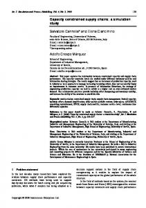
minimum matching cost. However, this approach ignores the service provider capacities. In our example, it assigns 5, 3, and 4 objects to q1 , q2 and q3 , respectively, violating the capacity constraints of q1 and q3 . The optimal CCA matching, on the other hand, would assign {p2 , p3 , p4 } to q1 , {p5 , ..., p9 } to q2 , and {p10 , p11 , p12 }Pto q3 , as shown by the three ellipses. In the general case q∈Q q.k 6= |P |, i.e., the customers may be fewer or more than the cumulative capacity of the service providers. CCA assigns every pj ∈ P to a qi ∈ Q, unless all service providers have reached their capacity. In Figure 1, for instance, p1 is not assigned to any qi , since they are all full. Conversely, it is possible that some service providers are not fully utilized. In any case, CCA computes the maximum size matching with the minimum assignment cost, subject to the capacity constraints.

Given a point set P of customers (e.g., WiFi receivers) and a point set Q of service providers (e.g., wireless access points), where each q ∈ Q has a capacity q.k, the capacity constrained assignment (CCA) is a matching M ⊆ Q × P such that (i) each point q ∈ Q (p ∈ P ) appears at most k times (at most once) in M , (ii) P the size of M is maximized (i.e., it comprises min{|P |, q∈Q q.k} pairs), and (iii) the total assignment cost (i.e., the sum of Euclidean distances within all pairs) is minimized. Thus, the CCA problem is to identify the assignment with the optimal overall quality; intuitively, the quality of q’s service to p in a given (q, p) pair is anti-proportional to their distance. Although max-flow algorithms are applicable to this problem, they require the complete distance-based bipartite graph between Q and P . For large spatial datasets, this graph is expensive to compute and it may be too large to fit in main memory. Motivated by this fact, we propose efficient algorithms for optimal assignment that employ novel edge-pruning strategies, based on the spatial properties of the problem. Additionally, we develop approximate (i.e., suboptimal) CCA solutions that provide a trade-off between result accuracy and computation cost, abiding by theoretical quality guarantees. A thorough experimental evaluation demonstrates the efficiency and practicality of the proposed techniques.

1.

p7

(k=5) p5

p9

p8

q1 (k=3) p4

p10

p3 p2 p1

INTRODUCTION

p11

q3 (k=3)

p12

Figure 1: Spatial assignment example

Consider a point set P of customers (e.g., WiFi receivers) and a point set Q of service providers (e.g., wireless access points). Suppose that each service provider q ∈ Q is able to serve at most q.k customers and every customer has at most one service provider. A subset M ⊆ Q × P is said to be a valid matching if (i) each point q ∈ Q (p ∈ P ) appears at most q.k times (at most once) in PM and (ii) the size of M is maximized (i.e., it is min{|P |, q∈Q q.k}). To quantify the quality of the matching M , we define its assignment cost as: X Ψ(M ) = dist(q, p) (1)

Besides the aforementioned wireless communication scenario, CCA arises in many resource allocation applications that require matching between users and facilities based on capacity constraints and spatial proximity. For instance, the municipality could assign children to schools (with certain capacity each) such that the average (or, equivalently, the summed) traveling distance of children to their schools is minimized. Another application (in welfare states) is the assignment of residents to designated, public clinics of given individual capacities. CCA can be reduced to the well-known minimum cost flow (MCF) problem in a complete distance-based bipartite graph between Q and P [1]. In the operations research literature [13], there is an abundance of MCF algorithms based on this reduction. These solutions, however, are only applicable to small-sized datasets and main memory processing. In particular, the best of them have a cubic time complexity (elaborated on in Section 2.2), and require that the bipartite graph (which contains |Q|·|P | edges) resides in memory. For moderate and large size datasets, this graph requires a pro-

(q,p)∈M

where dist(q, p) denotes the Euclidean distance between q and p. Intuitively, a high-quality matching should have low assignment cost. Figure 1 illustrates a scenario where P ={p1 , ..., p12 }, Q={q1 , q2 , q3 }, q1 .k = q3 .k = 3, and q2 .k = 5. Intuitively, assigning to each qi the points pj that fall inside its Voronoi cell (indicated by dashed lines in the figure) leads to the ∗

q2

p6

Supported by grant HKU 7155/06E from Hong Kong RGC. 1

hibitive amount of space (exceeding several times the typical memory sizes), and leads to an excessive computation cost as the CCA complexity increases with the number of graph edges. Motivated by the lack of CCA algorithms for large datasets, we develop efficient and highly scalable CCA techniques that produce an optimal assignment. Specifically, we assume that P resides in secondary storage, indexed by a spatial access method, while Q fits in main memory; in most real-world applications |Q| 8> HH22 vi .α + w(vi , vj ) then vj .α:=vi .α + w(u, v); vj .prev:=vi if vj ∈ Hd then update vj .α in Hd else if vj ∈ Hf then update vj .α in Hf else insert hvj , vj .αi into Hf

Example: We illustrate the PUA technique with an example. Figure 5(a) shows the current Esub edges between (some nodes of) sets Q and P , the α values of these nodes, and 7

Algorithm 6 Incremental ANN Search 1: 2: 3: 4: 5: 6: 7: 8: 9:

according to parameter δ. The dashed lines correspond to group MBR diagonals and their lengths cannot be longer than δ. The representatives of these groups are shown as gray points g1 , g2 and g3 . Assuming that all q ∈ Q have capacity q.k = 2, then the representative capacities are g1 .k = 6, g2 .k = 6, g3 .k = 8.

algorithm ANN(Group Gm , R-tree RP , Service provider qi ) while top entry in resi has key > key of top entry in Gm do de-heap top entry e from Hm if e is an directory entry of R-tree RP then visit node pointed by e and insert its entries into Hm else . E is a leaf level entry, i.e., a point p ∈ P for all qk in Gm do insert hp, dist(p, qk )i into resk de-heap top entry hpj , dist(pj , qi )i from resi return pj as the next NN of qi

4.

G2

G1 q1

APPROXIMATE METHODS

q2 q3 g–1

q6

q5

q8 g–3 q7

Time-critical applications may favor fast answers over exact ones. This motivates us to develop approximate CCA solutions. In this section, we propose a methodology that provides a tunable trade-off between result accuracy and response time, and comes with theoretical guarantees for the assignment cost. Our general approach consists of three phases. The first one is the partitioning phase, in which we form groups Gm of either the points in Q or points in P , so that the diagonal of their MBR does not exceed a threshold δ. Parameter δ is used to control the quality of the assignment; the smaller δ is the better the computed matching approximates the optimal. The second phase, called concise matching, solves optimally a small CCA problem extracting one representative point per group Gm and using the set of representatives as the set of service providers (customers). Finally, the refinement phase uses the assignment produced in the previous step to derive a matching on the entire sets P and Q. Sections 4.1 and 4.2 describe two methods, called Service Provider Approximation (SA) and Customer Approximation (CA). SA and CA follow different approaches for partitioning and subsequent concise matching. Specifically, SA groups the service providers and solves concise matching in the entire P , while CA groups the customers and performs concise matching in the entire Q.4 Section 4.3 describes refinement techniques that could be used with either SA or CA. Finally, Section 4.4 provides error bounds for both approaches.

4.1

g–2

q4

q10 G3

q9

Figure 6: Service provider partitioning The resulting representatives form set Q0 which is used as an approximation of Q. The concise matching of SA solves an exact CCA problem over Q0 and P . This step is performed by the IDA algorithm described in Section 3.3, because (as will be demonstrated by our experiments) it is the most efficient among the exact methods. The matching M 0 produced by this step will be refined into the final matching M using one of the techniques presented in Section 4.3.

4.2

Customer Approximation

CA is similar to SA, but groups customers instead of service providers. Recall that P is indexed by an R-tree. We first initialize a set S of customer groups to ∅. Given parameter δ, we traverse the R-tree. Starting from the root entries, we compare the MBR diagonal of each of them with δ. If the diagonal of entry e is smaller than or equal to δ, we insert it into S (the corresponding group of customers are those in the subtree rooted at e). Otherwise (i.e., e’s diagonal is larger than δ), we visit the corresponding node and recursively repeat this procedure for its entries. R-tree leaves are an exception to this procedure. In particular, if δ is small, it is possible that we reach an entry e corresponding to an R-tree leaf whose diagonal is larger than δ. An option would be to insert into S all points in e, but this would result in a large S. Thus, we handle e as follows. We conceptually split its MBR into two equal halves on its longest dimension. We repeat this process until the diagonal of each partition becomes smaller than or equal to δ. Then, we insert the resulting conceptual entries into S. Upon termination of the above procedure, all entries in S have diagonal smaller than δ and the union of points in their subtrees is the entire P . The size of S, however, can be reduced (without violating the δ constraint) by an extra step that merges its contents. Specifically, we use a procedure similar to SA and group entries in S into conceptual hyperentries whose diagonal does not exceed δ. Let S be the final set of entries (conceptual or not). We produce a set P 0 of customer representatives as follows. For each e ∈ S we derive a representative point g located at the geometric centroid of e. The representative has weight g.w equal to the number of points in the subtree of e. To exemplify CA partitioning, assume that the R-tree of P and parameter δ are as shown in Figure 7 (the R-tree is illustrated both in the spatial domain and as stored on the disk). We first access the root, and consider its entries e1 and e2 . Entry e2 has smaller diagonal than δ and is inserted

Service Provider Approximation

Partitioning in SA is performed on set Q. The points q ∈ Q are sorted according to their Hilbert values and processed in this order. We start with zero service provider groups. Each point q, in turn, is inserted into an existing group Gm so that the diagonal of Gm ’s MBR does not exceed δ. If no such group is found, then a new group is formed to include q. The process is repeated until all q ∈ Q are grouped. We proceed to concise matching by extracting one representative point per group. The representative point gm of P a group Gm has capacity gm .k = q∈Gm q.k and is located at its geometric centroid ; each coordinate of gm is equal to the weighted average of points inside Gm . Weighting is performed according to the capacities q.k of points P q ∈ Gm , e.g., the x-coordinate gm .x of gm is P 1 q.k q∈Gm (q.x · q.k). q∈Gm

Figure 6 shows a scenario where Q = {q1 , ..., q10 }. Assume that SPP produces the illustrated groups G1 , G2 , G3 4

We note here that we attempted to combine SA and CA (i.e., to group both Q and P ), but this led to a very poor matching. Thus, we omit this hybrid method. 8

4.4

into S. This is not the case for e1 , whose pointed entries are loaded from the disk. Among e1 ’s entries, e4 and e5 satisfy the diagonal condition and are included in S. On the other hand, e3 is a leaf and still has diagonal larger than δ. Thus, we conceptually divide it into two new entries on its long dimension (i.e., x dimension). The resulting e3,1 and e3,2 have small enough diagonal and are placed into S. Entries inserted into S are shown shaded. In the last step, we merge entries into larger ones (while still satisfying the δ condition); e4 and e5 form a hyper-entry whose boundaries are shown dashed. Every entry in the final S implicitly defines a group of customers Gm . Set P 0 contains the representatives of the final entries in S, i.e., P 0 = {g1 , g2 , g3 , g4 }. e2 e7 e6

g–4

g–1 e3,1

e1

Let M be the matching computed by SA and MCCA be the optimal matching. The assignment cost error of M is: Err(M ) = Ψ(M ) − Ψ(MCCA ),

Theorem 3. The assignment error of SA is upper bounded by 2 · γ · δ. Proof. Note that approximate matching M has the full size γ, since concise matching leaves customers unassigned only if all service providers are fully utilized (i.e., they have reached their capacity). From the optimal matching MCCA , 0 we derive another matching MCCA by replacing each pair (q, p) ∈ MCCA with pair (g, p), where g is the representative of q’s group. After the replacement, the cost of each pair increases/decreases by at most δ (since δ is the maximum possible distance between q and the weighted centroid g). 0 ) ≤ Ψ(MCCA ) + γ · δ. Thus, Ψ(MCCA 0 is not necessarily the optimal matching Note that MCCA between Q0 (i.e., the set of service provider representatives) and P . Let M 0 be the optimal matching between Q0 and 0 ). Combining the two P . We know that Ψ(M 0 ) ≤ Ψ(MCCA inequalities, we derive Ψ(M 0 ) ≤ Ψ(MCCA ) + γ · δ. SA replaces the pairs of M 0 heuristically to form the final matching M , incuring a maximum error of δ per pair. Hence, Ψ(M ) ≤ Ψ(M 0 ) + γ · δ. From the last two inequalities, we infer that Ψ(M ) ≤ Ψ(MCCA ) + 2 · γ · δ.

R-tree root e1 e2

g–2 e3,2 e4

g–3

e5

e1 e3 e4 e5

e2 e6 e7

Figure 7: Customer partitioning In the concise matching phase, CA computes the optimal matching M 0 between P 0 and Q. This is performed in main memory (where P 0 and Q reside) using IDA. Note that in this setting points in P 0 also have capacities (the representative weights). This is not a problem, since IDA (as well as RIA and NIA) can handle capacities in the customer side of the flow graph too. The difference is that M 0 may assign “instances” of a representative to multiple service providers.

4.3

(4)

where Ψ(M ) and Ψ(MCCA ) are defined as in Equation 1. We showPthat Err(M ) is at most 2 · γ · δ, where γ = min{|P |, q∈Q q.k}. Thus, we are able to control the assignment cost error through parameter δ.

δ

e3

Assignment Cost Guarantee

The assignment error of CA is bounded as follows.

Refinement Phase

Theorem 4. The assignment error of CA is upper bounded by γ · δ.

In both SA and CA, we are given a matching M 0 between one approximate set (i.e., Q0 or P 0 ) and one original set (P or Q, respectively). In either case, M 0 specifies for each group Gm of service providers (customers) which customers (instances of service providers) are assigned to it. In other words, in both SA and CA the refinement phase has to solve several smaller problems of assigning a set of customers P 00 to a set of service providers Q00 (where the number of points p ∈ P 00 to be assigned to each q ∈ Q00 is given by the concise matching phase). We could run an exact algorithm for each of these smaller problems. This, however, is expensive. Instead, we propose the following two heuristics5 , receiving smalls sets P 00 and Q00 as input.

Proof. The proof follows the same lines as that of SA, the difference being that the maximum possible distance between a customer p and its group representative g is 2δ (since g is always the geometric centroid of p’s group MBR).

5.

EXPERIMENTS

This section empirically evaluates the performance of our algorithms. All methods were implemented in C++ and experiments were performed on a Pentium D 3.0GHz machine, running on Ubuntu 7.10. Section 5.1 describes the datasets, the parameters under investigation, and other settings used in our evaluation. In Section 5.2 we study the performance of our algorithms on optimal CCA computation. Section 5.3 explores the efficiency and assignment cost error of our techniques on approximate CCA computation.

NN-based refinement: This approach computes the (next) NN of each q ∈ Q00 in a round-robin fashion in set P 00 . When discovering the NN p of service provider q, we include pair (q, p) in the final assignment M and remove p from P 00 . If q has reached its number of instances to be assigned to P 00 , we also delete q from Q00 .

5.1

Data Generation and Problem Settings

The CCA problem takes two spatial datasets as input: the service provider set Q and the customer set P . Both datasets were generated on the road map of San Francisco (SF) [3], using the generator of [15]. In particular, the points fall on edges of the road network, so that 80% of them are spread among 10 dense clusters, while the remaining 20% are uniformly distributed in the network. This dataset selection simulates a real situation where some parts of the city are denser than others. To establish the generality of our

Exclusive NN refinement: According to this strategy, we identify the p ∈ P 00 with the minimum distance from any q ∈ Q00 that has not reached its number of instances to be assigned to P 00 (according to M 0 ). We insert into the final assignment M the corresponding pair (q, p) and proceed with the next customer in P 00 . 5 We experimented with several other alternatives but these two methods were both efficient and quite accurate.

9

1.0e9

200

250

0 300

RIA NIA IDA

150

RIA NIA IDA

100

RIA NIA IDA

50

RIA NIA IDA

size of subgraph

time (s)

1,000

k=20

k=40

k=80

k=160

k=320

(b) total time

Figure 9: Performance vs. k, |Q| = 1K, |P | = 100K

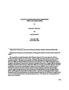
Figure 9(b) shows the total execution time in the previous experiment, and breaks it into I/O and CPU cost. The I/O time depends primarily on (and thus follows the increasing trend of) |Esub |. The CPU time also rises with k, since the flow graph size and the number of iterations γ increase with k. For large k values, however, the increase for RIA is not as steep, while for INA and NIA the CPU cost drops slightly. This happens because the capacity constraint is looser and, essentially, the problem becomes easier. NIA has lower CPU time than RIA because NIA adds new edges one-by-one and keeps the subgraph small. Note that even for large k (where the final |Esub | is similar for RIA and NIA), the early iterations of NIA run on a smaller Esub which increases only towards its final iterations. On the other hand, IDA is faster than NIA because (i) Theorem 2 computes the first assignments fast and (ii) the utilization of full service providers (i.e., with non-zero qi .α values) avoids unnecessary edge insertions into Esub and leads to earlier termination. The next experiment investigates the effect of service provider cardinality |Q| (in Figure 10). In general, the relative performance of the algorithms is consistent with our observations in Figure 9; IDA prunes more edges than NIA/RIA when k · |Q| < |P |. The cost of the problem increases with |Q|, but saturates when k · |Q| > |P |, since the optimal assignment is found before long edges (from service providers to their furthest neighbors) are examined. 8,000

1.0e8

7,000

1.0e7

6,000

1.0e6

5,000

1.0e5 1.0e4 RIA NIA IDA FULL

320

1.0e1

k

2,000 1,000 0

1.0e0 0

Figure 8: CPU time vs. k, |Q| = 250, |P | = 25K

1

2

3 |Q| (kilo)

(a) |Esub | In the remaining experiments, we focus on disk-based P and large problem instances, excluding the inapplicable SSPA. Figure 9(a) shows the subgraph size Esub as a function of k (setting |Q| and |P | to their default values). We include the complete bipartite graph size |EF U LL | = |Q|·|P | as a reference (indicated by FULL). Due to the application of Theorem 1, our algorithms (RIA, NIA, IDA) use/store only a fragment of the complete bipartite graph. IDA explores fewer edges than RIA and NIA for small values of k. The reason behind this is that for k · |Q| < |P |, providers are likely to become full early and the tighter bounds of IDA over NIA/RIA can be effectively utilized. On the other hand, if k·|Q| > |P |, few or no providers become full, so IDA does not achieve additional pruning compared to NIA/RIA.

4

3,000

5

RIA NIA IDA

1.0e2

4,000

RIA NIA IDA

1.0e3

CPU time I/O time

RIA NIA IDA

10

1.0e9

RIA NIA IDA

size of subgraph

CPU time (s)

3,000

k

100

160

RIA NIA IDA FULL

(a) |Esub |

SSPA RIA NIA IDA

80

CPU time I/O time

2,000

1.0e3

0

SSPA requires that the complete flow graph is stored in main memory (as described in Section 2.2). For our default setting this leads to space requirements that exceed several times the available system memory. To provide, however, an intuition about (i) the inherent complexity of the problem and (ii) the relative performance of SSPA versus our algorithms, we experiment on a smaller problem; we generate P and S as described in Section 5.1, with |Q| = 250 and |P | = 25K, so that the flow graph fits in main memory. For RIA, NIA, and IDA, P is indexed by a memory-based R-tree. SSPA does not utilize an index, as it involves no spatial searches. Figure 8 shows the CPU time (in logarithmic scale) versus capacity k in this small problem. Our methods are one to three orders of magnitude faster than SSPA. We postpone the explanation of the observed trends for Figure 9 (with disk-resident P ), but stress the excessive time requirements of SSPA and the efficiency of our methods.

40

4,000

1.0e0

5.2 Experiments on Optimal Assignment

20

1.0e4

1.0e1

Table 2: System parameters

1

1.0e5

1.0e2

Range 0.25, 0.5, 1, 2.5, 5 25, 50, 100, 150, 200 20, 40, 80, 160, 320 10, 20, 40, 80, 160

1,000

1.0e6

RIA NIA IDA

Default 1 100 80 SA: 40, CA: 10

5,000

1.0e7

time (s)

Parameter |Q| (in thousands) |P | (in thousands) Capacity k Diagonal δ

6,000

1.0e8

RIA NIA IDA

methods, we also present results for different distributions. All datasets are normalized to lie in a [0, 1000]2 space. By default, the capacity k of all q ∈ Q is 80 and the dataset cardinalities are |Q|=1K and |P |=100K. Parameter θ of RIA is fine-tuned (and set to 0.8), for fairness in the comparison with NIA and IDA. Table 2 shows the parameters under investigation. We assume that the service provider dataset Q is small enough to fit in main memory. Each P dataset is indexed by an R-tree with 1Kbyte page size. We use an LRU buffer with size 1% of the tree size. We record the memory usage (i.e., |Esub |, number of edges in the subgraph) and the CPU time. Also, we measure I/O time by charging 10ms per page fault [10].

|Q|=0.25 |Q|=0.5

|Q|=1

|Q|=2.5

|Q|=5

(b) total time

Figure 10: Performance vs. |Q|, k = 80, |P | = 100K Figure 11 investigates the effect of |P |. When |P | increases, the complete flow graph grows but the subgraph explored by our algorithms shrinks. Intuitively, if there are too many customers, the NNs of each service provider are closer, and stand a higher chance to be assigned to it; i.e., the problem becomes easier and fewer Esub edges (and, thus, computations) are needed. However, for |P | = 200K the customer R-tree has one more level than smaller cardinalities, incurring more I/Os and a higher overall cost. Note that the difference of IDA from RIA/NIA grows as |P | becomes larger compared to k·|Q| (for the reasons mentioned earlier). 10

1.0e3

RIA NIA IDA FULL

1.0e2 1.0e1 1.0e0 0

50

100 |P| (kilo)

150

200

(a) |Esub |

|P|=25

|P|=50 |P|=100 |P|=150 |P|=200

Experiments on Approximate Assignment

In this section, we evaluate the accuracy of our approximate CCA methods (i.e., SA and CA) presented in Section 4, and compare their execution time with IDA (the best exact algorithm). We measure the accuracy of an approximate matching M by Ψ(M )/Ψ(MCCA ), where MCCA is the optimal assignment. For each of SA and CA, we implemented both the NN-based and exclusive NN refinement techniques (indicated by “N” and “E” after SA or CA in chart labels). Figure 14 shows the approximation quality and the running time as a function of the diagonal parameter δ (used in the partitioning phase). Observe that the CA variants are significantly better than those of SA in terms of quality and efficiency for all values of δ. An exception is δ = 10 where SA achieves a better approximation, at a cost, however, that is comparable to IDA (since almost every provider forms a group by itself). As expected, accuracy and execution cost drop with δ. CA with as small δ as 10 achieves great performance improvement over IDA, while producing a matching only marginally worse than the optimal.

RIA NIA IDA

1.0e4

RIA NIA IDA

1.0e5

5.3 CPU time I/O time

RIA NIA IDA

1.0e6

time (s)

size of subgraph

1.0e7

1,800 1,600 1,400 1,200 1,000 800 600 400 200 0

RIA NIA IDA

1.0e8

RIA NIA IDA

1.0e9

(b) total time

Figure 11: Performance vs. |P |, k = 80, |Q| = 1K

So far we assumed that all service providers have equal capacities q.k. Figure 12 compares the algorithms for problems where the providers have different k, taken randomly from the ranges shown as labels on the horizontal axis. The results are similar to those in Figure 9; i.e., mixed k values do not affect the effectiveness of our pruning techniques. 1.0e9 1.0e8 7,000

2,000

100

0

20,000

80 100 120 140 160 Diagonal

Quality

CPU time I/O time

2,500

3 2.5

1,000 500

(a) |Esub |

RIA NIA IDA

0

100

150 k

200

(a) quality RIA NIA IDA

CvsC

0

50

UvsU

UvsC

CvsU

CvsC

250

300

CPU time I/O time

1,500

1.5 0

RIA NIA IDA

CvsU

d=160

2,000

2

1

RIA NIA IDA

UvsC

data distributions

d=80

3,000

SAN SAE CAN CAE

3.5

5,000 UvsU

d=40

3,500

4

10,000

1.0e2 1.0e1

d=20

(b) total time

15,000

1.0e4 1.0e3

d=10

In the remaining experiments, we set δ to 40 for SA, and to 10 for CA, as those values achieve the best efficiency/accuracy trade-off. We evaluate the approximate solutions using the defaults and ranges in Table 2 for k, |Q|, and |P |. In Figure 15, we vary k and observe that the approximation quality improves with it. As k increases, the providers are assigned more distant customers; i.e., both Ψ(M ) and Ψ(MCCA ) grow. On the other hand, the provider/customer group MBRs remain constant (as δ is fixed) and, hence, the relative error of a suboptimally assigned customer drops. The CA variants are more robust (i.e., less affected by k) than SA, with a 12% error in the default, and 23% in the worst case. The execution time of SA/CA follows the trend of IDA, due to their IDA-based concise matching (but both SA and CA are several times faster).

25,000

1.0e6 1.0e5

60

Figure 14: Quality vs. δ (default k, |Q|, |P |)

times (s)

size of subgraph

RIA NIA IDA

40

(a) quality

Figure 13 compares the algorithms when Q and P follow varying distributions; uniform (U) places points uniformly in the SF network, while clustered (C) generates datasets in the way described in Section 5.1. For example, label “UvsC” on the horizontal axis corresponds to uniform service providers and clustered customers. We observe that the cost for computing the optimal assignment increases considerably when the two sets are distributed differently. If Q is uniform and P is clustered (e.g., customers gather in central squares during New Year’s Eve), some providers are far from their nearest customer clusters and compete for points far from them, thus increasing the size of the examined subgraph. If Q is clustered and P is uniform (e.g., service providers concentrate around certain regions), the providers cannot fill their capacities with customers near them, and need to expand their search ranges very far. In both cases, NIA is slower than RIA, because the incremental edge retrieval (that is slower than a batch range-based insertion in RIA) is invoked numerous times.

1.0e0

20

(b) total time

Figure 12: Perf. for mixed k, |Q| = 1K, |P | = 100K

1.0e8 1.0e7

0

1

IDA SAN SAE CAN CAE

20~60 40~120 80~240 160~480

IDA SAN SAE CAN CAE

(a) |Esub |

10~30

IDA SAN SAE CAN CAE

k

200

IDA SAN SAE CAN CAE

300

IDA SAN SAE CAN CAE

250

IDA SAN SAE CAN CAE

200

400

IDA SAN SAE CAN CAE

150

500

IDA SAN SAE CAN CAE

100

2

time (s)

50

2.5

300

RIA NIA IDA

0

600

1.5

RIA NIA IDA

0

1.0e0

CPU time I/O time

700

1,000 RIA NIA IDA

1.0e1

3,000

RIA NIA IDA

1.0e2

4,000

800

IDA SAN SAE CAN CAE

RIA NIA IDA FULL

RIA NIA IDA

1.0e3

Quality

1.0e4

900

SAN SAE CAN CAE

3

IDA SAN SAE CAN CAE

5,000

1.0e5

3.5

CPU time I/O time

time (s)

6,000

1.0e6 time (s)

size of subgraph

1.0e7

k=20

k=40

k=80

k=160

k=320

(b) total time

Figure 15: Performance vs. k, |Q| = 1K, |P | = 100K

(b) total time Figure 16 evaluates the approximation methods for various service provider cardinalities. Again, CA is more accurate than SA, while there are only marginal differences

Figure 13: Different distributions (default k, |Q|, |P |)

11

6.

between its CAN and CAE variants. The quality of CA worsens with |Q|, because the more service providers around a customer group, the higher the chances for a suboptimal pair in M . On the other hand, in SA the provider groups have a fixed maximum diagonal δ, but their density varies. Very low or very large densities lead to poor approximations.

In this paper, we identify the capacity constrained assignment (CCA) problem, which retrieves the matching (between two spatial point sets) with the lowest assignment cost, subject to capacity constraints. CCA is important to applications involving assignment of users to facilities based on spatial proximity and capacity limitations. We present efficient CCA techniques that expand the search space incrementally and effectively prune it. We also develop approximate CCA solutions that provide a trade-off between computation cost and matching quality. According to our experimental results, IDA is the best algorithm for the exact CCA problem, while CA is the method of choice for approximate CCA matching. In our assumed setting, the set of service providers fits in main memory, while the customers are indexed by a diskbased R-tree. In the future, we plan to extend our framework to the scenario where both sets are disk-resident, incorporating hash-based techniques.

4,000

2.2

CPU time I/O time

3,000 2,500 time (s)

2 1.8 1.6

2,000 1,500

1.4

1,000

2

3 |Q| (kilo)

4

5

(a) quality

IDA SAN SAE CAN CAE

1

IDA SAN SAE CAN CAE

0

IDA SAN SAE CAN CAE

0

1

IDA SAN SAE CAN CAE

500

1.2

IDA SAN SAE CAN CAE

Quality

3,500

SAN SAE CAN CAE

|Q|=0.25

|Q|=0.5

|Q|=1

|Q|=2.5

|Q|=5

(b) total time

Figure 16: Performance vs. |Q|, k = 80, |P | = 100K In Figure 17, we investigate the effect of |P |. The increase of |P | reduces the accuracy of SA; as the space around every provider group becomes denser with customers, the potential for suboptimal matchings becomes higher. The accuracy of CA is affected to a lesser degree by |P |. The slight error increase is because CA groups more customers together, implying a coarser partitioning and worse approximation.

7.

8.

1,200

SAN SAE CAN CAE

800

2 1.8 1.6

600 400

1.4

200

200

(a) quality

IDA SAN SAE CAN CAE

150

IDA SAN SAE CAN CAE

100 |P| (kilo)

IDA SAN SAE CAN CAE

50

IDA SAN SAE CAN CAE

0

0

IDA SAN SAE CAN CAE

1.2 1

|P|=25

|P|=50

|P|=100

|P|=150

|P|=200

(b) total time

Figure 17: Performance vs. |P |, k = 80, |Q| = 1K Figure 18 compares the approximate methods for different Q and P distributions. CA performs best in terms of running time for all distributions. CA is also more accurate than SA for similarly distributed Q and P (which is the case in most applications). For differently distributed Q and S, the quality of SA and CA is comparable, and close to optimal. To summarize the approximation experiments, CA typically computes a near-optimal matching, while being orders of magnitude faster than IDA. 7,000

SAN SAE CAN CAE

1.6 1.5

time (s)

1.3 1.2

4,000 3,000 2,000

1.1 CvsU

data distributions

(a) quality

CvsC

0

IDA SAN SAE CAN CAE

UvsC

IDA SAN SAE CAN CAE

1,000

UvsU

IDA SAN SAE CAN CAE

1

CPU time I/O time

IDA SAN SAE CAN CAE

Quality

1.4

6,000 5,000

UvsU

UvsC

CvsU

CvsC

REFERENCES

[1] R. K. Ahuja, T. L. Magnanti, and J. B. Orlin. Network Flows: Theory, Algorithms, and Applications. Prentice Hall, first edition, 1993. [2] N. Beckmann, H.-P. Kriegel, R. Schneider, and B. Seeger. The R*-tree: An Efficient and Robust Access Method for Points and Rectangles. In SIGMOD, 1990. [3] T. Brinkhoff. A Framework for Generating Network-Based Moving Objects. GeoInformatica, 6(2):153–180, 2002. [4] A. Corral, Y. Manolopoulos, Y. Theodoridis, and M. Vassilakopoulos. Closest Pair Queries in Spatial Databases. In SIGMOD, 2000. [5] A. V. Goldberg and R. Kennedy. An Efficient Cost Scaling Algorithm for the Assignment Problem. Mathematical Programming, 71:153–177, 1995. [6] A. Guttman. R-Trees: A Dynamic Index Structure for Spatial Searching. In SIGMOD, 1984. [7] G. R. Hjaltason and H. Samet. Distance Browsing in Spatial Databases. ACM Trans. Database Syst., 24(2):265–318, 1999. [8] J. Munkres. Algorithms for the Assignment and Transportation Problems. Journal of the Society of Industrial and Applied Mathematics, 5(1):32–38, 1957. [9] T. K. Sellis, N. Roussopoulos, and C. Faloutsos. The R+-Tree: A Dynamic Index for Multi-Dimensional Objects. In VLDB, 1987. [10] A. Silberschatz, H. F. Korth, and S. Sudarshan. Database System Concepts. McGraw-Hill, fifth edition, 2005. ¨ coluk. Incremental Assignment [11] I. H. Toroslu and G. U¸ Problem. Inf. Sci., 177:1523–1529, 2007. [12] L. H. U, N. Mamoulis, and M. L. Yiu. Continuous Monitoring of Exclusive Closest Pairs. In SSTD, 2007. [13] J. Vygen. Approximation Algorithms for Facility Location Problems (Lecture Notes). University of Bonn, 2004. [14] R. C.-W. Wong, Y. Tao, A. Fu, and X. Xiao. On Efficient Spatial Matching. In VLDB, 2007. [15] M. L. Yiu and N. Mamoulis. Clustering objects on a spatial network. In SIGMOD, 2004.

CPU time I/O time

1,000

time (s)

Quality

2.2

REPEATABILITY ASSESSMENT RESULT

All the results in this paper were verified by the SIGMOD repeatability committee. Code and/or data used in the paper are available at: http://www.sigmod.org/codearchive/sigmod2008/

2.6 2.4

CONCLUSION

(b) total time

Figure 18: Different distributions (default k, |Q|, |P |)

12