Dec 11, 2013 - where f(l0,...,li,mi) is a joint probability: f(l0,...,li,mi) = P(li,mi|l0,...,liâ1) ... of Ps(Ï) that it is maximized if li needs to be as less as possible, i.e., ...
Dynamic Control of Coding for Progressive Packet Arrivals in DTNs Eitan Altman, Lucile Sassatelli, Francesco De Pellegrini
To cite this version: Eitan Altman, Lucile Sassatelli, Francesco De Pellegrini. Dynamic Control of Coding for Progressive Packet Arrivals in DTNs. IEEE Transactions on Wireless Communications, Institute of Electrical and Electronics Engineers (IEEE), 2013, 12 (2), pp.725-735. .
HAL Id: hal-00917413 https://hal.inria.fr/hal-00917413 Submitted on 11 Dec 2013
HAL is a multi-disciplinary open access archive for the deposit and dissemination of scientific research documents, whether they are published or not. The documents may come from teaching and research institutions in France or abroad, or from public or private research centers.
L’archive ouverte pluridisciplinaire HAL, est destin´ee au d´epˆot et `a la diffusion de documents scientifiques de niveau recherche, publi´es ou non, ´emanant des ´etablissements d’enseignement et de recherche fran¸cais ou ´etrangers, des laboratoires publics ou priv´es.
1
Dynamic control of Coding for general packet arrivals in DTNs Eitan Altman, Francesco De Pellegrini and Lucile Sassatelli
Abstract Delay tolerant Networks (DTNs) leverage the mobility of relay nodes to compensate for lack of persistent connectivity. In order to decrease message delivery delay, the information to be transmitted can be replicated in the network. For general packet arrivals at the source and two-hop routing, we derive performance analysis of replication-based routing policies and study their optimization. In particular, we find out the conditions for optimality in terms of probability of successful delivery and mean delay and devise optimal policies, so-called piecewise threshold policies. We account for linear block-codes as well as rateless random linear coding to efficiently generate redundancy, as well as for an energy constraint in the optimization. We numerically assess the higher efficiency of piecewise threshold policies compared with other policies by developing heuristic optimization of the thresholds for all flavors of coding considered. Index Terms Delay Tolerant Networks, Mobile Ad Hoc Networks, Optimal Scheduling, Rateless codes, Network coding
I. I NTRODUCTION Delay Tolerant Networks (DTNs) leverage contacts between mobile nodes and sustain end-to-end communication even between nodes that do not have end-to-end connectivity at any given instant. In this context, contacts between DTN nodes may be rare, for instance due to low densities of active nodes, so that the design of routing strategies is a core step to permit timely delivery of information to a certain destination with high probability. When mobility is random, i.e., cannot be known beforehand, this is obtained at the cost of many replicas of the original information, a process which consumes energy and memory resources. Since many relay nodes (and thus network resources) may be involved in ensuring successful delivery, it becomes crucial to design efficient resource allocation and data storage protocols. The basic questions are then: (i) transmission policy: when the source is in contact with a relay node, should it transmit a packet to the relay?
2
(ii) scheduling: if yes, which packet should a source transfer? In the basic scenario, the source has initially all packets. Under this assumption it was shown in [1] that the transmission policy has a threshold structure: it is optimal to use all opportunities to spread packets till some time σ and then stop. This policy resembles the well-known “Spray-and-Wait” policy [2]. In this work we assume a more general arrival process of packets: they need not to be simultaneously available for transmission initially, i.e., when forwarding starts, as assumed in [1]. This is the case when large multimedia files are recorded at the source node that sends them out without waiting for the whole file reception to be completed. Contributions. This paper focuses on general packet arrivals at the source and two-hop routing. The contributions are fourfold: •
For work-conserving policies, we find out the conditions for optimality in terms of probability of successful delivery and mean delay.
•
We prove that work-conserving policies are always outperformed by so-called piecewise threshold policies. These policies are the extension of threshold policies derived in [1], [3], for the case of general packet arrival at the source.
•
We extend the above analysis to the case where redundant packets are coded packets, generated both with linear block-codes and rateless coding. We also account for an energy constraint in the optimization.
•
We illustrate numerically the higher efficiency of piecewise threshold policies compared with workconserving policies by developping heuristic optimization of the thresholds for all flavors of coding considered.
More in details, assume t = (t1 , . . . , tK ) are the arrival times of the K packets at the source, t1 ≤ t2 ≤ . . . ≤ tK . Owing to progressive arrivals, work-conserving policies (i.e., when the source sends a packet with probability 1 all the time) can be suboptimal, in contrast to [1], [3]. Defining couples (si , pi ) for i = 1, . . . , K, where si are thresholds in [ti , ti+1 ] and pi are probabilities such that the source sends with probability pi only between ti and si , we are able to prove analytically that piecewise threshold policies, defined by s′i with pi = 1, for all i = 1, . . . , K, always outperform other kind of policies. Related Work. Papers [4] and [5] propose a technique to erasure code a file and distribute the generated code-blocks over a large number of relays in DTNs. The use of erasure codes is meant to increase the efficiency of DTNs under uncertain mobility patterns. In [5] the performance gain of the coding
3
scheme is compared to simple replication, i.e., when additional copies of the same file are released. The benefit of erasure coding is proved by means of extensive simulations and for different routing protocols, including two hop routing. In [4], the authors address the case of non-uniform encounter patterns, and they demonstrate strong dependence of the optimal successful delivery probability on the way replicas are distributed over different paths. The authors evaluate several allocation techniques; also, the problem is proved to be NP–hard. The paper [6] proposes general network coding techniques for DTNs. In [7] ODE based models are employed under epidemic routing; in that work, semi-analytical numerical results are reported describing the effect of finite buffers and contact times; the authors also propose a prioritization algorithm. The same authors in [8] investigate the use of network coding using the Spray-and-Wait algorithm and analyze the performance in terms of the bandwidth of contacts, the energy constraint and the buffer size. The paper [9] addresses the design of stateless routing protocols based on network coding, under intermittent end-to-end connectivity. A forwarding algorithm based on network coding is specified, and the advantage over plain probabilistic routing is proved when delivering multiple packets. The structure of the paper is the following. In Sec. II we introduce the network model and the optimization problems tackled in the rest of the paper. Sec. III and Sec. IV describe optimal solutions in the case of work-conserving and not work-conserving forwarding policies, respectively. Sec. V addresses the case of energy constraints. Sec. VI performance analysis of linear block-coding. Rateless coding techniques are presented in Sec. VII. Sec. VIII provides a numerical analysis, and Sec. IX concludes the paper. II. T HE
MODEL
[TABLE 1 about here.] The main symbols used in the paper are reported in Tab. I. Consider a network that contains N + 1 mobile nodes. We assume that two nodes are able to communicate when they come within reciprocal radio range and communications are bidirectional, and that the duration of such contacts is sufficient to one packet in each direction. Also, let the time between contacts of pairs of nodes be exponentially distributed. The validity of this model been discussed in [10], and its accuracy has been shown for a number of mobility models (Random Walker, Random Direction, Random Waypoint). Following the notation of [11], let β be the intra-meeting intensity, i.e., the mean number of meetings between any two given nodes per unit
4
of time. Let λ be the inter-meeting intensity (mean number of meetings between one given node and any other nodes within unit time). We have λ = βN because we consider the density of nodes is constant, so is λ, when N increases. That matches to the fact that the number of nodes that fall within radio range per unit of time remains constant if the density of nodes does. A file is transmitted from a source node to a destination node, and decomposed into K packets. The source of the file receives the packets at some times t1 ≤ t2 ≤ ... ≤ tK . ti are called the arrival times. We assume that the transmitted file is relevant during some time τ , i.e., all the packets should arrive at the destination by time t1 + τ . Furthermore, we do not assume any feedback that allows the source or other mobiles to know whether the file has made it successfully to the destination within time τ . We consider two-hop routing: a packet can go only through one relay. The forwarding policy of the source is as follows. If at time t the source encounters a mobile which does not have any packet, it gives P it packet i with probability ui (t). Clearly, u ≤ 1 where u = i ui (t). Also, there is an obvious constraint
that ui (t) = 0 for t ≤ ti .
b (N ) (t) be a K dimensional vector whose components are X b (N ) (t), for i = 1, . . . , K. Here, X b (N ) (t) Let X i i
stands for the fraction of mobile nodes (excluding the destination) that have at time t a copy of packet b (N ) (t). This models the spreading process of the i-th b (N ) (t) = PK X i, in a network of size N. Let X i i=1
packet in the network: in the following we will refer to fluid approximations that describe the dynamics of the fraction of infected nodes. The validity of such approximation is detailed below. In particular, owing to the dependence of this process on β, and hence on N, we cannot readily apply the convergence
results of [12]. Below we detail the approach based on [13] so as to derive analytical expressions of some performance measures.
A. Performance measures: mean-field approximations Consider time t sampled over the discrete domain, i.e., t ∈ N. For our case, the drift defined in [13] is � � b (N ) (t + 1) − X b (N ) (t)|X b (N ) (t) = m . f (N,i) (m) = E X i i Owing to the model, we have f (N,i) (m) = ui (t)β(1 − m). By checking condition H2 of [13], there exists a function ǫ(N) such that limN →∞ ǫ(N) = 0 and, for all m ∈ [0, 1], limN →∞
f (N,i) (m) ǫ(N )
= fi (m) . Indeed,
ǫ(N) = β(N)/λ, fulfills the condition, since limN →∞ β = 0 and λ is a constant in N. This interaction process is then said to have vanishing intensity [13]. In such cases, Bena¨ım and Le Boudec have shown
5
˜ (N ) (r) converges for large N, in [13] that, provided that we change the time scale, the re-scaled process X i in mean-square, to a deterministic dynamic system which is the solution of a certain Ordinary Differential ˜ (N ) (r) is defined as a continuous time process by Equation (ODE). More precisely, X i X ˜ (N ) (tǫ(N)) = X b (N ) (t) for all t ∈ N i i X ˜ (N ) (r) is affine on r ∈ [tǫ(N); (t + 1)ǫ(N)] i ˜ (N ) (r) converges to a deterministic process X ¯ (N ) (r) which is the solution of Then X i i
(N)
¯ dX (r) i dr
¯ (N ) ) . = fi (X
Let us denote ǫ(N) by ǫ in what follows for lighter notation. Let us define u¯i (r) as the re-scaled version ˜ (N ) (r). The fraction of nodes holding packet i is approximated, for of ui (t), in the same way as for X i (N)
large N, by the solution of:
¯ dX (r) i dr
=
u ˜i (r)β (1 ǫ
¯ (N ) (r)), −X
¯ (N ) (r) = 1 − (1 − z) exp X i In general, the term
β ǫ
�
β − ǫ
¯ (N ) (0) = z . We get X i Z
r 0
� u¯i (s) ds .
(1)
appearing in (1) does not need to coincide with the inter-meeting intensity λ. With
our choice for the scaling law it does, so that, for large values of N, we obtain the usual expression R ¯ (N ) (r) = 1 − (1 − z) exp(−λ r u¯i (s) ds) . We can also express the limit P¯i (r) of the cumulative [11]: X i 0
distribution function (CDF) of the re-scaled delay for packet i to make it successfully to its final destination. � � R r (N ) ¯i (r) βN ¯ (N ) βN ¯ ¯ ¯ Then we have: dPdr = ǫ Xi (r)(1 − Pi (r)) , whereby Pi (r) = 1 − exp − ǫ 0 Xi (s) ds . The above expression is an approximation of the re-scaled probability of reception as N tends to infinity (note
that the limit is zero as limN →∞ β = 0). As mentioned in [13] (page 15), the above derivation can be used R b (N ) (t) by X (N ) (t) = X ¯ (N ) (ǫt) = 1 − (1 − z) exp(−β t ui (s) ds) to approximate the random variable X i i i 0
for large values of N. As well, we can approximate the CDF of the delivery delay of packet i, denoted by
Pi (t), by P¯i (ǫt). Then we readily get the approximation of the probability of reception of the K packets � R Q ¯i (ǫτ ) . Note that Pi (t) = P¯i (ǫt) = 1 − exp −λ t X (N ) (s) ds In the sequel of the P by τ : Ps (τ ) = K i i=1 0 R τ (N ) paper, we will use the so-defined notation Zi (τ ) = 0 Xi (s) ds. We can also get an approximation of R∞ the mean completion time for large values of N: E[D] = 0 1 − Ps (t) dt . B. Problem statement We shall now introduce two classes of forwarding policies. Definition 2.1: We define u to be a work-conserving policy if whenever the source meets a node then it forwards it a packet, unless the energy constraint has already been attained.
6
Definition 2.2: We define u to be a threshold policy if the source forwards a packet up to threshold time ts and stops forwarding afterwards. We shall study the following optimization problems: •
P1. Find u that maximizes the probability of successful delivery till time τ .
•
P2. Find u that minimizes the expected delivery time over the work-conserving policies.
An policy u is called uniformly optimal for problem P1 if it is optimal for problem P1 for all τ > 0. Remark 2.1: Note that the forwarding policies we will consider are deployable as the source fully controls the dissemination in a two-hop scheme, provided that information of network parameters such as N and λ is available at the source node. As showed in [14], direct estimation can even be avoided provided that stochastic approximation algorithms are employed, but, such techniques are beyond the scope of the present paper. Energy Constraints: We can denote by E(t) the energy consumed by the whole network for transmitting and receiving the file during the time interval [0, t]. We adopt a linear model, where E(t) is proportional to X(t) − X(0) because packets are transmitted only to mobiles that do not have any. In particular, let ε > 0 be the energy spent to forward a packet during a contact, including the energy spent to receive the file at the receiver side. We thus have E(t) = ε(X(t) − X(0)). In the following we will denote x as the maximum number of packets that can be released due to energy constraints. Accordingly, we introduce constrained problems CP1 and CP2 obtained from problems P1 and P2, respectively, by restricting to policies for which the energy consumption till time τ is bounded by some positive constant. III. O PTIMAL
SCHEDULING
A. An optimal equalizing solution Theorem 3.1: Fix τ > 0. Assume that there exists some policy u satisfying Rτ 0
Xi (t)dt is the same for all i’s. Then u is optimal for P1.
PK
i=1
uit = 1 for all t and
Proof. Define the function ζ over the real numbers: ζ(h) = 1 − exp(−λ h). Denote Z = (Z1 , . . . , ZK ) Rτ P such that Zi = 0 Xi (v)dv, and let Ztotal be Ztotal = K i=1 Zi . We note that ζ(h) is concave in h and PK PK that log Ps (τ, u) = i=1 log(Pi ) = i=1 log(ζ(Zi )). It then follows from Jensen’s inequality that, for a given fixed Ztotal , the success probability when using u satisfies log Ps (τ, u) ≤ K log (ζ (Ztotal /K))
with equality if Zi are the same for all i’s. Moreover, log(ζ(Ztotal /K)) is increasing with Ztotal , and a work-conserving policy achieves the highest feasible Ztotal by construction. This implies the Theorem. ⋄
7
Note: This theorem can be also proven by proof of Theorem 6.1 by taking H = 0. It is worth noting that the reciprocal of the above theorem is not true: amongst all feasible policies, the policy u giving the highest delivery probability is not necessarily WC or equalizing the Zi . It is easy to exhibit counter-examples. Explanation is as follows. The limiting parameters for Zi are (i) the arrival time of packet i and (ii) the number of already occupied nodes when packet i starts to spread. •
The optimal policy for P1 may not be WC: PK Let Ztotal = i=1 Zi . The maximum of Ztotal is obtained for a WC policy. For fixed Ztotal , the
maximum of Ps (τ ) is indeed obtained by an equalizing policy, but such policy may not belong to the set of feasible policies. In such case, the maximum of Ps (τ ) may be reached by a non-WC policy (non-maximum Ztotal ). For example in the case the last packet arrives much later than the other packets and if tK − τ is high enough, then the network must not be saturated so as to allow the last packet to spread enough until τ . •
The optimal policy for P1 may not equalize the Zi : Q Consider success probability Ps (τ ) = K i=1 (1 − exp(−λZi )) and maximization of Ps (τ ) over the
policies equalizing the Zi . Such a policy maximizes the minimum of all Zi . Hence, constraining the
Zi to be equal will set them to the mini Zi , since Zi is anyway constrained by the arrival time of packet i (e.g., case of i = K arrived only a few instants before τ ). That is why constraining to Zi the Zj of other packets arrived earlier than packet i is not optimal: it may be better to decrease a bit Zi while increasing a lot Zj so that Ps (τ ) gets increased. For example in the case the last packet arrives much later than the other packets and if tK − τ is low, then the spreading of packet K will be limited by tK − τ and it is not efficient to limit too much the spreading of the other packets (i.e., lowering the Zi for i < K) to let more room than needed by packet K.
B. Schur convexity majorization Definition 3.1: (Majorization and Schur-Concavity [15]) Consider two n-dimensional vectors d(1), d(2). d(2) majorizes d(1), which we denote by d(1) ≺ d(2), if k X
and
d[i] (2),
i=1
k X
n X
n X
d[i] (2),
i=1
d[i] (1) ≤
k = 1, ..., n − 1,
(2)
i=1
d[i] (1) =
i=1
(3)
8
where d[i] (m) is a permutation of di (m) satisfying d[1] (m) ≥ d[2] (m) ≥ ... ≥ d[n] (m), m = 1, 2. A function f : Rn → R is Schur concave if d(1) ≺ d(2) implies f (d(1)) ≥ f (d(2)). Separable Schur concave functions are defined in the following result [15, Proposition C.1 on p. 64]. P Lemma 3.1: Assume that a function g : Rn → R can be written as the sum g(d) = ni=1 ψ(di ) where
ψ is a concave function from R to R. Then g is Schur concave.
Theorem 3.2: log Ps (τ, u) is Schur concave in Z = (Z1 , ..., ZK ). Hence if Z ≺ Z′ then Ps (τ, u) ≥ Ps (τ, u′ ). C. Constructing an optimal work-conserving policy We propose an algorithm that has the property that it generates a policy u which is optimal not just for the given horizon τ but also for any horizon shorter than τ . Yet optimality here is only claimed with respect to work-conserving policies. We need some auxiliary definitions that we list in order: Rt • Zj (t) := Xj (r)dr. We call Zj (t) the cumulative contact intensity (CCI) of class j. t1 •
I(t, A) := minj∈A (Zj , Zj > 0). This is the minimum non zero CCI over j in a set A at time t.
•
Let J(t, A) be the subset of elements of A that achieve the minimum I(t, A).
•
Let S(i, A) := sup(t : i ∈ / J(t, A)).
•
Define ei to be the policy that sends at time t packet of type i with probability 1 and does not send packets of other types. [TABLE 2 about here.]
Algorithm A in Table II strives for equalizing the less populated packets at each point in time: it first increases the CCI of the latest arrived packet, trying to increase it to the minimum CCI which was attained over all the packets existing before the last one arrived (step A3.2). If the minimum is reached (at some threshold s), then it next increases the fraction of all packets currently having minimum CCI, seeking now to equalize towards the second smallest CCI, sharing equally the forwarding probability among all such packets. The process is repeated until the next packet arrives: hence, the same procedure is applied over the novel interval. Moreoreover, it holds the following: Theorem 3.3: Let u∗ be the policy obtained by Algorithm A when substituting there τ = ∞. Then (i) u∗ is optimal for P2. (ii) Consider some finite τ . If in addition
Rτ 0
X i (t)dt are the same for all i’s, then u∗ is optimal for P1.
9
Proof: The proof for (i) is given in the extended version of the paper [16]. That for (ii) is the same as ⋄
for Theorem 3.1. IV. B EYOND
WORK - CONSERVING POLICIES
We have obtained the structure of the best work-conserving policies, and identified their structure, and identified cases in which these are globally optimal. We next show the limitation of work-conserving policies.
A. The case K=2 Consider two packets, arriving at the source at t1 and t2 , respectively. Consider the policy µ(s) where 0 = t1 < s ≤ t2 which transmits packet 1 during [t1 , s), does not transmit anything during [s, t2 ) and then transmits packet 2 after t2 . Let us define X(t) = 1 − exp(−βt). Then it holds X(t) 0 ≤ t ≤ s X1 (t) = X(s) s ≤ t ≤ τ This gives Z
0
τ
;
0 0 ≤ t ≤ t2 X2 (t) = X(t − (t2 − s)) − X(s) = −βs e − e−β(t−(t2 −s)) t2 ≤ t ≤ τ
−1 + βs + e−βs X1 (t)dt = + (τ − s)(1 − e−βs ) β
;
Z
τ
X2 (t)dt = 0
e−βs (β(τ − t2 ) − 1 + e−β(τ −t2 ) ) β
Example 4.1: Using the above dynamics, we can illustrate the improvement that non work-conserving policies can bring. We took τ = 1, t1 = 0, t2 = 0.8. We vary s between 0 and t2 and compute the probability of successful delivery for β = 1, 3, 8 and 15. The corresponding optimal policies u(s) are given by the thresholds s = 0.242, 0.242, 0.265, 0.425. The probability of successful delivery under the threshold policies u(s) are depicted in Figure 1 as a function of s which is varied between 0 and t2 . [Fig. 1 about here.] In all these examples, there is no optimal policy among those that are work-conserving. Solving for the teq value, it turns out that a work-conserving policy is optimal for all β ≤ 0.9925. Rτ Note that under any work-conserving policy, 0 X2 (t)dt ≤ τ (1 − X(t2 )) (where X(t2 ) is the same for
all work-conserving policies). Now, as λ (hence β) increases to infinity, X(t2 ) and hence X1 (t2 ) increase Rτ to one. Thus 0 X2 (t) tends to zero. We conclude that the success delivery probability tends to zero,
uniformly under any work-conserving policy.
10
Remark 4.1: The possible improvement in the delivery probability for given τ brought by non-WC policies over WC policies relates to the buffer size limitation, indeed a typical constraint which occurs in practice. This is apparent in the case of K = 2: the dynamics of the number of packets of type 2 is subject to the initial conditions,i.e., number of free relays, found at time t2 and so does the delivery probability, since forwarding a large number of packets of type 1 makes forwarding of packets of type 2 very slow from t2 on. In turn, Ps remains small, impairing the performance of the system. One may think of overcoming this constraint in the system dynamics handling buffers with more flexible policies, e.g., overwriting packets once in the node’s buffer. Indeed, packets spreading can keep on going in a work-conserving fashion until the next packet arrives at the source, as the source can use relays with full buffers by forcing them to erase one of their packets so as to make room for the new packet to be carried. Observe that the policies that we would obtain in turn are equivalent in terms of performance, but would come indeed at higher cost in terms of resources, since they would require much higher number of packet transmissions.
B. Time changes and policy improvement Lemma 4.1: Let p < 1 be some positive constant. For any multi-policy u = (u1 (t), ..., un (t)) satisfying P u = ni=1 ui (t) ≤ p for all t, define the policy v = (v1 , ..., vn ) where vi = ui (t/p)/p or equivalently, ui = p vi (tp), i = 1, ..., n. Define by Xi the state trajectories under u, and let X i be the state trajectories
under v. Then X(t) = X(tp). Proof. We have dX(s) = v(s)β(1 − X(s)) ds where v =
Pn
i=1
vi . Substituting s = tp we obtain dX(s) dX(s) =p = p v(s)β(1 − X(s)) = u(t)β(1 − X(s))) dt d(s)
We conclude that X(t) = X(tp). Moreover, dX i (s) dX i (s) =p = p vi (s)β(1 − X(s)) = ui (t)β(1 − X(s)) dt ds We thus conclude that Xi (t) = X i (tp) for all i.
⋄
11
The control v in the Lemma above is said to be an accelerated version of u from time zero with an accelerating factor of 1/p. An acceleration v of u from a given time t′ is defined similarly as vi (t) = ui (t) for t ≤ t′ and vi (t) = ui (t′ + (t − t′ )/p)/p otherwise, for all i = 1, ..., n. We now introduce the following policy improvement procedure. Pn Definition 4.1: Consider some policy u. and let u := j=1 uj (t). Assume that u ≤ p over some Rc 0 < p < 1 for all t in some interval S = [a, b] and that b u(t)dt > 0 for some c > b. Let w be the policy obtained from u by
(i) accelerating it at time b by a factor of 1/p, (ii) from time d := a + p(b − a) till time c − (1 − p)(b − a), use w(t) = u(t + b − d). Then use w(t) = 0 till time c. Let X(t) be the state process under u, and let X(t) be the state process under w. Then it is immediate to verify that the following conditions hold: Lemma 4.2: Consider the above policy improvement of u by w. Then (a) X i (t) ≥ Xi (t) for all 0 ≤ t ≤ c, (b) Xi (c) = X i (c) for all i, Rc Rc (c) a Xi (t)dt ≤ a X i (t)dt. C. General optimal policies Theorem 4.1: Let K ≥ 2. Then an optimal policy for P1, named piecewise threshold policy, exists with the following structure: •
(i) There are thresholds, si ∈ [ti , ti+1 ], i = 1, ..., K. During the intervals [si , ti+1 ) no packets are transmitted.
•
(ii) Algorithm A to decide what packet is transmitted at the remaining times; the forwarding probability used there is ut = 1 for t ∈ [ti , ti+1 ], i = 1, ..., K.
•
(iii) After time tK it is optimal to always transmit a packet. An optimal policy u satisfies u(t) = 1 for all t ≥ tK .
Proof. (i) Let u be an arbitrary policy. Define u(t) =
P
j
uj (t). Assume that it does not satisfy (i)
above. Then there exists some i = 1, ..., K − 1, such that u(t) is not a threshold policy on the interval Ti := [ti , ti+1 ). Hence there is a close interval S = [a, b] ⊂ Ti such that for some p < 1, u(t) ≤ p for all Rt t ∈ S and b i+1 u(t)dt > 0. Then u can be strictly improved according to Lemma 4.2 and hence cannot
12
be optimal. (ii) At the remaining times, the policy considered is in fact work-conserving. (iii) By part (i) the optimal policy has a threshold type on the interval [tK , tK+1 ]. Assume that the threshold s satisfies s < tK+1 . It is direct to show that by following u till time s and then switching to any policy that satisfies ui (t) > 0 for all i, Ps (τ ) strictly increases. V. T HE
⋄
CONSTRAINED PROBLEM
Let u be any policy that achieves the constraint E(τ ) = εx as defined in Section II-B. We make the following observation. The constraint involves only X(t). It thus depends on the individual Xi (t)’s only P through their sum; the sum X(t), in turn, depends on the policies ui ’s only through their sum u = K i=1 ui . Work conserving policies. If a policy is work-conserving and has to meet an energy constraint, then
it is such that: u = 1 till some time s and is then zero. s is the solution of X(s) = z + x, i.e., s = � − β1 log 1−x−z . Algorithm A can be used to generate the optimal policy components ui (t), i = 1, . . . , K: 1−z
in particular, it will perform the same type of equalization performed in the unconstrained case until the bound is reached and it will stop thereafter. General policies. Any policy u that is not of the form as described by (i)-(ii) in Theorem 4.1 can be strictly improved by using Lemma 4.2. Thus the optimal policies satisfying a certain energy constraint is piecewise threshold, except that (iii) of Theorem 4.1 needs not to hold. VI. A DDING
FIXED AMOUNT OF REDUNDANCY WITH OPTIMAL BLOCK - CODES
We now consider adding forward error correction: we add H redundant packets and consider the new file that now contains K + H packets. The channel between the source and the destination up to time τ can be seen as an erasure channel. For such channel, maximum-distance separable erasure codes exist, such as Reed-Solomon codes, for which it is sufficient to receive any K packets out of the K + H to ensure successful decoding of the entire file at the receiver (i.e., retrieval of the K information packets). We assume that all redundant packets are available (created at the source) once all K information packets have been received, that is from tK onwards. The same results would hold if coded packets are created at separate times ti > tK for i = K + 1, . . . , K + H. Now we introduce the result that specifies how to optimize work-conserving policies when block codes are adopted. Theorem 6.1: (i) Assume that there exists some policy u such that
PK+H i=1
ui (t) = 1 for all t, and such
that Zi (τ ) is the same for all i = 1, ..., K + H under u. Then u is optimal for P1.
13
(ii) Algorithm A, with K + H replacing K and taking τ = ∞, produces a policy which is optimal for P2. Proof: For i = 1, . . . , K + H, let pi be the probability of successful delivery of packet i by τ : pi = ζ(Zi ) = Rτ 1 − exp(−λ 0 Xi (t)dt). Let E be a set of |E| pairwise different elements of {1, . . . , K + H}. The
probability of delivery of the K packets by time τ is given by: Ps (τ, K, H) =
K+H X
X Y
Z=K E:|E|=Z i∈E
pi
Y
(1 − pi )
i∈E /
Consider any pair of different elements i, j ∈ {1, ..., K + H}. Denote V = {1, ..., K + H} \ {i, j}. The success probability can be decomposed as Ps (τ, K, H) =
pi pj
X
(1 − pi )pj
pr
r∈h
h⊆V
|h|≥K−2
+
Y
X
h⊆V
|h|≥K−1
Y �
�
s∈V \h
� 1 − ps + pi (1 − pj )
Y
� � Y � X Y Y � 1 − ps + (1 − pi )(1 − pj ) pr 1 − ps
Y �
r∈h
pr
X
h⊆V
|h|≥K−1
Y
r∈h
s∈V \h
pr
1 − ps
s∈V \h
h⊆V
r∈h
|h|≥K
(4)
s∈V \h
Equation (4) can be rewritten Ps (τ, K, H) = pi pj A+pi (1−pj )B +pj (1−pi )C +D with obvious meaning of the notation; observe that A, B, C, D do not depend on Zi (pi ) and Zj (pj ). Further rearranging the terms we obtain Ps (τ, K, H) = (A − B − C + D)pi pj + (B − D)pi + (C − D)pj + D First, observe that B = C. Also, A ≥ B ≥ D. For any i and j in {1, ..., K + H} we can thus write Ps (τ, K, H) = g1 pi pj + g2 (p1 + p2 ) + g3
(5)
where g1 = (A − B − C + D), g2 = (B − D) and g3 = D are functions only of {pm , m 6= i, m 6= j}. Now, fix all pm , m 6= i, j: optimizing the work-conserving policy with respect to Zi and Zj means finding P Zi and Zj minimizing (5), with Zi + Zj = C = Ztotal − r6=i,j Zr . Again, C does not depend on Zi , Zj .
Thus we have pj = 1 −
e−λC . 1−pi
Thus, it follows that Ps (τ, K, H) = fC (pi ), where
� � e−λC �� e−λC � + g 2 pi + 1 − + g3 fC (pi ) = g1 pi 1 − 1 − pi 1 − pi
14
and it follows �2 � g1 + g2 dfC (pi ) = (1 − pi − e−λC �2 , dpi 1 − pi As g1 + g2 ≥ 0, the maximum of fC (pi )is attained for pi = 1 − e−λC/2 . Hence, it is optimal to equalize pairwise Zi and Zj : since this holds for any i and j. Moreover, fC (.) is increasing with C, and a work-conserving policy achieves the highest feasible Ztotal by construction. If all Zi are equal, then C = 2Ztotal /K is also maximum for all pairs {i, j}. This implies (i). Item (ii) can be proven in the same ⋄
way as in Theorem 3.3.
Also, the other results that we had for the case of no redundancy can be obtained here as well (those for P1, CP1 and CP2). VII. R ATELESS
CODES
In this section, we want to identify the possible rateless codes for the settings described in Section II, and quantify the gains brought by coding. Rateless erasure codes are a class of erasure codes with the property that a potentially limitless sequence of coded packets can be generated from a given set of information packets; information packets, in turn, can be recovered from any subset of the coded packets of size equal to or only slightly larger than K (the amount of additional needed packets for decoding is named “overhead”). As in the previous section, we assume that redundant packets are created only after tK , i.e., when all information packets are available. The case when coding is started before receiving all information packets is postponed to the next section. Since coded packets are generated after all information packets have been sent out, the code must be systematic because information packets are part of the coded packets. Amongst rateless codes, LT codes [17] and Raptor codes [18] are near to optimal in the sense that the overhead can be arbitrarily small with some parameters. The coding matrix of each of them has a specific structure in order to reduce encoding and decoding complexity. Only Raptor codes exist in a systematic version. Network codes [19] are more general rateless codes as generating coded packets relies on random linear combinations (RLCs) of information packets, without any (sparsity) constraint for the matrix of the code. Their overhead can be considered as 0 for high enough field order. That is why in this section we provide the analysis of the optimal control for network codes. But, it is straightforward to extend these results to systematic Raptor codes.
15
A. Rateless coding after tK After tK , at each transmission opportunity, the source sends a redundant packet (a RLC of all information packets) with probability u. Indeed, from tK , any sent random linear combination carries the same amount of information of each information packet, and hence from that time, the policy is not function of a specific packet anymore, whereby u instead of u. In each sent packet, a header is added to describe what are the coefficients, chosen uniformly at random, of each information packet. The decoding of the K information packets is possible at the destination if and only if the matrix made of the headers of received packets has rank K. Note that, in our case, the coding is performed only by the source since the relay nodes cannot store more than one packet. Theorem 7.1: Let us consider the above rateless coding scheme for coding after tK . P (i) Assume that there exists some policy u such that K−1 i=1 ui (t) = 1 for all t, and such that Zi is the
same for all i = 1, . . . , K − 1 under u. Then u is optimal for P1. (ii) Algorithm B produces a policy which is optimal for P2. [TABLE 3 about here.]
Proof: Let E be a set made of pairwise different elements from {1, . . . , K − 1}. Let us take the notation of proof of Theorem 6.1. We have X
Ps (τ, K) =
E⊂{1,...,K−1}
Y pi i∈E
Y
i∈{1,...,K−1}\E
(1 − pi ) Q(|E|)
where Q(|E|) denotes the probability that the received coded packets, added to the |E| received information packets, form a rank K matrix. Let Pm be the probability that exactly m coded packets are received at the destination by time τ . Let consider the probability that, given that m ≥ K − e coded packets have been received, these packets form a rank K matrix with the received e information packets. Then Q(E) � QK−e−1 � P 1 1 − P is expressed as: Q(e) = ∞ . It can be seen that Q(|E|) depends on ui (t), r=0 m=K−e m q m−r PK−1 for i = 1, . . . , K − 1, only through the sum i=1 ui (t), which is 1 (resp. 0) for t < tK (resp. t ≥ tK ). P Let V = {1, . . . , K − 1} and defined Q(≥ a) = ∞ e=a Q(e) for the sake of notation. We have Ps (τ, K) = pi pj
X
Q(≤ K − 2 − h)
X
h⊆V
|h|≥K−1
pr
Q(≤ K − 1 − h)
Y
pr
r∈h
Y �
s∈V \h
r∈h
h⊆V
|h|≥0
+(1 − pi )pj
Y
Y �
s∈V \h
� 1 − ps + pi (1 − pj )
X
Q(≤ K − 1 − h)
Y
r∈h
h⊆V
|h|≥K−1
pr
� Y � 1 − ps
s∈V \h
� � X Y Y � 1 − ps Q(≤ K − h) pr 1 − ps + (1 − pi )(1 − pj ) h⊆V
|h|≥K
r∈h
s∈V \h
16
Therefore, the definition of constants A, B, C and D are different than in proof of Theorem 6.1, but their ⋄
properties remain the same. Thus, in the same way, we can derive the desired result. B. Rateless coding before tK
We now consider the case where after receiving packet i and before receiving packet i+ 1 at the source, we allow to code over the available information packets and to send resulting coded packets between ti and ti+1 . LT codes and Raptor codes require that all the information packets are available at the source before generating coded packets. Owing to their fully random structure, network codes do not have this constraint, and allow to generate coded packets online, along the reception of packets at the source. We present how to use network codes in such a setting. The objective is the successful delivery of the entire file (the K information packets) by time τ 1 . Information packets are not sent anymore, only coded packets are sent instead. Theorem 7.2: (i) Given any forwarding policy u(t), it is optimal for P1 and P2 to send coded packets resulting from random linear combinations of all the information packets available at the time of the transmission opportunity with probability u(t). (ii) For any policy u(t), the probability of successful delivery of the entire file is given by
Ps (τ ) =
K−1 X
X
K X
kj X
K−Li−1
X
···
j=0 k1 >···>kj l0 =K−k1
with f (l0 , . . . , li , mi ) = P (mk ; u(t)) Λmk P (mk ; u(t)) = exp(−Λk ) k mk !
···
li =K−ki+1 −Li−1 mi li
� Qli −1 � r=0 1 − ,
Λk = λ
∞ X
···
lj =K−Lj−1 m0 =l0
1 q K−Li−1 −r
Z
Yk (t) = (t ≥ tk+1 )λ
�
j ∞ Y X
f (l0 , . . . , li , mi ) ,
mj =lj i=0
, where
τ
Yk (t) dt ,
0
Z
min(t,tk+1 )
tk
� Z u(v) exp −λ
v
u(s) ds 0
�
dv .
Proof: The proof is based on finding the condition for having full-rank decoding matrix, given that the packets of each class arrive according to a Poisson process. For all k = 1, . . . , K, let E(k) be E(k) = {1, . . . , k}. For short, we say that a coded packet is “a packet over E(k)” if the coefficients of the first k information packets are chosen uniformly at random in Fq , while the others are zero. We have the following definitions: • 1
The received packets are over E(ki ), with K = k0 > k1 > k2 > · · · > kj ≥ 1.
We do not have constraints on making available at the destination a part of the K packets in case the entire file cannot be delivered.
17
•
j is such that 0 ≤ j < K, and denotes the number of pairwise different ki 6= K, i = 0, . . . , j. We set kj+1 = 0.
•
mi , i = 0, . . . , j is the number of received packets over E(ki ).
•
Si is the sub-matrix made of all the received packets over E(ki ).
In order to recover the K information packets, the matrix which has to be full-rank is composed of the Si , for i = 0, . . . , j. Let rrf(M) denote the reduced row form of any matrix M, i.e., the matrix resulting from Gaussian elimination on M, without column permutation. [Fig. 2 about here.] Let us consider the process described in Figure 2. At each step i, i = 0, . . . , j, li is defined as the number of non-zero rows of rrf(P ). Therefore, for the coding matrix to have rank K, it is necessary and sufficient to have: l0 ≥ K − k1 , l1 ≥ k1 − k2 − (l0 − (K − k1 )), . . . , li ≥ K − ki+1 − Li−1 , lj ≥ K − Lj+1 . Therefore we can express Ps (τ ): Ps (τ ) =
K−1 X
X
K X
j=0 k1 >···>kj l0 =K−k1
K−Li−1
···
X
li =K−ki+1 −Li−1
···
kj X
∞ X
lj =K−Lj−1 m0 =l0
···
j ∞ Y X
f (l0 , . . . , li , mi ) ,
mj =lj i=0
where f (l0 , . . . , li , mi ) is a joint probability: f (l0 , . . . , li , mi ) = P (li , mi |l0 , . . . , li−1 ) = P (li |mi , l0 , . . . , li−1 )P (mi ) . � � Qli −1 � 1 1 − We have P (li |mi , l0 , . . . , li−1 ) = mlii . P (mi ) is the probability that mi coded r=0 q K−Li−1 −r packets over E(ki ) have reached the destination (by time τ ). This probability is therefore dependent on ui (t), for i = 0, . . . , j. Now we are able to analyze how must the ki be chosen, for i = 0, . . . , j, so as to maximize Ps (τ ), when the other system parameters are fixed. For every i = 0, . . . , j, we can see from the above expression of Ps (τ ) that it is maximized if li needs to be as less as possible, i.e., when ki+1 and Li−1 are maximized. Note that once ki is set, li is only dependent on ui (t) and the mobility process (transmission opportunities). Thus, for given i, the probability to receive the required li is maximized for maximized ki+1 . Thus it is optimal to send packets coded over all the available information packets. Therefore ui (t) is u(t) for i such that ki is maximum at time t, 0 otherwise. This proves part (i) of the theorem. Owing to the mobility process and the buffer size limited to one packet, the arrival process of the packets over E(k) at the destination is a non-homogeneous Poisson process of parameter Λk (t). Let m Rτ Λ k Λk = Λk (τ ). We have: P (mk ; u(t)) = exp(−Λk ) mkk ! , where Λk = λ 0 Yk (t) dt. Then the expression of
Yk (t) is derived thanks to fluid approximation (see the extended version of the paper [16]).
⋄
18
VIII. N UMERICAL
ANALYSIS
A. Numerical analysis of work-conserving policies Comparing the successful delivery probabilities for the different coding schemes, it can be seen that coding allows simplification of the scheduling policy, with or without energy constraint. Figure 3 is an example of numerical comparison between the four coding schemes for work-conserving policies designed with Algo. A. We can conclude that (i) as soon as coding is performed, it saves the source maintaining states Zi (t), and (ii) the sooner coding is performed at the source, the better. [Fig. 3 about here.]
B. Numerical optimization of threshold policies Previous sections have presented analytic results about optimization of work-conserving policies. However, Theorem 4.1 states that a work-conserving policy may not always attain the maximum of the delivery probability. The maximum is always attained by a so called threshold policy. The threshold policy turns into a WC policy when each thresholds si is equal to ti+1 , for i = 1, . . . , K − 1. Figure 4 shows the success probability of threshold policies, under various coding schemes and for K = 3, as well as the variation of best s1 against τ . For each value of τ , the two-dimensional optimization of the parameters (s1 , s2 ) pertains to the class of nonlinear optimization problems. Many general algorithms for solving such problems have been developed. We experimented with an algorithm called Differential Evolution (DE) [20]. DE is a robust optimizer for multivariate functions. We do not describe DE here, but only say that this algorithm is in part a hill climbing algorithm and in part a genetic algorithm. This optimization does not have to be performed at the source node, but is rather performed offline, and the resulting optimal parameters for each interesting value of τ are stored in memory at the source node, so as to be used as needed. We do not comment s2 as it is equal to t3 for all coding schemes and all values of τ . We can interpret the variations of s1 thanks to the comments made after Theorem 3.1. Let us first give some general comments holding for all coding schemes. We can see that s1 is relatively high when τ is close to t3 . Indeed, in such case, the limiting parameter for Z3 (τ ) (and Z2 (τ )) is τ − t3 (or τ − t2 ) instead of X1 (s1 ), and hence it is better to spread as many packet 1 as possible. Then s1 starts to decrease: as τ increases, τ − t3 stops progressively to be the limiting factor for Z3 (τ ), and that becomes to be X1 (s1 ) which has
19
hence to be limited. When τ increases even more, s1 can get higher again because copies of packet 3 have enough time to spread enough, even though they spread slower because of higher X1 (s1 ) from t = t3 . Now regarding the specificities of each coding schemes, we can notice that the sooner coding is performed, the lower s1 for all values of τ . As proven in the above section, it is better to propagate coded packets resulting from combination over as many as possible original packets. Therefore, when coding is used, coded packets sent out later must be more useful to recover any of the previously received packets. That can be a reason for s1 to be that low for coding schemes. TO ADD: As tau increases and we have more choices for s1 , it can be better to not spread to many packets with only packet 1 information, but wait a bit so as to send packets with packet 1 and packet 2 information, and those coded packets will be more likely to be useful to the destination. [Fig. 4 about here.] IX. C ONCLUSIONS In this paper we have addressed the problem of optimal transmission policies in DTN with two-hop routing under memory and energy constraints. We tackled the fundamental scheduling problem that arises when several packets that compose the same file are available at the source at different time instants. The problem is then how to optimally schedule and control the forwarding of such packets in order to maximize the delivery probability of the entire file to the destination. We solved this problem both for work-conserving and non work-conserving policies, deriving in particular the structure of the general optimal forwarding control that applies at the source node. Furthermore, we extended the theory to the case of fixed rate systematic erasure codes and random linear codes. Our model includes both the case when coding is performed after all the packets are available at the source, and also the important case of random linear codes, that allows for dynamic runtime coding of packets as soon as they become available at the source. R EFERENCES [1] E. Altman and F. De Pellegrini, “Forward correction and fountain codes in delay tolerant networks,” in Proc. of Infocom, April 2009. [2] T. Spyropoulos, K. Psounis, and C. S. Raghavendra, “Spray and wait: an efficient routing scheme for intermittently connected mobile networks,” in Proc. of SIGCOMM workshop on Delay-tolerant networking (WDTN). Philadelphia, Pennsylvania, USA: ACM, 2005. [3] E. Altman, T. Bas¸ar, and F. De Pellegrini, “Optimal monotone forwarding policies in delay tolerant mobile ad-hoc networks,” in Proc. of ACM/ICST Inter-Perf. Athens, Greece: ACM, October 24 2008.
20
[4] S. Jain, M. Demmer, R. Patra, and K. Fall, “Using redundancy to cope with failures in a delay tolerant network,” SIGCOMM Comput. Commun. Rev., vol. 35, no. 4, pp. 109–120, 2005. [5] Y. Wang, S. Jain, M. Martonosi, and K. Fall, “Erasure-coding based routing for opportunistic networks,” in Proc. of SIGCOMM workshop on Delay-tolerant networking (WDTN). Philadelphia, Pennsylvania, USA: ACM, August 26 2005, pp. 229–236. [6] C. Fragouli, J.-Y. L. Boudec, and J. Widmer, “Network coding: an instant primer,” SIGCOMM Comput. Commun. Rev., vol. 36, no. 1, pp. 63–68, 2006. [7] Y. Lin, B. Liang, and B. Li, “Performance modeling of network coding in epidemic routing,” in Proc. of MobiSys workshop on Mobile opportunistic networking (MobiOpp).
San Juan, Puerto Rico: ACM, June 11 2007, pp. 67–74.
[8] Y. Lin, B. Li, and B. Liang, “Efficient network coded data transmissions in disruption tolerant networks,” in IEEE Conference on Computer Comm. (INFOCOM), Phoenix, AZ, Apr. 2008. [9] J. Widmer and J.-Y. L. Boudec, “Network coding for efficient communication in extreme networks,” in Proc. of the ACM SIGCOMM workshop on Delay-tolerant networking (WDTN), Philadelphia, Pennsylvania, USA, August 26 2005, pp. 284–291. [10] R. Groenevelt and P. Nain, “Message delay in MANETs,” in Proc. of SIGMETRICS. Banff, Canada: ACM, June 6 2005, pp. 412–413, see also R. Groenevelt, Stochastic Models for Mobile Ad Hoc Networks. PhD thesis, University of Nice-Sophia Antipolis, April 2005. [11] X. Zhang, G. Neglia, J. Kurose, and D. Towsley, “Performance modeling of epidemic routing,” Elsevier Computer Networks, vol. 51, pp. 2867–2891, July 2007. [12] T. G. Kurtz, “Solutions of Ordinary Differential Equations as Limits of Pure Jump Markov Processes,” Journal of Applied Probability, vol. 7, no. 1, pp. 49–58, 1970. [13] M. Bena¨ım and J.-Y. Le Boudec, “A class of mean field interaction models for computer and communication systems,” Performance Evaluation, vol. 65, no. 11-12, pp. 823–838, 2008. [Online]. Available: http://infoscience.epfl.ch/record/121369/files/pe-mf-tr.pdf [14] E. Altman, G. Neglia, F. De Pellegrini, and D. Miorandi, “Decentralized stochastic control of delay tolerant networks,” in Proc. of Infocom, April 2009. [15] A. W. Marshall and I. Olkin, Inequalities: Theory of Majorization and its Applications.
Academic Press, 1979.
[16] E. Altman, F. De Pellegrini, and L. Sassatelli, “Dynamic control of coding for general packet arrivals in dtn,” 2012. [Online]. Available: http://www.i3s.unice.fr/∼sassatelli/APS12 long.pdf [17] M. Luby, “LT Codes,” in Proc. 43rd IEEE Symp. Foundations of Computer Sciences, Vancouver BC, Canada, November 2002. [18] A. Shokrollahi, “Raptor codes,” IEEE Tranactions on Information Theory, vol. 52, no. 6, pp. 2551–2567, June 2006. [19] D. S. Lun, M. M´edard, and M. Effros, “On coding for reliable communication over packet networks,” in Proc. 42nd Annual Allerton Conference on Communication, Control, and Computing, September 2004, pp. 20–29. [20] K. Price and R. Storn, “Differential Evolution: A Simple and Efficient Heuristic for Global Optimization Over Continuous Spaces,” J. Global Optimiz., vol. 11, pp. 341–359, 1997.
21
1
2 3
4
L IST OF F IGURES K = 2, β = 1, 3, 8, 15. (a) Success probability under non work-conserving policy u(s) as a function of s; top curve corresponds to largest value of β; second top corresponds to second largest β etc. (this order changes only at s very close to 0.5). (b) The evolution of X(t) as a function of t under the best work-conserving policy. The curves are ordered according to β with the top curve corresponding to the largest β etc. . . . . . . . . . . . . . . . . . . . . 22 The decoding process formatted so as to express the successful decoding condition. At each step i, i = 0, . . . , j, li is defined as the number of non-zero rows of rrf(P ). . . . . . . . . . . 23 Ps (τ ) for WC policies based on Algo. A, under various coding schemes. No energy constraint. Parameters are N = 100, λ = 2.10−5, (a) K = 10, t = (119, 1299, 1621, 1656, 3112, 3371, 4693, 5285, 5688, 79 (b) K = 4, t = (1000, 5000, 7000, 20000). . . . . . . . . . . . . . . . . . . . . . . . . . . . . 24 Parameters are N = 100, λ = 2.10−5 , K = 3, t = (1, 7000, 10000), no energy constraint.(b) Ps (τ ) for an optimized threshold policy. (c) Value of threshold s1 (τ ). . . . . . . . . . . . . . 25
FIGURES
22
1
0,4
0,8 0,6
X(t)
Ps (τ )
0,3 0,2 0,1
0,4 0,2
0
0 0
0,1
0,2
0,3
s (a)
0,4
0,5
0
0,2
0,4
0,6
t (b)
0,8
1
Fig. 1. K = 2, β = 1, 3, 8, 15. (a) Success probability under non work-conserving policy u(s) as a function of s; top curve corresponds to largest value of β; second top corresponds to second largest β etc. (this order changes only at s very close to 0.5). (b) The evolution of X(t) as a function of t under the best work-conserving policy. The curves are ordered according to β with the top curve corresponding to the largest β etc.
FIGURES
23
Fig. 2. The decoding process formatted so as to express the successful decoding condition. At each step i, i = 0, . . . , j, li is defined as the number of non-zero rows of rrf(P ).
FIGURES
24
(a)
1 0.9 0.8
No coding Fixed redundancy H=2 Random coding after tK
Ps(τ)
0.7 0.6 0.5 0.4 0.3 0.2 0.1 0 0
1
2
3
4
5
6
7
8
9
τ
10 4 x 10
(b)
1 0.9 0.8
Ps(τ)
0.7 0.6 0.5
0.2
No coding Fixed redundancy H=1 Random coding after tK
0.1
Random coding before tK
0.4 0.3
1
2
3
4
5
τ
6
7
8
9 4 x 10
Fig. 3. Ps (τ ) for WC policies based on Algo. A, under various coding schemes. No energy constraint. Parameters are N = 100, λ = 2.10−5 , (a) K = 10, t = (119, 1299, 1621, 1656, 3112, 3371, 4693, 5285, 5688, 7942). (b) K = 4, t = (1000, 5000, 7000, 20000).
FIGURES
25
(a)
1 0.9 0.8
Ps(τ)
0.7
No coding Fixed redundancy H=2 Random coding after tK
0.6 0.5
Random coding before tK
0.4 0.3 0.2 0.1 0 0.5
1
1.5
2
2.5
3
3.5
4 4
τ
x 10
(b)
6500 6000 5500
s1
5000 4500 4000 3500 3000 2500 2000 1
No coding Fixed redundancy H=2 Random coding after tK Random coding before tK 1.2
1.4
1.6
1.8
2
τ
2.2
2.4
2.6
2.8
3 4
x 10
Fig. 4. Parameters are N = 100, λ = 2.10−5 , K = 3, t = (1, 7000, 10000), no energy constraint.(b) Ps (τ ) for an optimized threshold policy. (c) Value of threshold s1 (τ ).
FIGURES
I II III
26
L IST OF TABLES Main notation used throughout the paper . . . . . . . . . . . . . . . . . . . . . . . . . . . . 27 Algorithm A . . . . . . . . . . . . . . . . . . . . . . . . . . . . . . . . . . . . . . . . . . . . 28 Algorithm B . . . . . . . . . . . . . . . . . . . . . . . . . . . . . . . . . . . . . . . . . . . . 29
TABLES
27
TABLE I M AIN
Symbol N K H λ τ Xi (t) X(t) bi , X b X z ui (t) u Zi (t),Zi Di (τ ) Ps (τ ) R+
NOTATION USED THROUGHOUT THE PAPER
Meaning number of nodes (excluding the destination) number of packets composing the file number of redundant packets inter-meeting intensity timeout value fraction of nodes P (excluding the destination) having packet i at time t summation i Xi (t) corresponding sample paths :=X(0) will be taken 0 unless otherwise stated. forwarding policy for packet i; u = (u1 , u2, . . . , uK ) sum of the ui s RT P Zi (t) = 0 Xi (u)du, Zi = Zi (τ ), Z(t) = (Z1 (t), Z2 (t), . . .), Z = Z(τ ), Z = Zi probability of successful delivery of packet i by time τ probability of successful delivery of the file by time τ ; Ps (τ, K, H) is used to stress the dependence on K and H nonnegative real numbers
TABLES
28
TABLE II A LGORITHM A
A1 Use pt = e1 at time t ∈ [t1 , t2 ). A2 Use pt = e2 from time t2 till s(1, 2) = min(S(2, {1, 2}), t3). If s(1, 2) < t3 then switch to pt = 21 (e1 + e2 ) till time t3 . A3 Define tK+1 = τ . Repeat the following for i = 3, ..., K: A3.1 Set j = i. Set s(i, j) = ti Pi 1 from time s(i, j) till s(i, j − 1) := A3.2 Use pt = k=j ek i+1−j min(S(j, {1, 2, ..., i}), ti+1). If j = 1 then end. A3.3 If s(i, j − 1) < ti+1 then take j = min(j : j ∈ J(t, {1, ..., i})) and go to step [A3.2].
TABLES
29
TABLE III A LGORITHM B
C1 Use pt = e1 at time t ∈ [t1 , t2 ). C2 Use pt = e2 from time t2 till s(1, 2) = min(S(2, {1, 2}), t3). If s(1, 2) < t3 then switch to pt = 21 (e1 + e2 ) till time t3 . C3 Repeat the following for i = 3, ..., K − 1: C3.1 Set j = i. Set s(i, j) = ti Pi 1 from time s(i, j) till s(i, j − 1) := C3.2 Use pt = k=j ek i+1−j min(S(j, {1, 2, ..., i}), ti+1). If j = 1 then end. C3.3 If s(i, j − 1) < ti+1 then take j = min(j : j ∈ J(t, {1, ..., i})) and go to step [C3.2]. C4 From t = tK to t = τ , use all transmission opportunities to send a random linear combination of information packets, with coefficients picked uniformly at random in Fq .