Hardware/software partitioning, FPGA, synthesis, platforms, system-on-a-chip, dynamic optimization, codesign, self- improving chips, embedded systems. 1.
15.2
Dynamic Hardware/Software Partitioning: A First Approach Greg Stitt, Roman Lysecky, Frank Vahid* Department of Computer Science and Engineering University of California, Riverside *Also with the Center for Embedded Computer System at UC Irvine
{gstitt | rlysecky | vahid}@cs.ucr.edu, http://www.cs.ucr.edu/~vahid improved performance and reduced power. In fact, such singlechip platforms encourage partitioning by designers who might have otherwise created a software-only design. By treating the FPGA as an extension of the microprocessor, a designer can move critical software regions from the microprocessor onto FPGA hardware, resulting in improved performance and usually reduced energy consumption [23]. Hardware/software partitioning has had limited commercial success due in part to tool flow problems. First, a designer must use an appropriate profiler to detect regions that contribute to a large percentage of program execution. Second, a designer must use a compiler with partitioning capabilities to partition the software source. Such compilers are rare and often resisted because companies may have trusted compilers. Third, the designer must apply a synthesis tool to convert the partitioning compiler’s hardware description output to an FPGA configuration. A tool flow requiring integration of profilers, special compilers, and synthesis is far more complicated than that of typical software design, requiring extra designer effort that most designers and companies are not willing to carry out. Thus, the more transparent one can make hardware/software partitioning, the more successful hardware/software partitioning may be. A dynamic partitioning approach could solve these problems. An ideal dynamic partitioner would monitor a microprocessor’s executing binary program, detect critical code regions, decompile those regions, synthesize them to hardware, place and route that hardware onto on-chip configurable logic, and update the binary to communicate with the logic. All these parts of the partitioner would be entirely on-chip. The partitioning process would be transparent, requiring no extra designer effort, and causing no disruption to standard tool flows. Therefore, companies could continue to use their existing compilers while gaining the ability to partition. In addition to transparency, dynamic partitioning can tune a system to its actual usage and data values, which may not be known statically by a compiler (even if profiling is used). If the usage changes over time, dynamic partitioning could adapt to the new usage. Furthermore, dynamic partitioning also supports legacy programs for which only binaries exist. One drawback of dynamic partitioning could be less optimized performance and energy of the partitioned designs. However, we will show that dynamic partitioning actually does a good job for speeding up inner loops of common embedded system benchmarks. People familiar with synthesis and place and route tools will likely cringe at the idea of implementing such tools on-chip, as those tools usually use much time and memory on powerful workstations. However, we will show that, because dynamic partitioning deals with much smaller regions of code (typically just tens of lines of inner loop code), lean versions of those tools that can execute on-chip are indeed feasible. While even those lean versions result in area overhead on chip, as SOCs approach
ABSTRACT
Partitioning an application among software running on a microprocessor and hardware co-processors in on-chip configurable logic has been shown to improve performance and energy consumption in embedded systems. Meanwhile, dynamic software optimization methods have shown the usefulness and feasibility of runtime program optimization, but those optimizations do not achieve as much as partitioning. We introduce a first approach to dynamic hardware/software partitioning. We describe our system architecture and initial onchip tools, including profiler, decompiler, synthesis, and placement and routing tools for a simplified configurable logic fabric, able to perform dynamic partitioning of real benchmarks. We show speedups averaging 2.6 for five benchmarks taken from Powerstone, NetBench, and our own benchmarks.
Categories and Subject Descriptors
C.3 [Special-Purpose and Application-Based Systems]: Realtime and embedded systems.
General Terms
Algorithms, Performance, Design.
Keywords Hardware/software partitioning, FPGA, synthesis, platforms, system-on-a-chip, dynamic optimization, codesign, selfimproving chips, embedded systems.
1. INTRODUCTION
Hardware/software partitioning is the process of dividing an application into software running on a microprocessor and hardware co-processors. Partitioning is a well-known technique that can achieve results superior to software-only solutions. Partitioning can improve performance [2][4][5][7][10][15][16][26] and even reduce energy consumption [13][14][22][23][28]. The appearance of single-chip platforms incorporating a microprocessor and FPGA (field-programmable gate array) on a single chip [6][25][27] has recently made hardware/software partitioning even more attractive. Such platforms yield more efficient communication between the microprocessor and FPGA than two chip designs, resulting in Permission to make digital or hard copies of all or part of this work for personal or classroom use is granted without fee provided that copies are not made or distributed for profit or commercial advantage and that copies bear this notice and the full citation on the first page. To copy otherwise, or republish, to post on servers or to redistribute to lists, requires prior specific permission and/or a fee. DAC 2003, June 2-6, 2003, Anaheim, California, USA. Copyright 2003 ACM 1-58113-688-9/03/0006…$5.00.
250
Figure 1: Dynamic hardware/software partitioning system architecture: (a) overall architecture, (b) dynamic partitioning module architecture, and (c) configurable logic architecture.
Memory (with application software)
Microprocessor
Dynamic Partitioning Module
Configurable Logic Profiler
Memory
Dynamic Partitioning Module
R0_Input
R1_InOut
Configurable
Configurable Logic
(a)
DMA
Partitioning Co-Processor
(b)
billions of gates and incorporate dozens of processors, the size overhead of an on-chip dynamic partitioning tool (which can be shared by processors) becomes less and less significant. This paper provides results of our first approach to dynamic hardware/software partitioning – including a working prototype set of tools. Section 2 surveys related work. Section 3 describes our single-chip architecture capable of supporting dynamic partitioning. Section 4 describes the lean tools that we developed to dynamically partition and create hardware on an FPGA. Section 5 highlights our dynamic hardware/software partitioning showing an average speedup of 2.6 for several benchmarks from Powerstone [19], NetBench [21] and our own benchmarks.
Logic Fabric
(c) Furthermore, we showed that binary partitioning achieved similar speedups to source-level partitioning for numerous benchmarks. Given that binary-level partitioning yields good speedup results, we can consider performing partitioning dynamically on a binary, thus making partitioning completely transparent. Dynamic partitioning can achieve better results than dynamic software optimizations. A dynamic hardware/software partitioning approach is of course difficult, but we show in this paper that such partitioning is in fact quite feasible. Note that for a dynamic hardware/software partitioning approach to be successful, improvements do not have to occur for every example. Furthermore, one can use dynamic software optimization in conjunction with dynamic hardware/software partitioning to improve examples not suitable for hardware implementation.
2. RELATED WORK
Previously, designers have utilized dynamic software optimizations to improve software performance. Such approaches are especially effective because they are transparent, requiring no extra designer effort or special tools. However, since optimizations are restricted to software, improvements are very limited. An example is Dynamo [1], a dynamic binary optimizer developed by Hewlett Packard. BOA [9] is a similar optimizer for the PowerPC. Related efforts include Transmeta’s Crusoe [17], a VLIW processor that dynamically translates x86 instructions into VLIW instructions. “Just-in-time” (JIT) compilers [18] can also dynamically improve the performance of interpreted languages such as Java. Run-time reconfigurable systems achieve better speedups than dynamic software optimization but require hardware regions to be pre-determined statically with designer effort. DISC [29] is an example of a run-time reconfigurable system that dynamically swaps in hardware regions into an FPGA when needed during software execution. Chimaera [11] is a similar approach that treats the configurable logic as a cache of reconfigurable functional units. Other examples of run-time reconfiguration include Dynamically Programmable Gate Arrays (DPGA) [12] used to rapidly reconfigure the system to perform one of several preprogrammed configurations, and PipeRench [8]. We introduced binary-level hardware/software partitioning [24] as a more transparent solution compared to traditional source-level partitioning methods. Binary partitioning has the advantages of working with any software compiler and any highlevel language. In addition, binary partitioning considers assembly code and object code as hardware candidates. Software estimation is also more accurate in a binary-level approach.
3. SYSTEM ARCHITECTURE
Figure 1(a) shows our overall architecture for dynamic hardware/software partitioning. The architecture consists of a standard embedded microprocessor and memory for normal application software execution. The architecture also includes onchip configurable logic. The dynamic partitioning module dynamically detects the most frequently-executed software regions and reimplements those regions as hardware on the configurable logic. We based our architecture on existing platforms like the Triscend A7, which runs the microprocessor and configurable logic at 60 MHz. Of course, we could consider faster processor speeds. Figure 1(c) shows the architecture for the configurable logic. The configurable logic uses a DMA (direct memory access) controller to access memory. When reading from memory, a 32bit input register (R0_Input) stores the data. Additionally, the configurable logic uses a 32-bit register (R1_InOut) for input and output. The configurable logic stores output data in the R1_InOut register before the DMA controller writes the data back to memory. To allow for easy routing to the R1_InOut register, we use a fixed 32-bit channel connecting the output from the configurable logic fabric to the R1_InOut register. We will discuss the details of the configurable logic fabric later. Our architecture is currently simpler than existing commercial platforms, as this work is a first attempt at dynamic partitioning. Currently, the configurable logic implements combinational logic only. Due to the lack of sequential logic support, the loops that we implement must have a body that we can implement in a single cycle. We also limit memory accesses to sequential addresses because we can implement sequential addresses efficiently with a
251
Figure 2: Configurable logic fabric architecture: (a) overall CLF architecture, (b) switch matrix architecture, and (c) LUT architecture.
Switch Matrix (SM)
Configurable Logic Fabric SM
SM
1
2
Look-Up Table (LUT)
3
SM
LUT
SM
0
...
LUT
SM
SM
Inputs
Inputs
3
3
2
2
SRAM
1
1
(8x2)
0
0
... 0 (a) DMA block request. Another limitation of our architecture is that the number of loop iterations must be determined before the loop executes, in order to specify the DMA block size request. The number of iterations can either be determined statically, in the case of constant bounds, or dynamically, which requires extra instructions to configure the size of the DMA block request before the hardware execution starts. Even with the above limitations, we found that we can significantly speedup up several benchmarks using dynamic partitioning. We plan to extend the architecture in future work. Figure 1(b) shows the architecture of the dynamic partitioning module. The module includes a partitioning co-processor and memory to run a program that decompiles and synthesizes selected binary regions for hardware implementation. We currently use a MIPS [20] microprocessor for the partitioning coprocessor. The module also includes a profiler component that detects the most frequently executed application software loops. While the dynamic partitioning module may seem to impose much size overhead compared with the main microprocessor, be aware that the co-processor in the module may be much leaner than the main processor. Furthermore, a platform may contain several or even dozens of main processors that share a single dynamic partitioning module – so the overhead becomes smaller as platforms continue to grow in complexity. Instead of choosing an existing general configurable logic fabric (CLF) capable of handling the most complex designs, we chose to design a simplified configurable logic fabric suitable for implementing typical inner loops. Mapping, placing, and routing a design to a general configurable logic fabric is time consuming. The logic necessary to implement software inner loops is typically much simpler than general logic functions and thus well suited to a simplified configurable logic. Therefore, we sought to simplify the place and route tasks by developing a simple CLF. Figure 2(a) shows our CLF architecture, consisting of a matrix of simple 3-input 2-output look-up tables (LUTs) surrounded by switch matrices (SMs) for routing. Figure 2(c) shows the architecture of the LUTs. Each LUT simply consists of an 8-word 2-bit wide SRAM. Furthermore, we can connect each LUT to the routing channels from either side of the LUT. However, we can only connect the outputs of a LUT at the bottom of the LUT. Figure 2(b) shows the architecture of our switch matrix for routing. The switch matrix design is similar to that of the Xilinx Spartan XL device [30]. Each switch matrix is connected with four routing channels on each side of the switch matrix. However, routing through the switch matrix can only connect a wire from one side with a given channel to another wire on the same channel but a different side of the switch matrix. Designing the switch matrix in this manner simplifies the routing
1 2 (b)
3
Outputs
(c)
algorithm since we can only route a wire using a single channel throughout the configurable logic fabric. While simplifying the routing algorithm, situations in which a wire must switch channels can arise. Such cases occur at the lower boundary of the configurable logic fabric when we must make a connection to the output register on a different channel. To handle this situation, we add a special connection matrix at the bottom of the CLF that allows us to route a wire on any one channel to any other channel.
4. TOOL OVERVIEW
Figure 3 shows the tool flow for our dynamic hardware/software approach. The loop profiler detects regions of software that should be implemented as hardware. Typical profilers instrument code, thus changing program behavior and requiring extra tools. However, our profiler is non-intrusive, working by monitoring instruction addresses on the memory bus. Whenever a backward branch occurs, the profiler updates a cache entry that stores the branch frequency. The profiler uses a small cache of only a few dozen entries, with a small amount of associativity, to save area and power. We have shown this method to be accurate while imposing less than 1% power and area overhead for a MIPS microprocessor. Decompilation converts the software loops into a high-level representation more suitable for synthesis. Decompilation first converts each assembly instruction into equivalent register transfers. A register transfer is an assignment statement that defines the value for a particular register or memory location. Decompilation tools use register transfers to provide an instruction-set independent method of decompilation. We represent each register transfer as a semantic string that represents the register transfer expression. Once instructions have been converted to register transfers, the decompilation tool builds a control flow graph for the software region, and then constructs a data flow graph by parsing the semantic strings for each register transfer. The parser builds trees for each register transfer and then combines the trees into a full data flow graph through definitionuse and use-definition analysis. After creating the control and data flow graphs, the decompiler applies standard compiler optimizations to remove the overhead introduced by the assembly code and instruction set. The DMA configuration tool maps the memory accesses of the decompiled loop onto our DMA architecture. This process involves detection of reads/writes, increment and decrement address updates, and single and block request modes. As previously stated, the number of loop iterations must be determined before the loop executes. Therefore, during DMA configuration, we can remove loop counters and exit conditions for the decompiled loop. In addition, since memory accesses are
252
Figure 3: Tool flow for dynamic hw/sw partitioning.
Table 1: Dynamic partitioning tools.
Binary
Data Code Binary size Time size Size (Lines) (Kbytes) (Kbytes) (s)
Loop Profiling
Tool Decompilation 7,203 DMA Config. RT Synthesis Logic Synthesis Tech. Mapping 4,695 Place & Route
Small, Frequent Loops
Decompilation
DMA Configuration
Tech. Mapping
Binary Modification
Bitfile Creation HW
452
0.05
88
360
1.04
examples, our simplified algorithm is better suited for on-chip execution. After logic synthesis, technology mapping traverses the DAG backwards starting with the output nodes and combines nodes to create LUT nodes corresponding with 3-input single-output LUTs. Once we identify the single-output LUT nodes, we further combine the nodes wherever possible to form the final 3-input 2output LUTs, which are a direct mapping to the underlying configurable logic fabric. We then place the LUT nodes onto the configurable logic fabric. We perform placement of the LUT nodes in two steps. The first step determines a relative placement of the nodes to each other, by determining the critical path and placing this path into a single horizontal row. We analyze the remaining non-placed nodes to determine the dependency between the non-placed nodes and the nodes already placed. Based upon these dependencies, we place each node either above (input to placed-node) or below (uses output from placed-node) as close as possible to the dependent node. Once we’ve determined the relative placement of LUT nodes, we superimpose this placement onto the center of the configurable logic fabric. Finally, we perform routing between inputs, outputs, and LUTs using a simple greedy algorithm. We employ a greedy routing algorithm that routes wires in the most direct fashion. We perform routing in three steps: first, we route the wires between input nodes and LUTs, followed by routing wires from LUTs to the outputs, and finally we route the wires connecting LUTs together. To route the necessary wires within the configurable logic fabric, we make routing decisions at the switch matrices. When a partially routed wire has reached a switch matrix, our algorithm attempts to create a route towards the destination LUT node. However, when the routing process reaches a switch matrix that is not available for routing, the algorithm will back track to the previous switch matrix and attempt to route the wire in the opposite direction to find an alternate route. Bitfile creation combines the placed and routed hardware description with the DMA configuration information into a single bitfile that we use to initialize the configurable logic. Binary modification handles updating the software binary to utilize the hardware for the loops. We replace the original software instructions for the loop with a jump to hardware initialization code. The initialization code first enables the hardware by writing to a memory mapped register or port that is connected to the hardware enable signal. The enable instruction is followed by code responsible for shutting down the microprocessor into a power-down sleep mode. When the hardware finishes execution, the hardware asserts a completion signal that causes a software interrupt. This interrupt wakes up the microprocessor, which resumes normal execution. Finally, we add a jump instruction at the end of the hardware initialization code that jumps to the end of the original software loop.
RT and Logic Synthesis
Place & Route
125
Updated Binary
limited to sequential locations, we can remove all address calculations from the decompiled loop. After we detect all DMA settings, we can determine how to configure the DMA controller for the given loop. Initially, the DMA controller will transfer data that is needed before the loop starts. This DMA transfer is started by the hardware enable signal. After the DMA controller reads the initialization data, the hardware starts a block request that will fetch one memory location per cycle in the case of a read, or write one location per cycle in the case of a write. Since loop bodies are limited to a single cycle, a DMA block request is able to fetch data at the exact rate needed by the hardware. After the block request is finished, the hardware uses a final DMA transfer to write back any results. Register-transfer (RT) synthesis converts each output bit into a Boolean expression by traversing the dataflow graphs of the software region. Currently, we require that loop bodies must be implemented in a single cycle. If loops could execute in multiple cycles, we would have to perform behavioral synthesis to schedule the loop operations – a task we are presently working on. Logic synthesis followed by technology mapping, place, and route convert the Boolean equations into a netlist. Starting with the Boolean equations, logic synthesis creates a directed acyclic graph (DAG) of the Boolean logic network. The internal nodes of the DAG correspond to simple logic gates, namely AND, OR, XOR, and invert. Logic synthesis then optimizes the logic network using a simplified two-level logic minimization algorithm. Starting with the input nodes, we traverse the logic network in a breadth first manner and apply logic minimization at each node. The logic minimization algorithm uses a single expand phase to achieve good optimization. While a more robust twolevel logic minimizer could achieve better optimization for larger
253
Typical tools for decompilation, synthesis, and place and route require powerful workstations. To enable on-chip execution, we have developed our tools to be very lean so they can execute on the partitioning co-processor. Table 1 summarizes the sizes of our tools, which we’ve grouped into two sub-tools. The first tool handles decompilation, DMA configuration, and RT-level synthesis. The second tool performs logic minimization, technology mapping, and place and route. Code Size is the number of lines of C code used to implement each tool. Binary Size is the size in kilobytes of the tools compiled to a MIPS binary. The total lines of C was 11,898, far less than similar desktop tools. Data size is the maximum data memory needed during tool execution. Time is the execution time of each tool on a 60 MHz MIPS. The maximum data memory required was 452 kilobytes. The total execution time to partition one example was 1.09 seconds. The combined binary sizes were 213 kilobytes. We obtained the MIPS data by executing our tools on SimpleScalar [3], which is a MIPS superset. We multiplied the reported dynamic instruction count by 1.5 cycles per instruction, and by the cycle time of a 60 MHz clock. Dynamic hardware/software partitioning is feasible if the partitioning module can fit in a small enough area. The die size of a MIPS M4K core in 0.13 micron is less than 1 mm2, which is quite small in comparison to the size of a SOC platform. Examining die photos of platforms from Altera, Xilinx and Triscend, for example, we observe that the microprocessor occupies around 10% or less of total area – instead, most of the area is FPGA. Furthermore, the Xilinx platform can presently have up to four processors. The partitioning co-processor could even be implemented using a soft core processor on the FPGA. Our profiler’s area is also quite small, requiring only 2,300 logic gates plus a small 2-way set-associative16-entry (note: 16 entries, not Kbytes) cache where each entry holds a 16-bit frequency. The partitioning software tools require about 500 Kbytes of data memory, as shown in Table 1. Presently, 500 Kbytes is a lot of data memory to expect to find on a platform. Triscend’s A7 has only 16 Kbytes of on-chip RAM, and Altera’s Excalibur has up to 384 Kbytes, and Xilinx’s Virtex II Pro has up to about 1 Mbyte. As Moore’s Law continues though, in a few years 500 Kbytes will be considered a small memory and will easily fit. Power of the dynamic partitioning module is small compared to overall chip power. The profiler consumes an average of 43 mW at 60 MHz. The MIPS M4K partitioning co-processor consumes approximately 66 mW at 60 MHz. The extra memory will also consume power, but can be shutdown when we are not performing partitioning. We have measured the power of existing Triscend platforms and determined that the power consumption ranges from 0.5 W to 1 W. Based on these numbers, the power increase of the dynamic partitioning module is only 10-20%. This overhead only occurs when the partitioner is activated, which may only be a small fraction of the time. Also, bear in mind that future platforms may have dozens of processors that can share a single dynamic partitioning module, making the size and power overheads even less significant. If using a separate processor is not feasible for some reason, as an alternative, we could create the partitioning module as a process that shares an existing processor with an application. In this scenario, when the profiler has detected a region to implement in hardware, the processor performs a context switch and starts executing the partitioning process. Once the partitioning process has finished, the original application can restart execution. In this approach, we could replace the entire dynamic partitioning module with only a profiler, thus saving chip area, at the expense of temporarily slower application speed.
5. EXPERIMENTS
Table 2 highlights the benchmarks we used. Total Ins is the total number of instructions for each example. Loop Ins is the total number of instructions used by the loops that we implement in hardware. Loop Time% is the percentage of total software execution time that is spent in the implemented loops. Loop Size% is the percentage of the total instructions that the loop required. Ideal Speedup is the maximum possible speedup assuming that the loops were executing in zero time. brev is a small program that reverses the bits of 32-bit values in memory. The loop we implemented in hardware reverses the bits for each value in an array. This loop is interesting because the body synthesizes completely to wires. g3fax1 and g3fax2 are the same group three fax decode benchmark. For g3fax1, we implemented a small loop that accumulates the values from an array in memory, requiring only an adder in the configurable logic. g3fax2 re-implements a loop that writes a value to every location in a memory block. This loop doesn’t need the configurable logic and can be completed with a single DMA block write. brev and g3fax are both from the Powerstone [19] benchmarks. url is from NetBench [21]. The implemented loop for url writes a value to each location in an array. logmin is our own benchmark that is part of an on-chip logic minimization kernel. The implemented loop consists of AND, OR, and XOR logic operations. For all the examples, the considered loops averaged 55% of execution time and thus had an ideal speedup of 2.8. The static size of the loops was only 2% of the total instructions, and the loops required little area in the configurable logic. We generated results by running the tools described in Section 4 on the benchmark binaries. The entire tool flow is automated except for binary modification, which is presently done manually. For our experiments, we measured application software performance using a MIPS simulator. We determined hardware performance as the product of the total loop iterations and total loop executions. Since all loop bodies were limited to a single cycle, this product represents the total cycles spent in the loop. We also added in the required time to initialize the loop and write Table 2: Benchmark information.
Example brev g3fax1 g3fax2 url logmin
Total Loop Loop Loop Ideal Ins Ins Time% Size% Speedup 992 104 70.0% 10.5% 3.3 1094 6 31.4% 0.5% 1.5 1094 6 31.2% 0.5% 1.5 13526 17 79.9% 0.1% 5.0 8968 38 63.8% 0.4% 2.8 55.3% 2.4% 2.8 Avg: Table 3: Dynamic partitioning results.
Sw Hw Sw Loop Loop Sw/Hw Example Time Time Time Time brev 0.05 0.03 0.001 0.02 g3fax1 23.50 7.35 0.82 16.98 g3fax2 23.50 7.39 1.49 17.61 url 379.90 303.74 13.29 89.45 logmin 16.32 10.42 0.21 6.12 Avg: 65.78 3.16 26.03
254
S 3.1 1.4 1.3 4.2 2.7 2.6
back any results. We determined the delay of the hardware by calculating the delay through all transistors along the critical path. For all examples, this delay was small enough to run the configurable logic at the required 60 MHz. Table 3 shows our dynamic hardware/software partitioning results. Sw Time is the execution time of the examples when running completely in software. Sw Loop Time is the time required by the implemented loop to run in software. Hw Loop Time is the time of the loop when implemented in hardware. Hw/Sw Time is the execution time of the example after dynamic partitioning. S represents the speedup after dynamic hardware/software partitioning. All time values are in milliseconds. We excluded partitioning tool runtime since that time is amortized over all executions of the partitioned system (partitioning is only run once). Average speedup for the four examples was 2.6, which is very close to the ideal speedup of 2.8. Notice that the hardware execution of the loop was 20 times faster on average than the software execution of the loop. Thus, we would still obtain good speedups even with a faster processor clock.
[8] [9]
[10] [11] [12] [13]
[14]
6. CONCLUSIONS
A dynamic hardware/software partitioning approach has many advantages over traditional partitioning approaches. Dynamic partitioning can be transparent, meaning a designer can achieve the benefits of partitioning while writing regular software and using standard software tools and flows. Dynamic partitioning can also adapt to an application’s actual usage at run time. We presented first results of dynamic hardware/software partitioning. We discussed the architecture and lean tools needed for dynamic partitioning. We presented results for several benchmarks, showing an average speedup of 2.6, which was near the ideal speedup of 2.8. Future work consists of extending the architecture and tools. We will extend our configurable logic to handle sequential logic, and extend our tools to handle a wider variety of loops, including loops requiring multiple cycles in hardware and having more complex memory access patterns.
[15] [16]
[17] [18] [19]
[20] [21] [22]
7. ACKNOWLEDGEMENTS
This work was supported in part by the National Science Foundation, grants CCR-9876006 and CCR-0203829, by the Semiconductor Research Corporation, and by a Dept. of Education GAANN fellowship.
[23]
8. REFERENCES
[24]
[1] V. Bala, E. Duesterwald, S. Banerjia. Dynamo: A Transparent Dynamic Optimization System. Proc. of the ACM SIGPLAN '00 Conference on Programming Language Design and Implementation, pp. 1-12, 2000. [2] A. Balboni, W. Fornaciari, D. Sciuto. Partitioning and Exploration in the TOSCA Co-Design Flow. International Workshop on Hardware/Software Codesign, pp. 62-69, 1996. [3] D. Burger, T.M. Austin. The SimpleScalar Tool Set, Version 2.0. University of Wisconsin-Madison Computer Sciences Department Technical Report #1342, June 1997. [4] P. Eles, Z. Peng, K. Kuchchinski, A. Doboli. System Level Hardware/Software Partitioning Based on Simulated Annealing and Tabu Search. Kluwer's Design Automation for Embedded Systems, Vol. 2 No. 1, pp. 5-32, Jan. 1997. [5] R. Ernst, J. Henkel, T. Benner. Hardware-Software Cosynthesis for Microcontrollers. IEEE Design & Test of Computers, pp. 64-75, October/December 1993. [6] Excalibur, Altera Corp., http://www.altera.com. [7] D.D. Gajski, F. Vahid, S. Narayan, J. Gong. SpecSyn: An Environment Supporting the Specify-Explore-Refine Paradigm for Hardware/Software System Design. IEEE
[25] [26]
[27] [28]
[29]
[30]
255
Transactions on VLSI Systems, Vol. 6, No. 1, pp. 84-100, 1998. S. C. Goldstein, H. Schmit, M. Budiu, M. Moe, R. R. Taylor. PipeRench: A Reconfigurable Architecture and Compiler, Computer, Vol. 33, pp. 70-77, April 2000. M. Gschwind, E. Altman, S. Sathaye, P. Ledak, D. Appenzeller. Dynamic and Transparent Binary Translation. IEEE Computer Magazine Vol. 33 No. 3. pp.54-59, March 2000. R. Gupta, G. De Micheli. Hardware-Software Cosynthesis for Digital Systems. IEEE Design & Test of Computers, pages 29-41, September 1993. S. Hauck, T. W. Fry, M. M. Hosler, J. P. Kao. The Chimaera Reconfigurable Functional Unit. IEEE Symposium on FPGAs for Custom Computing Machines, pp. 87-96, 1997. A. DeHon. DPGA-Coupled Microprocessors: Commodity ICs for the Early 21st Century. Proc. FCCM, 1994. J. Henkel. A Low Power Hardware/Software Partitioning Approach for Core-Based Embedded Systems. Proceedings of the 36th ACM/IEEE Conference on Design Automation (DAC), pp. 122–127, 1999. J. Henkel, Y. Li. Energy-conscious HW/SW-partitioning of embedded systems: A Case Study on an MPEG-2 Encoder. Proceedings of Sixth International Workshop on Hardware/Software Codesign, pp. 23-27, March 1998. J. Henkel, R. Ernst. A Hardware/Software Partitioner Using a Dynamically Determined Granularity. Design Automation Conference, 1997. A. Kalavade, E. Lee. A Global Criticality/Local Phase Driven Algorithm for the Constrained Hardware/Software Partitioning Problem. International Workshop on Hardware/Software Codesign, pp. 42-48, 1994. A. Klaiber. The Technology Behind Crusoe Processors. Transmeta Corporation White Paper, January 2000. A. Krall. Efficient JavaVM Just-In-Time Vompilation, in Proceedings of the International Conference on Parallel Architectures and Compilation Techniques, pp. 54--61, 1998. A. Malik, B. Moyer, D. Cermak. A Low Power Unified Cache Architecture Providing Power and Performance Flexibility. International Symposium on Low Power Electronics and Design, June 2000. MIPS Technologies, Inc., http://www.mips.com. NetBench, http://cares.icsl.ucla.edu/NetBench/. G. Stitt, B. Grattan, J. Villarreal, F. Vahid. Using On-Chip Configurable Logic to Reduce Embedded System Software Energy. IEEE Symposium on FPGAs for Custom Computing Machines (FCCM), 2002. G. Stitt, F. Vahid. Energy Advantages of Microprocessor Platforms with On-Chip Configurable Logic. IEEE Design & Test of Computers, pp.36-43, Nov.-Dec. 2002. G. Stitt, F. Vahid. Hardware/Software Partitioning of Software Binaries. IEEE/ACM International Conference on Computer Aided Design (ICCAD), pp. 164-170, Nov. 2002. Triscend Corporation, http://www.triscend.com, 2003. G. Vanmeerbeeck, P. Schaumont, S. Vernalde, M. Engels, I. Bolsens. Hardware/Software Partitioning of Embedded System in OCAPI-xl. International Symposium on Hardware/Software Codesign, pp. 30-35, 2001. Virtex II Pro, Xilinx Corp., http://www.xilinx.com. M. Wan, Y. Ichikawa, D. Lidsky, J. Rabaey. An Energy Conscious Methodology for Early Design Exploration of Heterogeneous DSPs. Proceedings of the IEEE 1998 Custom Integrated Circuits Conference, Santa Clara, pp. 111-117, May 1998. M. Wirthlin, B. Hutchings. DISC: The Dynamic Instruction Set Computer. FPGAs for Fast Board Development and Reconfigurable Computing. Proc. SPIE 2607, pp. 92-103, 1995. Xilinx Corporation, http://www.xilinx.com.