[31, 32] for MATLAB obtainable at http://eslab.bu.edu/software/graphanalysis/. This toolbox was used to generate all of the results compiled in the tables of this ...
ISOPERIMETRIC PARTITIONING: A NEW ALGORITHM FOR GRAPH PARTITIONING ∗ LEO GRADY AND ERIC L. SCHWARTZ Abstract. We present a new algorithm for graph partitioning based on optimization of the combinatorial isoperimetric constant. It is shown empirically that this algorithm is competitive with other global partitioning algorithms in terms of partition quality. The isoperimetric algorithm is easy to parallelize, does not require coordinate information and handles nonplanar graphs, weighted graphs and families of graphs which are known to cause problems for other methods. Compared to spectral partitioning, the isoperimetric algorithm is faster and more stable. An exact circuit analogy to the algorithm is also developed with a natural random walks interpretation. The isoperimetric algorithm for graph partitioning is implemented in our publicly available Graph Analysis Toolbox [31, 32] for MATLAB obtainable at http://eslab.bu.edu/software/graphanalysis/. This toolbox was used to generate all of the results compiled in the tables of this paper.
1. Introduction. The graph partitioning problem is to choose subsets of the vertex set of a graph such that the sets share a minimal number of spanning edges while satisfying a specified cardinality constraint. Applications of graph partitioning include parallel processing [63], solving sparse linear systems [58], VLSI circuit design [4] and image segmentation [61, 68, 32]. Methods of graph partitioning take different forms, depending on the number of partitions required, whether or not the nodes have coordinates, and the cardinality constraints of the sets. In this paper, we use the term partition to refer to the assignment of each node in the vertex set into two (not necessarily equal) parts. We propose an algorithm termed isoperimetric partitioning, since it is derived and motivated by the isoperimetric constant defined for continuous manifolds [15]. The isoperimetric algorithm most closely resembles spectral partitioning in its use and ability to create hybrids with other algorithms (e.g., multilevel spectral partitioning [40] and geometric-spectral partitioning [14]). However, it requires the solution to a large, sparse system of equations rather than solving the eigenvector problem for a large, sparse matrix. This difference leads to improved speed and numerical stability. The paper is organized as follows: We begin by deriving the isoperimetric algorithm from the isoperimetric constant of a graph in Section 2, followed in Section 3 by two physical analogies for the isoperimetric algorithm and in Section 4 by proving a few formal properties of the algorithm. In Section 5 we review the most popular and effective graph partitioning algorithms and the relation of the present work. Section 6 provides examples intended to build intuition about the algorithm behavior. Section 7 validates the present method on various general types of graphs and several specific graphs, followed by the conclusion. 2. Isoperimetric algorithm. A graph is a pair G = (V, E) with vertices v ∈ V and edges e ∈ E ⊆ V × V . An edge, e, spanning two vertices, vi and vj , is denoted by eij . Let n = |V | and m = |E| where | · | denotes cardinality. A weighted graph has a value (here assumed to be nonnegative and real) assigned to each edge called a weight. The weight of edge eij , is denoted by w(eij ) or wij . Since weighted graphs are more general than unweighted graphs (i.e., w(eij ) = 1 for all eij ∈ E in the unweighted case), we develop all our results for weighted graphs. Graph partitioning has been strongly influenced by properties of a combinatorial formulation of the classic isoperimetric problem: For a fixed area, find the shape ∗ Published
in: SIAM Journal on Scientific Computing, vol. 27, no. 6, pp. 1844–1866, June 2006 1
with minimum perimeter [16]. The approach to graph partitioning presented here is a polynomial time heuristic for the NP-hard [55] problem of finding a graph with minimum perimeter for a fixed area. Cheeger defined [15] the isoperimetric constant h of a manifold as |∂S| , VolS
h = inf S
(2.1)
where S is a region in the manifold, VolS denotes the volume of region S, |∂S| is the area of the boundary of region S, and h is the infimum of the ratio over all possible S. For a compact manifold, VolS ≤ 21 VolTotal , and for a noncompact manifold, VolS < ∞ (see [55, 54]). For a graph, G, the isoperimetric number [55], hG is |∂S| , VolS
(2.2)
1 VolV . 2
(2.3)
hG = inf S
where S ⊂ V and VolS ≤
In finite graphs, the infimum in (2.2) becomes a minimum. The boundary of a set, S, is defined as ∂S = {eij |i ∈ S, j ∈ S} and on a weighted graph X |∂S| = w(eij ). (2.4) eij ∈∂S
In the context of graph partitioning, combinatorial volume is typically taken as VolS = |S|.
(2.5)
For a given set of nodes, S, we term the ratio of its boundary to its volume as the isoperimetric ratio and denote it by h(S). The isoperimetric sets for a graph, G, are any S and S for which h(S) = hG . The specification of a set satisfying (2.3), together with its complement may be considered as a partition and therefore we use the term interchangeably with the specification of a set satisfying (2.3). A good partition is defined to be one with a low isoperimetric ratio (i.e., the optimal partition consists of the isoperimetric sets themselves). Therefore, our goal is to maximize VolS while minimizing |∂S|. Finding isoperimetric sets is an NP-hard problem [55], so our algorithm is a heuristic for finding a set with a low isoperimetric ratio that runs in polynomial time. Define an indicator vector that takes a binary value at each node ( 0 if vi ∈ S, (2.6) xi = 1 if vi ∈ S. A specification of x also defines a partition. Define the n × n matrix L of a graph as if i = j, di Lvi vj = −w(eij ) if eij ∈ E, (2.7) 0 otherwise. 2
where di denotes the weighted degree of vertex vi X w(eij ) ∀ eij ∈ E. di =
(2.8)
eij
The notation Lvi vj is used to indicate that the matrix L is being indexed by vertices vi and vj . This matrix is also known as the admittance matrix in the context of circuit theory or the Laplacian matrix (see [51] for a review). By definition of L |∂S| = xT Lx,
(2.9)
and VolS = xT r where r denotes the vector of all ones. Maximizing the volume of S subject to VolS = k for some constant k ≤ 12 VolV may be done by asserting the constraint xT r = k.
(2.10)
In terms of the indicator vector, the isoperimetric number of a graph (2.2) is given by hG = min x
xT Lx . xT r
(2.11)
Given an indicator vector, x, then h(x) is used to represent the isoperimetric ratio associated with that partition. The constrained optimization of the isoperimetric ratio is made into a free variation via the introduction of a Lagrange multiplier [6], Λ, and relaxation of the binary definition of x to take nonnegative real values. Therefore, solving for an optimal partition may be accomplished by minimizing the function Q(x) = xT Lx − Λ(xT r − k).
(2.12)
Since L is positive semi-definite (see [8, 26]) and xT r is nonnegative, Q(x) will be at a minimum at its critical points. Differentiating Q(x) with respect to x yields dQ(x) = 2Lx − Λr. dx
(2.13)
Thus, the problem of finding the x that minimizes (2.12) (i.e., the minimal partition) reduces to solving the linear system 2Lx = Λr.
(2.14)
Henceforth, the scalar multiplier 2 and the scalar Λ are ignored since, as will be seen later, we are only concerned with the relative values of the solution. The matrix L is singular: all rows and columns sum to zero (i.e., the vector r spans its nullspace), so finding a unique solution to equation (2.14) requires an additional constraint. The graph is assumed to be connected, since the optimal partitions are clearly each connected component (i.e., h(x) = hG = 0) if the graph is disconnected. A linear time breath-first search may be performed to check for connectivity of the graph. Note that, in general, a graph with c connected components will correspond to a matrix L 3
with rank (n − c) [8]. If a node, vg , is arbitrarily designated to include in S (i.e., fix xg = 0), this is reflected in (2.14) by removing the gth row and column of L, and the gth row of x and r such that L0 x0 = r0 .
(2.15)
where L0 indicates the Laplacian with a row/column removed, x0 is the vector x with the corresponding removed entry and r0 is r with the removed row. Note that (2.15) is a nonsingular system of equations. Solving (2.15) for x0 yields a nonnegative, real-valued solution that may be converted into a partition by setting a threshold. Nodes with an xi below the threshold are placed in S and nodes with an xj above the threshold are placed in S. Setting a threshold is referred to as a cut since it divides the nodes into S and S. We use x to collectively refer to the x0 and the designated xg = 0 value. As in spectral partitioning, common methods [64] of defining a threshold are the median cut which chooses the median value of x as the threshold (thereby guaranteeing |S| = |S|), the jump cut which chooses a threshold that separates nodes on either side of the largest “jump” in a sorted x, and the criterion cut which chooses the threshold that gives the lowest value of h(x) (called the “ratio cut” in [64]). 2.1. Algorithmic details. The isoperimetric algorithm for partitioning a graph may be summarized by: 1. Choose a ground node, vg . 2. Solve (2.15). 3. Cut x based on the method of choice to obtain S and S. There are several possible strategies for choosing the ground node. Anderson and Morley [5] proved that the spectral radius of L, ρ(L), satisfies ρ(L) ≤ 2dmax , suggesting that grounding the node of maximum degree may have the most beneficial effect on the conditioning of equation (2.15). In the comparison section of this paper, we employ two grounding strategies (grounding the maximum degree node and grounding a random node). The main computational hurdle of the isoperimetric algorithm is the solution of (2.15). An advantage to using the method of conjugate gradients is that an efficient parallelization of this technique is known [20, 33], suggesting that the majority of computation in the isoperimetric algorithm may be parallelized. In fact, cheap parallel machines in the form of commodity graphics hardware have already proven to be effective in executing the conjugate gradients method [9]. 3. Physical analogies. The solution to (2.15) may be interpreted as the solution to a set of electrical potentials of a particular circuit and, with a slight change, in the context of a random walk. These analogies are primarily introduced in order to guide intuition about the behavior of the algorithm and will be relied upon in Section 6 to provide understanding of the examples contained there. However, an added benefit of the circuit analogy is the adoption of terminology used to describe the node fixed to zero and the solution to (2.15). 3.1. Circuit analogy. Equation (2.14) occurs in circuit theory when solving for the electrical potentials of an ungrounded circuit in the presence of current sources [11, 65]. After grounding a node in the circuit (i.e., fixing its potential to zero), determination of the remaining potentials requires a solution of (2.15). Therefore, we refer to the node, vg , for which we set xg = 0 as the ground node. Likewise, the solution, xi , obtained from equation (2.15) at node vi , will be referred to as the 4
(a)
(b)
Fig. 3.1. An example of a simple graph (a), and its equivalent circuit (b). Solving (2.15) (using the node in the lower left as ground) for the graph depicted in (a) is equivalent to connecting (b) and measuring the potential values at each node.
potential for node vi . The need for fixing an xg = 0 to constrain equation (2.14) may be seen not only from the necessity of grounding a circuit powered only by current sources in order to find unique potentials, but also from the need to provide a boundary condition in order to find a solution to Poisson’s equation, of which (2.14) is a combinatorial analog. In our case, the “boundary condition” is that the grounded node is fixed to zero. Define the m × n edge-node incidence matrix as
Aeij vk
+1 if i = k, = −1 if j = k, 0 otherwise,
(3.1)
for every vertex vk and edge eij , where eij has been arbitrarily assigned an orientation. As with the Laplacian matrix, Aeij vk is used to indicate that the incidence matrix is indexed by edge eij and node vk . As an operator, A may be interpreted as a combinatorial gradient operator and AT as a combinatorial divergence [10, 65]. The m × m constitutive matrix, C, is the diagonal matrix with the weights of each edge along the diagonal. As in the familiar continuous setting, the combinatorial Laplacian is equal to the composition of the combinatorial divergence operator with the combinatorial gradient operator, L = AT A. The constitutive matrix defines a weighted inner product of edge values i.e., hy, Cyi for a vector of edge values, y [65, 11]. Therefore, the combinatorial Laplacian operator generalizes to the combinatorial Laplace-Beltrami operator via L = AT CA. The case of a uniform (unit) metric, (i.e., equally weighted edges) reduces to C = I and L = AT A. Removing a column of the incidence matrix produces what is known as the reduced incidence matrix, A0 [27]. With this interpretation of the notation used above, the three fundamental equations of circuit theory (Kirchhoff’s current and voltage laws and Ohm’s law) may be 5
written for a grounded circuit as AT0 y = f
(Kirchhoff’s Current Law),
(3.2)
Cp = y (Ohm’s Law), p = A0 x (Kirchhoff’s Voltage Law),
(3.3) (3.4)
for a vector of branch currents, y, current sources, f , and potential drops (voltages), p [11]. Note that there are no voltage sources present in this formulation. These three equations may be combined into the linear system AT0 CA0 x = L0 x = f,
(3.5)
T
since A CA = L [8]. In summary, the solution to equation (2.15) in the isoperimetric algorithm is provided by the steady state of a circuit where each edge has a conductance equal to the edge weight and each node is attached to a current source of magnitude equal to the degree (i.e., the sum of the conductances of incident edges) of the node. The potentials that are established on the nodes of this circuit are exactly those which are being solved for in equation (2.15). An example of this equivalent circuit is displayed in Figure 3.1. One final remark on the circuit analogy to (2.15) follows from Maxwell’s principle of least dissipation of power: A circuit with minimal power dissipation provides a solution to Kirchhoff’s current and voltage laws [50]. Explicitly, solving (2.15) for x is equivalent to solving the dual equation for y = CAx. The power of the equivalent circuit is P = I 2 R = y T C −1 y subject to the constraint from Kirchhoff’s law that AT y = f . Therefore, the y found via y = CAx also minimizes the above expression[65, 7]. Thus, our approach to minimizing the combinatorial isoperimetric ratio is identical to minimizing the power of the equivalent electrical circuit with the specified current sources and ground [65]. 3.2. Random walk interpretation. In Section 2, combinatorial “volume” of a node set was defined by (2.5) as the cardinality of the set. However, this definition of combinatorial volume can lead to strange conclusions when trying to develop the general theory of Riemannian manifolds on a combinatorial space [17, 18, 54]. The alternate definition proposed by [18] defines volume as X VolS = di . (3.6) vi ∈S
Using this notion of volume in the formulation of the isoperimetric constant in (2.2) yields the problem studied under the name of the minimum quotient cut [48]. Substituting this notion of volume (which is equivalent up to a scale factor on a regular graph) into the development above leads to solution of L0 x0 = d0 ,
(3.7)
where d0 is the reduced vector of node degrees. The solution, xi , of (3.7) may be interpreted [67, 21] as the expected number of steps taken by a random walker leaving node vi before it reaches the ground node, where the transition probability between nodes vi and vj are derived from the weights w as pij = diji . We note that, in the formulation of their Laplacian matrix, this same notion of “volume” was effectively used in the domain of image segmentation by Shi and Malik’s “normalized cuts” algorithm [61]. 6
4. Some formal properties of the algorithm. In this section we prove one property of the algorithm and examine the behavior of the solution on two classes of graphs: trees and fully connected graphs. 4.1. Connectivity. It is known that at least one of the isoperimetric sets (if not unique) is such that both partitions are connected [55]. Therefore, it is of interest to examine the connectivity properties of a partitioning algorithm. Fiedler proved that partitioning a graph by thresholding the values in the Fiedler vector is guaranteed to produce connected partitions [25]. In this section, we examine the connectivity properties of the partitions obtained by thresholding the potentials solved for in (2.15) (or (3.7)). We prove that the partition containing the grounded node (i.e., the set S) must be connected, regardless of how a threshold (i.e., cut) is chosen. The strategy for establishing this will be to show that every node has a path to ground with a monotonically decreasing potential. We note that the partition not containing the ground may or may not be connected (cf., Figures 6.1 and 6.2). Proposition 4.1. If the set of vertices, V , is connected then, for any α, the subgraph with vertex set N ⊆ V defined by N = {vi ∈ V |xi < α} is connected when x0 satisfies L0 x0 = f0 for any f0 ≥ 0. This proposition follows directly from proof of the following Lemma 4.2. For every node, vi , there exists a path to the ground node, vg , defined by Pi = {vi , v 1 , v 2 , . . . , vg } such that xi ≥ x1 ≥ x2 ≥ . . . ≥ 0, when L0 x0 = f0 for any f0 ≥ 0. Proof. By equation (2.15) each non-grounded node assumes a potential xi =
fi 1 X wij xj + , di di
(4.1)
eij ∈E
i.e., the potential of each non-grounded node is equal to a nonnegative constant added to the (weighted) average potential of its neighbors. Note that (4.1) is a combinatorial formulation of the Mean Value Theorem [1] in the presence of sources. For any connected subset, S ⊆ V, vg ∈ / S, denote the set of nodes on the boundary of S as Sb ⊂ V , such that Sb = {vi | eij ∈ E, ∃ vj ∈ S, vi ∈ / S}. Now, either 1. vg ∈ Sb , or 2. ∃ vi ∈ Sb , such that xi ≤ min xj , ∀ vj ∈ S by (4.1), since the graph is connected. By induction, every node has a path to ground with a monotonically decreasing potential (i.e., start with S = {vi } – add nodes with a nonincreasing potential until ground is reached). 4.2. Spanning trees. Since a tree will have a unique path from any node to ground, Lemma 4.2 guarantees that the nodes in this path will have a nonincreasing potential. However, since a tree is a special case of a graph, and its reduced incidence matrix is square, there is an alternate derivation of this result. A theorem by Branin [10] shows that for node vk , edge eij and ground vg , the inverse of the reduced incidence matrix for a spanning tree, B = A−1 0 , is +1 if eij is positively traversed in the path from vk to vg , Bvk eij = −1 if eij is negatively traversed in the path from vk to vg , (4.2) 0 otherwise. 7
Therefore, T −1 L−1 = B T C −1 B. 0 = (A0 CA0 )
(4.3)
Each value of L−1 0 may therefore be interpreted as the sum of the reciprocal weights (i.e., the resistances) of shared edges along the unique path to vg between nodes vi and vj i.e., the shared distance of the unique paths from vi and vj to vg in the metric interpretation. It follows that the potential values taken by x0 in x0 = L−1 0 f0 are monotonically increasing along the path from vg to any other node for nonnegative f0 and C. 4.3. Fully connected graphs. The isoperimetric algorithm will produce a solution to equation (2.15) that prefers each node equally when applied to fully connected graphs with uniform weights. Any set with cardinality equal to half the cardinality of the vertex set is a solution to the isoperimetric problem for a fully connected graph with uniform weights. For a uniform edge weight, w(eij ) = κ for all eij ∈ E, the solution, x0 , to equation (2.15) will be xi = 1/κ for all vi ∈ V . The use of the median or criterion cut method will choose half of the nodes arbitrarily. Although it should be pointed out that using a median or criterion cut to partition a vector of randomly assigned potentials will also produce equal sized (in the case optimal) partitions, the solution to equation (2.15) is unique for a specified ground (in contrast to spectral partitioning, which has n − 1 solutions) and explicitly gives no preference to a node by returning all potentials as equal. 5. Review of previous work. Many approaches have been proposed for the graph partitioning problem and its related guises (e.g., circuit placement) in the past fifty years. Consistently, however, the most popular algorithms for graph partitioning are spectral partitioning [35] and the (multilevel) Kernighan-Lin partitioning method [41, 22]. 5.1. Algebraic methods. Converting the partitioning problem into a system of linear equations is not new. In fact, Kodres’ work [45, 44] specifies two subsets of nodes as being in different partitions. This specification converts the “minimal cut” minimization of (2.9) into a tractable problem with nontrivial (i.e., not the all-zeros) solution. The solution to the system of equations obtained by Kodres is also a realvalued solution that must be converted into a “hard” partitioning with a threshold. Similarly, the GORDIAN algorithm [42] imposes constraints on multiple nodes to obtain a linear system and is later modified [62] to include a modified cost function (weighted by a linear factor). These approaches were combined in the PARABOLI method [59], with addition that the fixed nodes are those that obtain extremal values from solution to the eigenvector problem. However, as indicated by Hall [35], it is often unclear how to designate the nodes that will belong to different partitions. In contrast, our approach only assigns a single node to a partition, which would eventually be assigned to a partition anyway. In general, the multiple-node constraint (MNC) approach differs from the present approach in the following ways: 1. An MNC approach designates some set of nodes to be in opposite partitions, a priori, instead of allowing that decision to be dictated by the graph structure. 2. The isoperimetric algorithm permits one of the partitions (that which does not contain the ground) to be disconnected, while an MNC approach forces both partitions to be connected (for two constrained nodes). 3. On a regular lattice, the isoperimetric algorithm naturally imitates the known solution to the isoperimetric problem on the plane (see Figure 6.1). However, 8
an MNC approach requires a contrived constraint placement to achieve the same. The skewed graph partitioning approach pursued in [38] permits specification of affinities for each node to belong to a particular partition. Viewed in the context of skewed graph partitioning, one might interpret the isoperimetric algorithm as asking the question: Given definite knowledge of the partition membership of a single node (i.e., the ground is in set S), compute a good partitioning in which the remaining nodes are biased to be in the opposite partition (i.e., in S). Under this interpretation, each remaining node is either given a unity bias to belong to S or a bias equal to the node degree, depending on the notion of volume employed. Viewed in this context, the approach taken by the isoperimetric algorithm appears reasonable — since the grounded node must fall into one of the two partitions, the problem is to determine which of the remaining nodes fall into the opposite partition. Finally, we note that grounding node vi and performing the matrix inversion of (2.15) may also be interpreted algebraically as computing the ith term of the generalized inverse of the Laplacian, termed the Eichinger matrix by Kunz [46]. 5.2. Spectral Partitioning. Building on the early work of Fiedler [24, 25, 23], Alon [3, 2] and Cheeger [15] who demonstrated the relationship between the second smallest eigenvalue of the Laplacian matrix (the Fiedler value) for a graph and its isoperimetric number, spectral partitioning was one of the first graph partitioning algorithms to be successful [35, 19, 57]. The algorithm partitions a graph by finding the eigenvector corresponding to the Fiedler value, termed the Fiedler vector and cutting the graph based on the value in the Fiedler vector associated with each node. A physical analogy for the Fiedler vector is the second harmonic of a vibrating surface. Like isoperimetric partitioning, the output of spectral partitioning is a set of values assigned to each node, which allows a cut to be a perfect bisection by choosing a zero threshold (the median cut) or by choosing the threshold that generates a partition with the best isoperimetric ratio (the criterion cut). The flexibility of spectral partitioning allows it to be used as a part of hybridized graph partitioning algorithms, such as geometric-spectral partitioning [14] and multilevel approaches [37, 12]. Spectral partitioning attempts to minimize the isoperimetric ratio of a partition by solving Lz = λz,
(5.1)
with L defined as above and λ representing the Fiedler value. Since the vector of all ones, r, is an eigenvector corresponding to the smallest eigenvalue (zero) of L, the goal is to find the eigenvector associated with the second smallest eigenvalue of L. Requiring z T r = 0 and z T z = n may be viewed as additional constraints employed in the derivation of spectral partitioning to circumvent the singularity of L (for an explicit formulation of spectral partitioning from this viewpoint, see [39]). Therefore, one way of viewing the difference between the isoperimetric and the spectral methods is in the choice of the additional constraint that regularizes the singular nature of the Laplacian L. In the context of spectral partitioning, the indicator vector z is usually defined as ( −1 if vi ∈ S, zi = (5.2) +1 if vi ∈ S. such that z is orthogonal to r for an equal sized partition. The two definitions of the 9
indicator vector (equations (2.6) and (5.2)) are related through x = 12 (z + r). Since r is in the nullspace of L, these definitions are equivalent up to a scaling. Simple, unhyrbridized, unilevel spectral partitioning lags behind modern multilevel algorithms (e.g., [37]) in terms of partition quality. However, compared against other global graph partitioning algorithms, spectral partitioning still performs well. Furthermore, spectral partitioning is one of the only approaches that does not require prior specification of node coordinates or the partition cardinalities, instead offering the flexibility to automatically choose the partition cardinalities that offer the best cut. The major drawbacks of spectral partitioning are its speed and numerical stability. Even using the Lanczos algorithm [30] to find the Fiedler vector for a sparse matrix, spectral partitioning is still much slower than many other partitioning algorithms. Furthermore, the Lanczos algorithm becomes unstable as the Fiedler value approaches its neighboring eigenvalues (see [36, 30] for discussion of this problem). In fact, the eigenvector problem becomes fully degenerate if the Fiedler value assumes algebraic multiplicity greater than one. For example, consider finding the Fiedler vector of a fully connected graph, for which the Fiedler value has algebraic multiplicity equal to n − 1. This situation could allow the Lanczos algorithm to converge to any vector in the subspace spanned by the eigenvectors corresponding to the Fiedler value. In Figure 5.1, we compare the speed of the isoperimetric and spectral algorithms. Both partitions were computed using MATLAB, where the sparse, Lanczos-based, method for finding eigenvectors employs ARPACK [47] and solution to the system of linear equations is computed using the sparse linear solvers detailed in [28]. These experiments were done on a machine with a 2.39GHz Intel Xeon chip and 3GB of RAM. In order to illustrate the convergence problems for graphs having a Fiedler value with algebraic multiplicity greater than one, we compared the two algorithms on a simple, square, unweighted, 4-connected lattice, for which the algebraic multiplicity of the Fiedler value is known to be two. Graphs were tested with a number of nodes between 9 ≤ N ≤ 50, 000. Each algorithm is exhibited to have nearly linear behavior, although the constant is about an order of magnitude less for the isoperimetric algorithm when the algebraic multiplicity of the Fiedler value is greater than one. Figure 5.1 also shows the experiments run with a graph composed of points placed randomly in the 2D unit square with a uniform distribution and connected via a Delaunay triangulation. Here we still see an improvement for the speed of the isoperimetric algorithm (with a speed increase of about three times), but the behavior of the spectral runtimes illustrates the degeneracy problem — for those random graphs in which the second and third smallest eigenvalues are equal, or nearly equal, the running time of the spectral algorithm jumps to the plot obtained for the lattice. In other words, our experiments indicate that the isoperimetric algorithm operates between three and ten times faster than the spectral algorithm, depending on the separation of the second and third eigenvalues. Additionally, the second experiment was run with just 30 randomly placed graphs with Delaunay connectivity. Therefore, the situations for which the degeneracy of the spectral approach are a concern do not appear to be rare. We note that the degeneracy problem of the spectral approach also precludes prediction of which runtime plot the spectral algorithm will employ (unless the spectrum is known a priori), while the isoperimetric algorithm has no such concerns. Finally, we note that the runtimes for the isoperimetric algorithm for each type of graph appear in Figure 5.1 to have a slightly different constant. We presume that this discrepancy is because the banded structure of the lattice Laplacian permits 10
Fig. 5.1. Speed comparison of the spectral method to the isoperimetric algorithm for two classes of graphs: a square, 4-connected lattice and a randomly distributed, planar, point set connected via Delaunay. See text for details.
a simpler decomposition. Finally, it has been pointed out [34] that a class of graphs exists for which spectral partitioning will produce consistently poor partitions. 5.3. Geometric Partitioning. Geometric partitioning [29] is only defined for graphs with nodal coordinates specified (e.g., finite-element meshes). Furthermore, the geometric partitioning algorithm assumes that the nodes are locally connected and computes a good spatial separator (i.e., ignoring topology altogether). Building on theoretical results of [53, 52], geometric partitioning works by stereographically projecting nodes from the plane to the Riemann sphere, conformally mapping the nodes on the sphere such that a special point (called the centerpoint) is at the origin and then randomly choosing any great circle on the Riemann sphere to divide the points into two equal halves. In practice, several great circles are randomly chosen and the best one is used as the output. Although geometric partitioning is computationally inexpensive (albeit using multiple trials) and produces good partitions, the major drawback of the geometric partitioning algorithm is its inapplicability to graphs without coordinates or to graphs that are not locally connected (e.g., nonplanar graphs). 5.4. Geometric-Spectral Partitioning. Geometric-spectral partitioning [14] combines elements of both spectral partitioning and geometric partitioning. By finding the eigenvectors corresponding to both the second and third smallest eigenvalues, one may treat the nodes as having spectral coordinates by viewing the values associated with each node in the two eigenvectors as two-dimensional coordinates in the plane. Applying geometric partitioning to the spectral coordinates of the nodes instead of actual coordinates (if available) heuristically gives better partitions than either spectral or geometric partitioning alone. 11
Geometric-spectral partitioning represents a more general algorithm than straightforward geometric partitioning since it applies to more general graphs (i.e., graphs without coordinates) and because it takes advantage of topological information in computing the spectral coordinates. However, geometric-spectral partitioning is more computationally expensive than spectral partitioning since it requires the computation of two eigenvectors instead of one. Numerically, the algorithm is also prone to more numerical problems than spectral partitioning, since the Lanczos algorithm has increased error as more “interior” eigenvectors are computed [30], and because the spectral coordinates are not unique if either the second or the third eigenvalue of L has an algebraic multiplicity greater than one. 5.5. Multilevel Kernighan-Lin. The Kernighan-Lin algorithm [41] employs a greedy approach for graph partitioning. Although fast, the final solution is highly dependent on the initial (random) partition used to seed the algorithm. Due to the speed, this algorithm may be run multiple times in order to achieve an acceptable partition. By far the most successful use of the Kernighan-Lin algorithm is as a refinement technique. A multilevel representation of a graph may be obtained through the use of a maximal independent set [66]. If the coarsest level of the graph is partitioned through some means (e.g., spectral, geometric), then the quality of the partition may be refined to the next level by employing Kernighan-Lin. This multilevel KernighanLin approach is the backbone for state-of-the-art graph partitioning software packages such as Chaco [36] and Metis [40]. We include the Metis [40] package in the comparison section. One expects these algorithms to perform the best since they take into account multiple levels of graph representation. However, multilevel Kernighan-Lin may be easily combined with other graph partitioning techniques by employing the secondary technique to perform the partitioning at the coarsest level. Independent of the multilevel scheme, Kernighan-Lin may be used to refine a partition given by another algorithm. One problem with the Kernighan-Lin approach is that the size of the partitions must be specified. This is not an issue for the graph bisection problem, where the partition size is required to be half of the node set. However, if one is interested in finding partitions close to the isoperimetric sets, then the algorithm must be flexible enough to find the best partitions of arbitrary size. 6. Algorithm behavior. As with spectral methods, the solution of (2.15) (or (3.7)) yields a continuous-valued result that must then be converted into a bipartition by thresholding. In this section we introduce two examples that illustrate the distribution of the potentials and their relationship to the ground node. Figure 6.1 shows the solution to the spectral problem and (3.7) on a simple, square, 4-connected grid. Note that the square grid causes the degeneracy of the Fiedler vector required by the spectral approach, since the algebraic multiplicity of the Fiedler value is two. Consequently, even for this simple graph, the Lanczos method takes longer to converge and returns a vector in the subspace spanned by the multiple Fielder vectors (as seen in Figure 5.1). In contrast, given a ground node in the center of the lattice, the isoperimetric algorithm returns a unique solution. The fact that our algorithm returns a “circle” on this graph lends justification to the name “isoperimetric” algorithm, since the circle has been known since antiquity to be the solution to the isoperimetric problem in the Euclidean plane [56] and a lattice is widely used as a discrete approximation to the plane when solving PDEs, etc. This 12
(a)
(b)
(c)
(d)
(e)
Fig. 6.1. Comparison of spectral and isoperimetric solutions on a square, unweighted, 4connected lattice. a) Original lattice. The black dot represents the location of the ground point for the isoperimetric algorithm. b) Spectral solution. Note that the algebraic multiplicity of the Fiedler vector results in a degenerate solution — any vector in the subspace spanned by the Fiedler vectors is a valid output of the Lanczos algorithm. c) Cut obtained from the spectral solution. d) Solution of the isoperimetric algorithm, given a ground point in the lattice center. e) Cut obtained from the isoperimetric solution. Despite the Manhattan distance imposed by 4-connectivity, note the similarity with the well-known solution to the isoperimetric problem in the Euclidean plane — a circle.
appearance of the circle should be no surprise, given the motivation of the algorithm or the random walks interpretation, since it is well√known in the Euclidean plane that one is expected to stand on a circle with radius n after taking n random steps from a central point [49] (given here by the grounded node). However, we stress that the “circle” partition in Figure 6.1 is not simply the locus of points within a 13
(a)
(b)
(c)
(d)
(e)
Fig. 6.2. Comparison of spectral and isoperimetric solutions on a graph comprised of a large, central, “circle” with smaller, side “circles”. a) Original graph. b) Spectral are intended the build the reader’s intuition about solution. The symmetry of the graph results in a symmetric solution over the central axis of symmetry. c) Cut obtained from the spectral solution. Since the spectral solution is symmetric over the central axis of symmetry, the equal partition cut must also lie along this axis. For graphs of this type, such a solution may be arbitrarily poor. d) Solution of the isoperimetric algorithm, given a ground point in the central circle, designated by the black dot. Note that the ground is offset from the circle center. e) Cut obtained from the isoperimetric solution. Note that the cut is not simply a circle (relative to the graph distance), as otherwise the partition would tilt toward the side circle closer to the ground, which it does not.
certain distance from the ground, since the 4-connectivity of the lattice would induce a diamond-shaped locus. Figure 6.2 shows another simple graph, constructed by windowing a 4-connected lattice in the shape of a large, central “circle”, weakly connected to two side “circles”, such that the cardinality of the central circle equals the sum of the side circles. The symmetry of this graph across an unfavorable cut axis (i.e., the center of the large circle) leads to problems for the spectral algorithm, as well illustrated in Guattery and Miller’s “roach” graph [34]. In contrast, the isoperimetric algorithm cuts the side circles off the central circle, even though the ground is offset from the center of the circle. Again, this should be no surprise given the electrical circuit analogy - all of the “current” entering nodes in the side circles must flow through the connecting branch, yielding a huge voltage drop across this edge. Consequently, the center circle is widely separated from the side circles. These experiments demonstrate that the 14
Algorithm Iso MG Uni Iso MG Deg Iso RG Uni Iso RG Deg Spectral Geometric Spectral-Geometric Metis
Unweighted graphs Mean Cut Variance Cut 80.8 116 80.7 117 77.9 44.9 78.1 43 77.1 57.7 70.6 12.1 66.8 9.81 66.9 23.5
Weighted graphs Mean Cut Variance Cut 3.76 × 10⁵ 3.69 × 10⁹ 5 3.75 × 10 3.61 × 10⁹ 5 3.51 × 10 1.5 × 10⁹ 5 3.5 × 10 1.27 × 10⁹ 5 3.47 × 10 1.79 × 10⁹ 5 3.54 × 10 7.94 × 10⁸ 5 3.34 × 10 7.97 × 10⁸ 5 3.35 × 10 1.15 × 10⁹
Table 7.1 Comparison of the algorithms on 1, 000 randomly generated planar graphs produced by uniformly sampling 1, 000 two-dimensional points in the unit square and connecting via a Delaunay triangulation (see Section 7.1). The leftmost two columns represent the mean and variance of |∂S| for equal sized partitions produced by each algorithm when applied to unweighted planar graphs. The rightmost two columns represent the same quantities for weighted planar graphs.
“background” partition (i.e., S) may or may not be connected. As with the above experiment, the partition is not simply the locus of all points equidistant from the ground. The ground point was offset from the center of the large circle in Figure 6.2, but the partition boundary does not “leak” into the closer side circle. 7. Comparison of algorithms. The graph partition quality produced by the algorithms reviewed above was examined on weighted and unweighted planar, nonplanar and three-dimensional graphs, as well as some specialized graphs. All algorithms were compared by considering the number of edges spanning the two equally sized partitions produced by each algorithm (i.e., the median cut, for the isoperimetric and spectral algorithms). The spectral and isoperimetric algorithms were additionally compared in terms of the isoperimetric ratio by employing the criterion cut to find the best partition (i.e., not necessarily partitions of equal size). Note that the “uniform” volume definition, i.e., (2.5), was used to evaluate the isoperimetric ratio for these algorithms, since this is the definition most commonly desired in graph partitioning problems. As was noted in [60] we found that the distribution of spanning edges and h(x) resembled Gaussian distributions. For this reason, we report the mean and variance of the number of edges spanning the partitions (or h(x)) for the 1, 000 graphs generated of each type. Four versions of the isoperimetric algorithm are compared with the algorithms reviewed above on the graph partitioning problem. The four versions are obtained from the two notions of volume corresponding to (2.15), (3.7) and two grounding strategies: grounding the maximum degree node and grounding a random node. Grounding strategies are denoted by “MG” for maximum degree ground and “RG” for random ground. Volume definitions are designed by “Uni” for the cardinality definition of volume of (2.15) or “Deg” for the degree-based definition of volume given by solution to (3.7). For each random ground partition, three randomly chosen grounds were tried and the best one chosen. The geometric, and geometric-spectral, partitions were all obtained through the MESHPART software package for MATLAB [29] and Metis was executed using the Metis package of [40]. Relative runtimes of the algorithms were considered for a 10, 000 node, randomly connected, planar graph of the type described in Section 7.1. From fastest to slowest 15
Algorithm Iso MG Uni Iso MG Deg Iso RG Uni Iso RG Deg Spectral
Unweighted graphs Mean h(x) Variance h(x) 0.154 0.0004 0.154 0.000398 0.148 0.000131 0.148 0.000129 0.147 0.000201
Weighted graphs Mean h(x) Variance h(x) 683 1.15 × 10⁴ 683 1.17 × 10⁴ 635 3.75 × 10³ 636 3.7 × 10³ 625 4.65 × 10³
Table 7.2 Comparison of the isoperimetric and spectral algorithms on 1, 000 randomly generated planar graphs produced by uniformly sampling 1, 000 two-dimensional points in the unit square and connecting via a Delaunay triangulation (see Section 7.1). The leftmost two columns represent the mean and variance of h(x) obtained by applying the criterion cut to the output of each algorithm when applied to unweighted planar graphs. The rightmost two columns represent the same quantities for weighted planar graphs.
Algorithm Iso MG Uni Iso MG Deg Iso RG Uni Iso RG Deg Spectral Spectral-Geometric Metis
Unweighted graphs Mean Cut Variance Cut 4.47 × 10³ 7.06 × 10³ 3 4.46 × 10 5.62 × 10³ 3 4.14 × 10 5.75 × 10³ 3 4.11 × 10 6.46 × 10³ 3 4.06 × 10 5.99 × 10³ 3 3.98 × 10 3.85 × 10³ 3 3.43 × 10 2.4 × 10³
Weighted graphs Mean Cut Variance Cut 2.14 × 10⁷ 1.71 × 10¹¹ 7 2.1 × 10 1.83 × 10¹¹ 7 2.11 × 10 1.32 × 10¹¹ 7 2.06 × 10 1.41 × 10¹¹ 7 2.05 × 10 6.62 × 10¹¹ 7 1.99 × 10 1.54 × 10¹¹ 7 1.72 × 10 1.03 × 10¹¹
Table 7.3 Comparison of the algorithms on 1, 000 random graphs (symmetric) produced by connecting each edge with a 1% probability (see Section 7.2). Partitioning algorithms that rely on coordinate information were not included, since they are not applicable to this problem. The leftmost two columns represent the mean and variance of |∂S| for an equal sized bipartition produced by each algorithm for unweighted random graphs. The rightmost two columns represent the same quantities for weighted random graphs.
were Metis (0.031s), Isoperimetric (0.329s), Geometric (0.500s), Spectral (2.125s) and Geo-Spectral (6.531s). However, as was mentioned above, the code to execute each of these algorithms was written by different groups, with varying dependence on MATLAB. 7.1. Planar graphs. Planar graphs were generated by uniformly sampling one thousand points from a two-dimensional unit square and connecting them with a Delaunay triangulation. One thousand such graphs were generated for both the weighted and unweighted trials. In the weighted trial, weights were randomly assigned to each edge from a uniform distribution on the interval [0, 1 × 10⁴ ]. Results for the median cut comparison are found in Table 7.1 and for the criterion cut comparison are found in Table 7.2. 7.2. Nonplanar graphs. Purely random graphs (typically nonplanar) were generated by connecting each pair of 1, 000 nodes with a 1% probability. One thousand such graphs were generated for both the weighted and unweighted trials. In the weighted trial, weights were randomly assigned to each edge from a uniform distribution on the interval [0, 1 × 10⁴ ]. Since coordinate information was meaningless, 16
Algorithm Iso MG Uni Iso MG Deg Iso RG Uni Iso RG Deg Spectral
Unweighted graphs Mean h(x) Variance h(x) 8.84 0.104 8.92 0.0225 8.22 0.0486 8.19 0.0207 8.12 0.0244
Weighted graphs Mean h(x) Variance h(x) 4.09 × 10⁴ 3.86 × 10⁶ 4 4.22 × 10 9.93 × 10⁵ 4 3.91 × 10 7.73 × 10⁶ 4 4.1 × 10 5.87 × 10⁵ 4 3.98 × 10 2.26 × 10⁶
Table 7.4 Comparison of the algorithms on 1, 000 random graphs (symmetric) produced by connecting each edge with a 1% probability (see Section 7.2). The leftmost two columns represent the mean and variance of h(x) for a partition generated using the criterion cut for random graphs. The rightmost two columns represent the same quantities for weighted random graphs.
Algorithm Iso MG Uni Iso MG Deg Iso RG Uni Iso RG Deg Spectral Geometric Spectral-Geometric Metis
Unweighted graphs Mean Cut Variance Cut 630 2.14 × 10³ 628 2.12 × 10³ 633 1.17 × 10³ 632 1.16 × 10³ 609 1.31 × 10³ 579 348 561 515 551 614
Weighted graphs Mean Cut Variance Cut 3.2 × 10⁶ 7.61 × 10¹⁰ 6 3.17 × 10 7.39 × 10¹⁰ 6 3.17 × 10 3.27 × 10¹⁰ 6 3.14 × 10 3.24 × 10¹⁰ 6 3.37 × 10 9.05 × 10¹¹ 6 2.9 × 10 1.38 × 10¹⁰ 6 2.81 × 10 1.96 × 10¹⁰ 6 2.75 × 10 2.16 × 10¹⁰
Table 7.5 Comparison of the algorithms on 1, 000 randomly generated three-dimensional graphs produced by uniformly sampling 1, 000 three-dimensional points in the unit cube and connecting via a threedimensional Delaunay (see Section 7.3). The leftmost two columns represent the mean and variance of |∂S| for an equal sized bipartition produced by each algorithm for unweighted planar graphs. The rightmost two columns represent the same quantities for weighted planar graphs.
only those algorithms which made use of topological information were compared (i.e., the isoperimetric, spectral, geometric-spectral and Metis approaches). Results for the median cut comparison are found in Table 7.3 and for the criterion cut comparison in Table 7.4. 7.3. Three-dimensional graphs. Modeling and computer graphics applications frequently require the use of locally connected points in a three dimensional space. One thousand graphs were generated by uniformly sampling 1, 000 points in the unit cube and connecting them via the three-dimensional Delaunay. Both weighted and unweighted graphs were generated. In the weighted trial, weights were randomly assigned to each edge from a uniform distribution on the interval [0, 1×10⁴ ]. Results for the median cut comparison are found in Table 7.5 and for the criterion cut comparison in Table 7.6. 7.4. Specialized graphs. In addition to the randomly generated graphs used above to benchmark the isoperimetric algorithm, we also applied the set of algorithms to two-dimensional graphs taken from applications (see [29, 14, 13] for other uses of these graphs). The meshes were obtained through the ftp site of John Gilbert and the Xerox Corporation at ftp.parc.xerox.com from the file /pub/gilbert/meshpart.uu. The list of graphs used is given in Table 7.7. The results using the median cut com17
Algorithm Iso MG Uni Iso MG Deg Iso RG Uni Iso RG Deg Spectral
Unweighted graphs Mean h(x) Variance h(x) 1.26 0.0086 1.25 0.00857 1.25 0.00413 1.25 0.00413 1.22 0.00527
Weighted graphs Mean h(x) Variance h(x) 6.39 × 10³ 4.36 × 10⁵ 3 6.54 × 10 4.29 × 10⁵ 3 6.1 × 10 2.01 × 10⁵ 3 6.29 × 10 2.03 × 10⁵ 3 7.13 × 10 5.77 × 10⁶
Table 7.6 Comparison of the isoperimetric and spectral algorithms on 1, 000 randomly generated threedimensional graphs produced by uniformly sampling 1, 000 three-dimensional points in the unit cube and connecting via a three-dimensional Delaunay (see Section 7.3). The leftmost two columns represent the mean and variance of h(x) obtained using the criterion cut for each algorithm on unweighted planar graphs. The rightmost two columns represent the same quantities for weighted planar graphs.
Mesh Name Eppstein Tapir “Crack” Airfoil1 Airfoil2 Airfoil3 Spiral Triangle
Nodes 547 1024 136 4253 4720 15606 1200 5050
Edges 1556 2846 354 12289 13722 45878 3191 14850
Table 7.7 Information about the specialized graphs used to benchmark the algorithms on. All graphs were obtained from FTP site of John Gilbert and the Xerox Corporation at ftp.parc.xerox.com in file /pub/gilbert/meshpart.uu
. parison are found in Table 7.8 and for the criterion cut comparison are found in Table 7.9. The set of algorithms were also applied to three graph families of theoretical interest. The first of these is the “roach” graph of [34] with the total length of the roach ranging from 10 to 50 nodes long (i.e., 20 to 100 nodes total). The family of roach graphs is known to result in poor partitions when spectral partitioning is employed with the median cut. For a roach with an equal number of “body” and “antennae” segments, the spectral algorithm will always produce a partition with |∂S| = Θ(n) (where Θ(·) is the function of [43]) instead of the constant cut set of two edges obtained by cutting the antennae from the body. It has been demonstrated [64] that the spectral approach may be made to correctly partition the roach graph if additional processing is performed. For this reason, the partitions obtained through use of the criterion cut are reasonable for the spectral algorithm. The second graph family of theoretical interest, referred to as “TreeXPath” [34], is known to result in poor partitions when spectral partitioning is used with the median cut. For purposes of benchmarking here, the cardinality of the three-dimensional point set was varied between 50 and 1, 000 nodes. The final graph family of theoretical interest is the socalled “badmesh” [13] for which no quality straight-line separator exists. Badmeshes were generated with node sets varying between 200 and 4, 000, with a constant ratio 18
Algorithm Iso MG Uni Iso MG Deg Iso RG Uni Iso RG Deg Spectral Geometric Geometric-Spectral Metis
Epp 24.8 24.8 20.2 20.4 21.6 22.9 22.4 27.3
Tapir 51 51 33 40 58 34 23 24
Tri 150 150 158 150 152 148 144 144
Air1 137 137 105 104 132 102 88 85
Air2 111 111 123 125 117 103 104 96
Air3 255 255 188 212 194 152 159 141
Crack 200 197 152 161 157 191 149 142
Spiral 9 9 9 9 9 58 9 9
Table 7.8 The number of edges cut by the equal-sized partitions output by the various algorithms (see Section 7.4). Note that since the Eppstein mesh is weighted, the cut cost is not an integer.
Algorithm Iso MG Uni Iso MG Deg Iso RG Uni Iso RG Deg Spectral
Epp 0.0906 0.0894 0.0714 0.0839 0.0771
Tapir 0.0474 0.0473 0.0435 0.0286 0.0262
Tri 0.0588 0.0587 0.0594 0.0643 0.0594
Air1 0.0351 0.0351 0.0329 0.0329 0.0342
Air2 0.0425 0.0425 0.0434 0.043 0.0425
Air3 0.0268 0.0268 0.0212 0.0209 0.02
Crack 0.0758 0.0759 0.057 0.0572 0.059
Spiral 0.0108 0.0108 0.0108 0.0108 0.0108
Table 7.9 The isoperimetric ratio obtained by applying the criterion cut method to the output of the isoperimetric and spectral partitioning algorithms (see Section 7.4).
Algorithm Iso MG Uni Iso MG Deg Iso RG Uni Iso RG Deg Spectral Geometric Spectral-Geometric Metis
Mean Cut Roach 2 2 2.37 2.32 15.2 2 2 2
Mean Cut TreeXPath 27.1 26.7 29.3 27.8 38 26.4 27 27.5
Mean Cut “Badmesh” 2.98 2.98 3.34 3.1 12.5 453 2.98 2.98
Table 7.10 The mean number of edges cut by the equal-sized partitions output by the various algorithms over a parameter range for each family of graphs (see Section 7.4). The three graph families here (roach, treeXPath and “badmesh”) are of theoretical interest in that they are known to produce poor results for different classes of partitioning algorithms.
Algorithm Iso MG Uni Iso MG Deg Iso RG Uni Iso RG Deg Spectral
Mean h(x) Roach 0.0815 0.0815 0.0798 0.0798 0.0796
Mean h(x) TreeXPath 0.128 0.128 0.129 0.127 0.128
Mean h(x) “Badmesh” 0.0297 0.0297 0.0294 0.0294 0.0294
Table 7.11 The mean isoperimetric ratio obtained using a criterion cut on the output of the partitioning algorithms when applied to three graph families of theoretical interest (see Section 7.4). Means are calculated over a range of parameters defining the graph family (see text for details).
19
of 45 between shell sizes. Mean values across the nodal range are reported in Table 7.10 for partitions obtained with the median cut and Table 7.11 using the criterion cut. 8. Conclusion. We have presented a new algorithm for partitioning graphs that requires the solution to a sparse, symmetric, positive-definite system of equations. Analogous to Fiedler’s examination of the connectivity behavior of the spectral algorithm [25], we examined the connectivity of the partitions returned by the isoperimetric algorithm and proved that the partition containing the ground node must be connected. Formal behavior of the algorithm was also examined on fully connected graphs and trees. Empirically, the solution to the system of equations was examined on two graphs and interpreted in the context of two physical interpretations of the equations. The partition returned by application of the isoperimetric algorithm to a 4connected, 2D, lattice was shown to resemble the known solution to the isoperimetric problem on the 2D Euclidean plane — a circle. Based on the trials above, it appears that a random ground approach generally works better than grounding the node with maximum degree. Therefore, we suggest the strategy of grounding the node with maximum degree and, if possible, additionally trying random grounds in order to choose the best partition. The difference in partition quality between the two definitions of combinatorial volume are slight, but seem to favor the definition of (3.6) over (2.5) for the equally sized partition, but favored the cardinality-based volume measure in computing the partition with minimum isoperimetric ratio. However, the latter should not be surprising, since the isoperimetric ratio was computed using the cardinality-based volume measure. In practice, neither notion of volume suggests recommendation over the other for an equally-sized cut. However, if trying to compute the partition with minimum isoperimetric ratio (i.e., the quotient cut), one should employ the appropriate notion of volume. While competitive with the algorithms compared in this work, we acknowledge that the isoperimetric algorithm appears to give slightly higher averages than the other algorithms, most notably, the multilevel KL approach. However, the isoperimetric algorithm has the following qualities not shared by all of the comparison algorithms: 1. Coordinate information is not needed, allowing application on abstract graphs. 2. Edge weights are taken into account when computing the partitions. 3. The algorithm returns a family of partitions (corresponding to different threshold choices) that allows a partition with the “best” cardinality to be chosen, instead of pre-specifying the partition cardinality. In fact, the only algorithm included here that shares these three properties is spectral partitioning, which is shown above to produce partitions of similar quality, but more slowly and at the risk of a degenerate solution. Furthermore, the isoperimetric algorithm appears to perform better (relative to the other algorithms) on the specific benchmark graphs than on the experimental random graphs. Therefore, it is possible that the family of random graphs used in the experiments may be unfavorable to the algorithm. In contrast, the experiments shown on the “roach”, “TreeXPath” and “badmesh” graph families, which were designed to be problematic for other algorithms, showed little problem for the isoperimetric algorithm. We also note that some of the better performing algorithms (e.g., spectral-geometric) use the spectral approach as a component. Therefore, hybridization with the isoperimetric algorithm instead of the spectral approach might improve speed/stability issues associated with the spectral component of such an approach. The isoperimetric algorithm for graph partitioning is implemented in the publicly 20
available Graph Analysis Toolbox [31, 32] for MATLAB obtainable at http://eslab.bu.edu/software/graphanalysis/. This toolbox was used to generate all of the results compiled in the tables of this paper. Further work with this algorithm might include the development of a more principled grounding strategy and hybridization with other partitioning methods. 9. Acknowledgments. The authors would like to thank Jonathan Polimeni for many fruitful discussions and suggestions. This work was supported in part by the Office of Naval Research (ONR N0001401-1-0624). REFERENCES [1] L. Ahlfors, Complex Analysis, McGraw-Hill, New York, 1966. [2] N. Alon, Eigenvalues and expanders, Combinatorica, 6 (1986), pp. 83–96. 600. [3] N. Alon and V. Milman, λ1 , isoperimetric inequalities for graphs and superconcentrators, Journal of Combinatorial Theory, Series B, 38 (1985), pp. 73–88. [4] C. J. Alpert and A. B. Kahng, Recent directions in netlist partitioning: A survey, Integration: The VLSI Journal, 19 (1995), pp. 1–81. [5] W. N. Anderson, Jr. and T. D. Morley, Eigenvalues of the Laplacian of a graph, Linear and Multilinear Algebra, 18 (1985), pp. 141–145. [6] G. Arfken and H.-J. Weber, eds., Mathematical Methods for Physicists, Academic Press, 3rd ed., 1985. [7] D. A. V. Baak, Variational alternatives of Kirchhoff ’s loop theorem in DC circuits, American Journal of Physics, 67 (1998), pp. 36–44. [8] N. Biggs, Algebraic Graph Theory, no. 67 in Cambridge Tracts in Mathematics, Cambridge University Press, 1974. ¨ der, Sparse matrix solvers on the GPU: Con[9] J. Bolz, I. Farmer, E. Grinspun, and P. Schro jugate gradients and multigrid, in ACM Transactions on Graphics, vol. 22 of SIGGRAPH, July 2003, pp. 917–924. [10] F. H. Branin, Jr., The inverse of the incidence matrix of a tree and the formulation of the algebraic-first-order differential equations of an RLC network, IEEE Transactions on Circuit Theory, 10 (1963), pp. 543–544. [11] , The algebraic-topological basis for network analogies and the vector calculus, in Generalized Networks, Proceedings, Brooklyn, N.Y., April 1966, pp. 453–491. [12] T. N. Bui and C. Jones, A heuristic for reducing fill-in in sparse matrix factorization, in Proceedings of the Sixth SIAM Conference on Parallel Processing for Scientific Computing, R. F. Sincovec, D. Keyes, M. Leuze, L. Petzold, and D. Reed, eds., vol. 1 of SIAM Conference on Parallel Processing for Scientific Computing, Philadelphia, March 1993, SIAM, SIAM Press, pp. 445–452. [13] F. Cao, J. R. Gilbert, and S.-H. Teng, Partitioning meshes with lines and planes, Tech. Report CSL-96-01, Palo Alto Research Center, Xerox Corporation, 1996. [14] T. F. Chan, J. R. Gilbert, and S.-H. Teng, Geometric spectral partitioning, Tech. Report CSL-94-15, Palo Alto Research Center, Xerox Corporation, 1994. [15] J. Cheeger, A lower bound for the smallest eigenvalue of the Laplacian, in Problems in Analysis, R. Gunning, ed., Princeton University Press, Princeton, NJ, 1970, pp. 195–199. [16] F. R. K. Chung, Spectral Graph Theory, no. 92 in Regional conference series in mathematics, American Mathematical Society, Providence, R.I., 1997. [17] J. Dodziuk, Difference equations, isoperimetric inequality and the transience of certain random walks, Transactions of the American Mathematical Soceity, 284 (1984), pp. 787–794. [18] J. Dodziuk and W. S. Kendall, Combinatorial Laplacians and the isoperimetric inequality, in From local times to global geometry, control and physics, K. D. Ellworthy, ed., vol. 150 of Pitman Research Notes in Mathematics Series, Longman Scientific and Technical, 1986, pp. 68–74. [19] W. Donath and A. Hoffman, Algorithms for partitioning of graphs and computer logic based on eigenvectors of connection matrices, IBM Technical Disclosure Bulletin, 15 (1972), pp. 938–944. [20] J. J. Dongarra, I. S. Duff, D. C. Sorenson, and H. A. van der Vorst, Solving Linear Systems on Vector and Shared Memory Computers, Society for Industrial and Applied Mathematics, Philadelphia, 1991. 21
[21] P. Doyle and L. Snell, Random walks and electric networks, no. 22 in Carus mathematical monographs, Mathematical Association of America, Washington, D.C., 1984. [22] C. M. Fiduccia and R. M. Mattheyes, A linear-time heuristic for improving network partitions, in Proceedings of the 19th ACM/IEEE Design Automation Conference, ACM/IEEE Design Automation Conference, Las Vegas, 1982, ACM/IEEE, IEEE Press, pp. 175–181. [23] M. Fiedler, Algebraic connectivity of graphs, Czechoslovak Mathematical Journal, 23 (1973), pp. 298–305. [24] , Eigenvectors of acyclic matrices, Czechoslovak Mathematical Journal, 25 (1975), pp. 607–618. , A property of eigenvectors of nonnegative symmetric matrices and its applications to [25] graph theory, Czechoslovak Mathematical Journal, 25 (1975), pp. 619–633. [26] , Special matrices and their applications in numerical mathematics, Martinus Nijhoff Publishers, 1986. [27] L. Foulds, Graph Theory Applications, Universitext, Springer-Verlag, New York, 1992. [28] J. Gilbert, C. Moler, and R. Schreiber, Sparse matrices in MATLAB: Design and implementation, SIAM Journal on Matrix Analysis and Applications, 13 (1992), pp. 333–356. [29] J. R. Gilbert, G. L. Miller, and S.-H. Teng, Geometric mesh partitioning: Implementation and experiments, SIAM Journal on Scientific Computing, 19 (1998), pp. 2091–2110. [30] G. Golub and C. Van Loan, Matrix Computations, The Johns Hopkins University Press, 3rd ed., 1996. [31] L. Grady, Space-Variant Computer Vision: A Graph-Theoretic Approach, PhD thesis, Boston University, Boston, MA, 2004. [32] L. Grady and E. L. Schwartz, The Graph Analysis Toolbox: Image processing on arbitrary graphs, Tech. Report TR-03-021, Boston University, Boston, MA, Aug. 2003. [33] K. Gremban, Combinatorial preconditioners for sparse, symmetric diagonally dominant linear systems, PhD thesis, Carnegie Mellon University, Pittsburgh, PA, October 1996. [34] S. Guattery and G. Miller, On the quality of spectral separators, SIAM Journal on Matrix Analysis and Applications, 19 (1998), pp. 701–719. [35] K. M. Hall, An r-dimensional quadratic placement algorithm, Management Science, 17 (1970), pp. 219–229. [36] B. Hendrickson and R. Leland, The Chaco user’s guide, Tech. Report SAND95-2344, Sandia National Laboratory, Albuquerque, NM, July 1995. [37] , A multilevel algorithm for partitioning graphs, in Proceedings of the 1995 ACM/IEEE conference on Supercomputing, S. Karin, ed., New York, 1995, ACM/IEEE, ACM Press. [38] B. Hendrickson, R. Leland, and R. van Driessche, Skewed graph partitioning, in Proceedings of the Eighth SIAM Conference on Parallel Processing, M. Heath, V. Torczon, G. Astfalk, P. E. Bjorstad, A. H. Karp, C. H. Koebel, V. Kumar, R. F. Lucas, L. T. Watson, and D. E. Womble, eds., SIAM Conference on Parallel Processing, Philadelphia, March 1997, SIAM, SIAM. [39] Y. Hu and R. Blake, Numerical experiences with partitioning of unstructured meshes, Parallel Computing, 20 (1994), pp. 815–829. [40] G. Karypis and V. Kumar, A fast and high quality multilevel scheme for partitioning irregular graphs, SIAM Journal on Scientific Computing, 20 (1998), pp. 359–393. [41] B. Kernighan and S. Lin, An efficient heuristic procedure for partitioning graphs, Bell System Technical Journal, 49 (1970), pp. 291–308. [42] J. M. Kleinhaus, G. Sigl, F. M. Johannes, and K. J. Antreich, GORDIAN: VLSI placement by quadratic programming and slicing optimization, IEEE Transactions on Computer Aided Design, 10 (1991), pp. 356–365. [43] D. E. Knuth, Big omicron and big omega and big theta, SIGACT News, 8 (1976), pp. 18–24. [44] U. R. Kodres, Geometrical positioning of circuit elements in a computer, in Proceedings of the 1959 AIEE Fall General Meeting, no. CP59-1172 in AIEE Fall General Meeting, Chicago, Illinois, October 1959, AIEE, AIEE, New York. [45] , Partitioning and card selection, in Design Automation of Digital Systems, M. A. Breuer, ed., vol. 1, Prentice-Hall, January 1972, ch. 4, pp. 173–212. [46] M. Kunz, A M¨ obius inversion of the Ulam subgraphs conjecture, Journal of Mathematical Chemistry, 9 (1992), pp. 297–305. [47] R. B. Lehoucq, D. C. Sorenson, and C. Yang, ARPACK User’s Guide: Solution of LargeScale Eigenvalue Problems with Implicitly Restarted Arnoldi Methods, SIAM, 1998. [48] T. Leighton and S. Rao, Multicommodity max-flow min-cut theorems and their use in designing approximation algorithms, Journal of the ACM, 46 (1999), pp. 787–832. [49] J. D. Logan, An introduction to nonlinear partial differential equations, Pure and Applied Mathematics, John Wiley and Sons, Inc., 1994. 22
[50] J. C. Maxwell, A Treatise on Electricity and Magnestism, vol. 1, Dover, New York, 3rd ed., 1991. [51] R. Merris, Laplacian matrices of graphs: A survey, Linear Algebra and its Applications, 197, 198 (1994), pp. 143–176. [52] G. L. Miller, S.-H. Teng, W. P. Thurston, and S. A. Vavasis, Automatic mesh partitioning, in Graph theory and sparse matrix computation, A. George, J. R. Gilbert, and J. W. H. Liu, eds., vol. 56 of The IMA volumes in mathematics and its applications, Springer-Verlag, 1993, pp. 57–84. , Geometric separators for finite-element meshes, SIAM Journal on Scientific Computing, [53] 19 (1998), pp. 364–386. [54] B. Mohar, Isoperimetric inequalities, growth and the spectrum of graphs, Linear Algebra and its Applications, 103 (1988), pp. 119–131. [55] , Isoperimetric numbers of graphs, Journal of Combinatorial Theory, Series B, 47 (1989), pp. 274–291. ´ lya and G. Szego ¨ , Isoperimetric inequalities in mathematical physics, no. 27 in Annals [56] G. Po of Mathematical Studies, Princeton University Press, 1951. [57] A. Pothen, H. Simon, and K.-P. Liou, Partitioning sparse matrices with eigenvectors of graphs, SIAM Journal of Matrix Analysis Applications, 11 (1990), pp. 430–452. [58] A. Pothen, H. Simon, and L. Wang, Spectral nested dissection, Tech. Report CS-92-01, Pennsylvania State University, 1992. [59] B. M. Riess, K. Doll, and F. M. Johannes, Partitioning very large circuits using analytical placement techniques, in Proceedings of the 31st ACM/IEEE Design Automation Conference, ACM/IEEE, 1994, pp. 646–651. [60] G. R. Schreiber and O. C. Martin, Cut size statistics of graph bisection heuristics, SIAM Journal on Optimization, 10 (1999), pp. 231–251. [61] J. Shi and J. Malik, Normalized cuts and image segmentation, IEEE Trans. on Pat. Anal. and Mach. Int., 22 (2000), pp. 888–905. [62] G. Sigl, K. Doll, and F. M. Johannes, Analytical placement: A linear of a quadratic objective function?, in Proceedings of the 28th ACM/IEEE Design Automation Conference, ACM/IEEE, 1991, pp. 427–432. [63] H. D. Simon, Partitioning of unstructured problems for parallel processing, Computing Systems in Engineering, 2 (1991), pp. 135–148. [64] D. A. Spielman and S.-H. Teng, Spectral partitioning works: Planar graphs and finite element meshes, Tech. Report UCB CSD-96-898, University of California, Berkeley, 1996. [65] G. Strang, Introduction to Applied Mathematics, Wellesley-Cambridge Press, 1986. [66] S.-H. Teng, Coarsening, sampling and smoothing: Elements of the multilevel method. Unpublished survey article, 1997. [67] P. Tetali, Random walks and the effective resistance of networks, Journal of Theoretical Probability, 4 (1991), pp. 101–109. [68] Z. Wu and R. Leahy, An optimal graph theoretic approach to data clustering: Theory and its application to image segmentation, IEEE Pattern Analysis and Machine Intelligence, 11 (1993), pp. 1101–1113.
23