New Challenges in Dynamic Load Balancing - CiteSeerX

New Challenges in Dynamic Load Balancing Karen D. Devine 1 , Erik G. Boman, Robert T. Heaphy, Bruce A. Hendrickson Discrete Algorithms and Mathematics Department, Sandia National Laboratories, Albuquerque, NM 2

James D. Teresco 3 Department of Computer Science, Williams College, Williamstown, MA

Jamal Faik, Joseph E. Flaherty, Luis G. Gervasio 3 Department of Computer Science, Rensselaer Polytechnic Institute, Troy, NY

Abstract Data partitioning and load balancing are important components of parallel computations. Many different partitioning strategies have been developed, with great effectiveness in parallel applications. But the load-balancing problem is not yet solved completely; new applications and architectures require new partitioning features. Existing algorithms must be enhanced to support more complex applications. New models are needed for non-square, non-symmetric, and highly connected systems arising from applications in biology, circuits, and materials simulations. Increased use of heterogeneous computing architectures requires partitioners that account for non-uniform computing, network, and memory resources. And, for greatest impact, these new capabilities must be delivered in toolkits that are robust, easy-to-use, and applicable to a wide range of applications. In this paper, we discuss our approaches to addressing these issues within the Zoltan Parallel Data Services toolkit. Key words: dynamic load balancing, partitioning, Zoltan, geometric partitioning, hypergraph, resource-aware load balancing

1

Corresponding author: [email protected]. Sandia is a multiprogram laboratory operated by Sandia Corporation, a Lockheed Martin Company, for the United States Department of Energy’s National Nuclear Security Administration under Contract DE-AC04-94AL85000. 3 Support provided by Sandia contract PO15162 and the Computer Science Research Institute at Sandia National Laboratories. 2

Preprint submitted to Elsevier Science

1

Introduction

Load balancing — the assignment of work to processors — is critical in parallel simulations. It maximizes application performance by keeping processor idle time and interprocessor communication as low as possible. In applications with constant workloads, static load balancing can be used as a pre-processor to the computation. Other applications, such as adaptive finite element methods, have workloads that are unpredictable or change during the computation; such applications require dynamic load balancers that adjust the decomposition as the computation proceeds. Numerous strategies for static and dynamic load balancing have been developed, including recursive bisection (RB) methods [1–3], space-filling curve (SFC) partitioning [4–8] and graph partitioning (including spectral [2,9], multilevel [10–12], and diffusive methods [13–15]). These methods provide effective partitioning for many applications, perhaps suggesting that the load-balancing problem is solved. RB and SFC methods are used in crash [16], particle [4,16], and adaptive finite element simulations [1,6,17]. Graph partitioning is effective in traditional [11,12], adaptive [18,19], and multiphase [20,21] finite element simulations, due, in part, to high-quality serial (Chaco [22], METIS [12], Jostle [23], Party [24], Scotch [25]) and parallel (ParMETIS [26], PJostle [23]) graph partitioners. But as parallel simulations and environments become more sophisticated, partitioning algorithms must address new issues and application requirements. Software design that allows algorithms to be compared and reused is an important first step; carefully designed libraries that support many applications benefit application developers while serving as test-beds for algorithmic research. Existing partitioners need additional functionality to support new applications. Partitioning models must more accurately represent a broader range of applications, including those with non-symmetric, non-square, and/or highly-connected relationships. And partitioning algorithms need to be sensitive to state-of-the-art, heterogeneous computer architectures, adjusting work assignments relative to processing, memory and communication resources. In this paper, we discuss ongoing research within the Zoltan Parallel Data Services project [27,28], addressing issues arising from new applications and architectures. In §2, we discuss Zoltan’s software design and broad application support. In §3, we present enhancements of some “oldie-but-goodie” geometric algorithms to address needs of emerging applications and, in particular, crash and particle simulations. §4 includes a hypergraph partitioning model with greater accuracy and expressiveness than graph-based models. And in §5, we present system-sensitive partitioning for heterogeneous computing architectures. While not an exhaustive survey, this paper highlights our current efforts and demonstrates that, indeed, more research needs to be done. 2

2

Software

Software design is an important part of dynamic load-balancing research. Unfortunately, dynamic load balancing often is added to applications through a single partitioning algorithm implemented directly in the application. While this approach has very low overhead (as the partitioner works directly with the application’s data structures), it has a number of disadvantages. Because only one algorithm was implemented, the application developer cannot compare the algorithm to other strategies to evaluate its effectiveness for the application. The resulting implementation cannot be used in other applications, as it is tied too closely to the original application’s data structures. The application developer may not have the expertise or interest to optimize the partitioning algorithm. And implementing the partitioner takes time away from the developer’s primary interest — the application. Software toolkits provide effective solutions to these software engineering issues [29]. Toolkits are libraries offering expert implementations of related algorithms, allowing straightforward comparisons of methods within an application. To further assist applications, they often include other commonly used services related to their main purpose. By design, toolkits can be used with a variety of applications and data structures; through their wider use, they benefit from more thorough testing. Of course, applications incur some overhead in using the toolkits, but with careful design, the overhead can be kept small. And while application developers must trust the toolkit designers, open-source release of toolkit software allows careful inspection the implementations. The Zoltan Parallel Data Services Toolkit [27,28] is an example of such a toolkit. Zoltan is unique in providing dynamic load balancing and related capabilities to a wide range of dynamic, unstructured and/or adaptive applications. Zoltan delivers this support in several ways. First, by including a suite of partitioning algorithms, Zoltan addresses the load-balancing needs of many different types of applications. Geometric algorithms like recursive bisection [1–3] and space-filling curve partitioning [4,5] provide high-speed, medium-quality decompositions that depend only on geometric information and are implicitly incremental. These algorithms are highly effective in crash simulations, particle methods, and adaptive finite element methods. Graph-based algorithms, provided through interfaces to the graph partitioning libraries ParMETIS [26] and PJostle [23], provide higher quality decompositions based on connectivity between application data, but at a higher computational price. Graph algorithms can also be effective in adaptive finite element methods, as well as multiphase simulations and linear algebra solvers. Using Zoltan, application developers can switch partitioners simply by changing a Zoltan run-time parameter, allowing comparisons of the partitioners’ effect on the applications. 3

Second, Zoltan supports many applications through its data-structure neutral design. While similar toolkits focus on specific applications (e.g., the DRAMA toolkit [30] supports only mesh-based applications), Zoltan does not require applications to have specific data structures. Instead, data to be partitioned are considered to be generic “objects” with weights representing their computational cost. Zoltan also does not require applications to build specific data structures (e.g., graphs) for Zoltan. Instead, applications provide only simple functions to answer queries from Zoltan. These functions return the object weights, object coordinates, and relationships between objects. Zoltan then calls these functions to build data structures needed for partitioning. While some overhead is incurred through these callbacks, the cost is small compared to the actual partitioning time. More importantly, development time is saved as application developers write only simple functions instead of building (and debugging) complicated distributed data structures for partitioning. Third, Zoltan provides additional functionality commonly used by applications using dynamic load balancing. For example, Zoltan’s data migration tools perform all communication to move data from old decompositions to new ones; application developers provide only callback functions to pack data into and unpack data from communication buffers. (In this respect, application-specific toolkits like DRAMA [30] can provide greater migration capabilities, as they have knowledge of application data structures.) Distributed data directories based on the rendezvous algorithm of Pinar and Hendrickson [31] efficiently locate off-processor data after repartitioning. An unstructured communication package can be used for performing communication within complex patterns of processors and transferring data between multiple decompositions in multiphase simulations. While these tools operate well together, separation between tools allows application developers to use only the tools they want; for example, they can use Zoltan to compute decompositions but perform data migration themselves, or they can build Zoltan distributed data directories that are completely independent of load balancing. Zoltan’s design is effective for both applications and research. It allows both existing and new applications to easily use Zoltan. New algorithms can be added to the toolkit easily and compared to existing algorithms in real applications using Zoltan. In this way, Zoltan serves as our research test-bed for new development, including enhancements to algorithms, incorporation of new models, and support for state-of-the-art architectures.

3

Geometric Partitioning

Parallel crash and particle simulations are two application areas driving partitioning research. While graph partitioning has been extremely effective for 4

(0,2) 1

cut: x=1.25

3 2nd cut cut: y=0.75

2nd cut

0

2

(0,0)

(3,0)

0

cut: y=1.25

1

2

3

1st cut

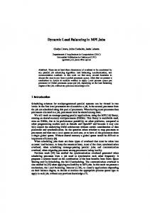
Fig. 1. Cutting planes (left) and associated cut tree (right) for recursive bisection. Dots are objects to be balanced; cuts are shown with colored lines and tree nodes.

traditional finite element methods (so much so that many application developers erroneously use the terms “graph partitioning” and “load balancing” interchangeably), geometric proximity of objects is more important than their graph connectivity in these applications. In crash simulations, for example, efficient parallel detection of contact surfaces can be achieved when physically close surfaces are grouped within processors [16]. While graph-based decompositions have been used in contact detection, they require construction of a geometric map for contact search [32]. Computing a parallel decomposition with respect to geometric coordinates is a more natural and straightforward approach. Similarly, greatest efficiency for particle methods is achieved when subdomains contain particles that are physically close to each other [4,16]. Indeed, particle methods do not have a natural graph connectivity, making graph partitioning difficult or impossible to apply. Moreover, frequent changes in proximity due to geometry deformation or particle movement require repartitioning strategies that are faster and more dynamic than graph partitioners. Geometric partitioning is an old, conceptually simple, but often overlooked technique for quickly and inexpensively generating decompositions. Using only the geometric coordinates of objects, these methods assign regions of space to processors so that the weight of objects in each region is equal. Zoltan includes geometric partitioners based on recursive bisection and space-filling curves. Recursive bisection (RB) [1–3] computes a cutting plane that divides a physical region into two subregions, each with half of the simulation’s work (see Figure 1). This cutting procedure is applied recursively to each subregion until the number of subregions equals the number of partitions desired. (The number of partitions need not be a power of two; adjusting the work percentage on each side of a cut allows any number of partitions.) Zoltan includes Recursive Coordinate Bisection (RCB) [1], which uses cutting planes orthogonal to coordinate axes, and Recursive Inertial Bisection (RIB) [2,3], which computes cuts orthogonal to principal inertial axes of the geometry. A space-filling curve (SFC) maps n-dimensional space to one dimension [33]. 5

4. Second intersection: white

3. Start of 2nd search

2. First intersection: blue 1. Start of 1st search

5. Start of 3rd search

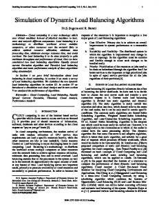
Fig. 2. SFC partitioning (left) and box-assignment search procedure (right). Dots (objects) are ordered along the red SFC. Partitions are indicated by color. The black box specified for box-assignment intersects the blue and white partitions.

In SFC partitioning, an object’s coordinates are converted to a SFC key representing the object’s position along a SFC through the physical domain. Sorting the keys gives a linear ordering of the objects (see Figure 2). This ordering is cut into appropriately weighted pieces that are assigned to processors. Zoltan method HSFC (Hilbert SFC) replaces the sort with adaptive binning [28]. Based upon their keys, objects are assigned to bins associated with partitions. Bin sizes are adjusted adaptively to obtain sufficient granularity for balancing. Geometric methods share many disadvantages and advantages. They are effective when only geometric locality is important and/or natural graph connectivity is not available. Because they do not explicitly control communication, geometric partitioners can induce higher communication costs than graph partitioners for some applications. However, because of their simplicity, they generally run faster and are easier to implement than graph partitioners. RCB and SFC partitioning are also implicitly incremental; that is, small changes in workloads tend to produce only small changes in the decomposition, resulting in little data movement between the old and new decompositions. This property is crucial in dynamic load balancing since the cost of moving application data is often high. Given the effectiveness of geometric methods for some applications, we present two enhancements that increase applicability of these algorithms: assignment for contact detection and multicriteria partitioning. Assignment for Contact Detection: In crash simulations, contact detection consists of finding all mesh points that intersect a given set of surfaces. Parallel contact detection is often done in two steps [16]: 1) assign each surface to the partitions whose subdomains intersect the surface, and 2) within each partition, find the points intersecting surfaces assigned in step 1. The key kernels of step 1 are identifying which partitions’ subdomains intersect a given point or region. We define these kernels as point-assignment and boxassignment, respectively. Given a point in space, point-assignment returns 6

the partition owning the region of space containing the point. Given an axisaligned region of space (defined by a 2D or 3D box), box-assignment returns a list of partitions whose assigned regions overlap the specified box; this box can be, say, a bounding box around a contact surface. Point- and box-assignment are implemented easily for RB methods [16]. The cutting planes used to generate a RB decomposition are stored as a binary tree, as shown in Figure 1. The root represents the plane dividing the initial geometry into two subregions; children represent planes cutting each of the subregions. Each leaf represents the partition to which a subregion is assigned. This tree describes the entire decomposition, yet is small enough to be stored on each processor, allowing point-assignment and box-assignment to be performed in serial. Using the cut tree, RB point-assignment determines on which side of the root cut the given point lies, and proceeds to the child subregion containing the point. Comparisons continue down the tree until a leaf is reached; the leaf’s partition is returned. For k partitions, RB point-assignment requires O(log k) operations. Similarly, in RB box-assignment, corners of the box are compared to the root cut. If any corner is less than the cut, the left child is visited; if any corner is greater than the cut, the right child is visited. Partitions associated with all leaves reached during the recursion are returned. RB box-assignment requires O(log k) operations in typical usage, and O(k) operations in the worst case (where every partition intersects the box). In Zoltan’s HSFC partitioning, point-assignment is also easily implemented. The k − 1 cuts dividing the SFC into k partitions describe the entire decomposition and can be stored on each processor. The SFC key for the given point is computed. A binary search for this key in the array of cuts returns the partition owning the space associated with key. Like RB point-assignment, SFC point-assignment requires O(log k) operations. Box-assignment, however, is difficult in SFC partitioning. Examination of the SFC cuts does not provide a description of the physical space assigned to each partition. Each entrance point of the SFC into the box must be found. Traversing the SFC is expensive and, unless done at extremely high resolution, could miss some partitions that lie within the box. We have developed an efficient box-assignment algorithm for SFC decompositions. Our implementation is strongly influenced by access of SFC-indexed databases in which high-dimensional SFCs are used to order database objects. The box-assignment problem is similar to the database problem of finding all data objects inside a specified box or all objects “near” a specified object in a database. Moore [34] developed software for several query methods (including variations of box-assignment) and fast conversion between Hilbert SFC keys 7

and spatial coordinates; his work was based on earlier work by Butz [35] and Thomas [36]. Lawder [37,38] presents a Hilbert-like SFC and practical conversions and spatial queries for high-dimensional database access; while his algorithms would work for a true Hilbert SFC, he created a Hilbert-like curve with more compact state tables necessary for high-dimensional databases. Our HSFC box-assignment algorithm calls a search routine, Next Query, that returns one intersecting partition per call. Starting with SFC key zero as input, Next Query returns the first partition m, 0 ≤ m < k, along the SFC that intersects the box. Then, starting at the SFC cut between partitions m and m+1, Next Query returns the next intersecting partition q, m+1 ≤ q < k. The search ends when no more partitions intersect the box. Thus, Next Query is called p + 1 times, where p is the number of partitions intersecting the box. An example is shown in Figure 2. Next Query recursively divides the spatial domain into octants and visits them in the order that the SFC enters them. The SFC value passed to Next Query represents the lowest SFC key assigned to the first partition m to check for intersection. Next Query finds the lowest numbered octant intersecting the box whose SFC key is not less than the input value. For each octant, it creates a partial SFC key by appending bits representing the octant’s position to bits from higher octree levels; this partial key represents the subtree rooted at the current octant. If the partial key is less than the input key, the subtree either is not in the box or is owned by partitions 0 to m − 1; no further search of the subtree is needed. Also, if the octant’s extent (computed from the partial key) does not intersect the box, the search continues to the next octant in the SFC. If, however, the extent intersects the box, the octant becomes the new spatial domain, the octant is refined, and the search is applied recursively to the octant’s children until the required SFC key resolution is reached. (Occasionally, a partial key does not provide enough resolution to rule out a subtree, even though the subtree does not meet the search criteria; in this case, stored backtracking information allows efficient restart.) The final computed SFC key is then the smallest not-previously-found SFC key intersecting the box. A binary search of the SFC cuts produces the partition in which the computed key lies. HSFC box-assignment requires O(p log k) operations. To convert SFC keys to coordinates efficiently, Next Query uses two transition tables [39]. These tables represent the SFC as an octree without explicitly constructing the octree. Given an octant and its orientation in the SFC (i.e., reflection and rotation of the Hilbert “U” curve), the data table returns bits indicating the x, y, and z positions of the octant within the orientation. These bits are concatenated through all levels of the octree and converted to floating point coordinates. Given an octant and its orientation, the state table returns the orientation of the SFC for the octant’s children. Inverse tables convert coordinates to SFC keys. This conversion can be thought of as numbering 8

octants in the order that the SFC enters them, selecting the octant containing the spatial point, and appending the octant’s number to the key. Example 1 We tested our HSFC box-assignment algorithm on a 1.04 millionelement mesh of a chemical reactor. We generated an initial decomposition (96 partitions on a 16-processor Compaq/DEC Alpha cluster at Sandia) using RCB or HSFC. We then perturbed the mesh coordinates (as in contact/deformation problems) and repartitioned using the same method. For each method, we did 10,000 box-assignments on each processor. The box size was the average element size, a typical size in contact detection. Box locations were chosen randomly. In Table 1, we show the maximum (over all processors) time and number of intersecting partitions for 10,000 box-assignments. Due to the less regular shape of HSFC subdomains, more intersecting partitions were found by HSFC box-assignment. The work needed for local contact search (step 2 above) is proportional to the number of intersecting partitions; however, the differences seen here do not raise concern. HSFC partitioning took less time than RCB partitioning, while HSFC box-assignment took more time than RCB box-assignment. Since box-assignment is typically done thousands of times per decomposition, the relative benefits of RCB and HSFC depend on the particular application and problem. However, for applications preferring HSFC decompositions, availability of HSFC box-assignment is a benefit. 2 Table 1 Results comparing RCB and HSFC box-assignment for Example 1. Partitioner

# of Intersecting Parts for 10,000 box-assignments

Partitioning Time

Time for 10,000 box-assignments

RCB

10,931

0.71 secs

0.027 secs

HSFC

10,983

0.59 secs

0.176 secs

Multicriteria Geometric Partitioning: Crash simulations are “multiphase” applications consisting of two separate phases: computation of forces and contact detection. Often, separate decompositions are used for each phase; data is communicated from one decomposition to the other between phases [16]. Obtaining a single decomposition that is good with respect to both phases would remove the need for communication between phases. Each object would have multiple loads, corresponding to its workload in each phase. The challenge would be computing a single decomposition that is balanced with respect to all loads. Such a multicriteria partitioner could be used in other situations as well, such as balancing both computational work and memory usage. Karypis et al. [21,32,40] have considered multicriteria graph partitioning and its use in crash simulations. However, since geometric partitioners are often preferred, we aim to enable geometric algorithms to balance multiple loads. Good solutions to the multicriteria partitioning problem may not exist for all problems with geometric methods; the best we can hope for are heuristics that 9

work well on many problems. We are not aware of previous efforts in this area. Most geometric partitioners reduce the partitioning problem to a one-dimensional problem. RCB, for example, bisects the geometry perpendicular to only one coordinate axis at a time; the corresponding coordinate of the objects defines a linear order. Thus, even if the original partitioning problem has objects in multidimensional space (typically R3 ), we restrict our attention to the one-dimensional partitioning problem. This problem is also known as chains-on-chains, and has been well studied for the single-load case [41–43]. Traditional optimization problems are written in the standard form: minimize f (x) subject to some constraints. Hence, handling multiple constraints is easy, but handling multiple objectives is much harder as it does not fit into this form. Multicriteria load balancing can be formulated as either a multiconstraint or multiobjective problem. Often, the balance of each load is considered a constraint and has to satisfy a certain tolerance. Such a formulation fits the standard form, where, in this case, there is no objective, only constraints. Unfortunately, there is no guarantee that a solution exists to this problem. In practice, we want a “best possible” decomposition, even if the desired balance criteria cannot be satisfied. Thus, an alternative is to make the constraints objectives; that is, we want to achieve as good balance as possible with respect to all loads. Multiobjective optimization is a very hard problem, because, in general, the objectives conflict and there is no unique “optimal solution.” In dynamic load balancing, speed is often more important than quality of the solution. The unicriterion (standard) RCB algorithm is fast because each bisecting cut can be computed very quickly. Computing the cuts is fast because it requires solving only a unimodal optimization problem. We want the same speed to apply in the multicriteria case. Thus, we can remove many methods from consideration because we cannot afford to solve a global optimization problem, not even in one dimension. We consider mathematical models of the multicriteria bisection problem. Although the partitioning problem allows for k partitions, we will focus on the bisection problem, i.e., k = 2. The solution for general k can be obtained by recursively bisecting the resulting partitions. Given a set of n points, let a1 , a2 , . . . , an be the corresponding loads (weights). Informally, our objective P P is to find an index s, 1 ≤ s ≤ n, such that i≤s ai ≈ i>s ai . When each ai is scalar, this problem is easy to solve. One can simply minimize the larger sum: min max( s

X i≤s

ai ,

X

ai ).

i>s

In the multicriteria case, however, each ai is a vector and the problem is not well-defined. In general, no index s achieves approximate equality in every 10

dimension. Applying the weighted sum method to the formula above yields min wT max( s

X i≤s

ai ,

X

ai ),

i>s

where the maximum of two vectors is defined element-wise and w is a cost vector, possibly all ones, that combines multiple objectives into a single objective. This formulation is reasonable for load balancing: assuming component j of ai represents the work associated with object i and phase j, we minimize the total time over all phases, where one phase cannot start before the previous one has finished. Unfortunately, it is hard to solve; because the function is non-convex, global optimization is required. Instead, we propose a heuristic: min max(g( s

X

ai ), g(

i≤s

X

ai )),

i>s

where g is a monotonically non-decreasing function in each component of the input vector. Motivated by the global criterion method, we suggest using P either g(x) = j xpj with p = 1 or p = 2, or g(x) = kxk for some norm. This formulation has one crucial computational advantage: the objective function is unimodal with respect to s. In other words, starting with s = 1 and increasing s, the objective decreases, until at some point the objective starts increasing. That point defines the optimal bisection value s. Note that the objective may be locally flat (constant), so there is not always a unique minimizer. While we did not explicitly scale the weights in our description above, scaling is important since our approach implicitly compares values corresponding to different weight dimensions. We implemented two types of scaling: no scaling or imbalance-tolerance scaling. No scaling is useful when the magnitude of the weights reflects the importance of the load types. But in general, the natural scaling is to make all weight dimensions equally important. To account for user-specified imbalance tolerances (i.e., amount of load imbalance allowed for each weight dimension), we scale the weights such that the load types with the largest imbalance tolerance have the smallest sum, and vice versa. Example 2 We present results using a 4000-element mesh of a chemical reactor with two weights per element (d = 2). For each element, the first weight is one; the second corresponds to the number of its faces having no face neighbors (i.e., on the external surface). This weighting scheme is realistic for contact problems. Tests were run on a Compaq/DEC Alpha cluster at Sandia. We divided this mesh into k = 9 partitions using our multicriteria RCB code and compared against ParMETIS. Results are shown in Table 2. BALAN CE[i] is the maximum processor load for weight i divided by the average processor load for weight i, i = 0, . . . , d−1. We observe little difference between the multicriteria RCB algorithms using different norms. The balances are not quite as good as ParMETIS, which was expected since the RCB cuts are restricted to orthogonal planes. Still, the multicriteria RCB algorithm produces reason11

able load balance for this problem in less time than ParMETIS and provides a viable alternative for applications lacking graph connectivity. For comparison, we include the results for RCB with d = 1; i.e., only the first weight is used. The edge cuts are the number of graph edges that are cut by partition boundaries, approximating communication volume in parallel applications. 2 Table 2 Results comparing multicriteria RCB and multicriteria ParMETIS for Example 2. k=9

RCB d=1

RCB d=2 norm=1

RCB d=2 norm=2

RCB d=2 norm=max

ParMETIS d=2

BALANCE[0]

1.00

1.13

1.13

1.12

1.01

1.11

1.11

1.16

1.01

BALANCE[1] Edge Cuts

1576

1502

1500

1468

1516

Time

0.10

0.11

0.12

0.11

0.25

While further experimentation is needed, initial results are promising. A natural question is how much better one can do by choosing an arbitrary cutting plane at every step. (RCB is restricted to cutting along coordinate axes.) There is an interesting theoretical result, known as the Ham Sandwich Theorem [44], which implies that a set of points in Rn , each with an n-dimensional binary weight vector, can be cut by a (n − 1)-dimensional hyperplane such that the vector sum in the two half-spaces differs by at most one in each vector component. A linear time algorithm exists for n = 2, and some efficient algorithms exist for other low dimensions [45].

4

Hypergraph Models

New simulation areas such as electrical systems, computational biology, linear programming and nanotechnology show the limitations of current partitioning technologies. Critical differences between these areas and more traditional mesh-based PDE simulations include high connectivity, heterogeneity in topology, and matrices that are rectangular or non-symmetric. The non-zero structure of the matrix in Table 4, taken from a density functional theory simulation of polymer self-assembly [46], is representative of these new applications; one can easily see the vastly different structure of this matrix compared to a traditional finite element matrix (Table 3). More robust partitioning models are needed for efficient parallelization of these applications. Graph models are often considered the most effective models for mesh-based PDE simulations. In graph models, graph vertices represent the data to be partitioned (e.g., elements, matrix rows). Edges represent relationships be12

A

A

Fig. 3. Example of communication metrics in graph (left) and hypergraph partitioning (right). Edges are shown in blue; the partition boundary is shown in red.

tween vertices (e.g., shared faces, off-diagonal matrix entries), The number of edges “cut” by a subdomain boundary (i.e., connecting vertices in different partitions) approximates the volume of communication needed during computation (e.g., flux calculations, matrix-vector multiplication). Vertices and edges can be weighted to reflect associated computation and communication costs, respectively. The goal of graph partitioning, then, is to assign equal total vertex weight to partitions while minimizing the weight of cut edges. It is important to note that the edge-cut metric is only an approximation of communication volume. For example, in Figure 3 (left), a grid is divided into two partitions (separated by a red line). Grid point A has four graph edges associated with it; each edge (shown in blue) connects A with a neighboring grid point. Two of the edges are cut by the partition boundary; however, the actual communication volume associated with sending A to the neighboring processor is only one grid point. Nonetheless, countless examples demonstrate the success of graph partitioning in sparse iterative solvers and mesh-based PDE applications; the approximation is often good enough for these applications. Another limitation of the graph model is the type of systems it can represent [47]. Because edges in the graph model are non-directional, they imply symmetry in all relationships, making them appropriate only for problems represented by square, symmetric matrices. Non-symmetric systems A must be represented by a symmetrized model A + AT , adding new edges to the graph and further skewing the communication metric. While a directed graph model could be adopted, it would not improve the communication metric’s accuracy. Likewise, graph models can not represent rectangular matrices, such as those arising in linear programming. Kolda and Hendrickson [48] propose using bipartite graphs. For an m × n matrix A, vertices mi , i = 1, . . . , m represent rows, and vertices nj , j = 1, . . . , n represent columns. Edges eij connecting mi and nj exist for non-zero matrix entries aij . But as in other graph models, the number of cut edges only approximates communication volume. Hypergraph models [49] address many of the drawbacks of graph models. As 13

in graph models, hypergraph vertices represent the work of a simulation. However, hypergraph edges (hyperedges) are sets of two or more related vertices. The number of hyperedge cuts is an exact representation of communication volume, not merely an approximation [49]. In the example in Figure 3 (right), a single hyperedge (shown in blue) including vertex A and its neighbors is associated with A; this single cut hyperedge accurately reflects the communication volume associated with A. Catalyurek and Aykanat [49] also describe the greater expressiveness of hypergraph models over graph models. Hypergraph models do not imply symmetry in relationships, allowing both non-symmetric and rectangular matrices to be represented. For example, the rows of a rectangular matrix could be represented by the vertices of a hypergraph. Each matrix column would be represented by a hyperedge connecting all non-zero rows in the column. Hypergraph partitioning’s effectiveness has been demonstrated in many areas, including VLSI layout [50], sparse matrix decompositions [49,51], and database storage and data mining [52,53]. Serial hypergraph partitioners are available (e.g., hMETIS [54], PaToH [49,55], Mondriaan [51]), but for large-scale and dynamic applications, parallel hypergraph partitioners are needed. As a precursor to parallel hypergraph partitioning, we have developed a serial hypergraph partitioner in Zoltan. Like other hypergraph partitioners [49,54,55], our hypergraph partitioner uses multi-level strategies developed for graph partitioners [10–12]. In the multi-level algorithm, we coarsen a hypergraph into successively smaller hypergraphs. We partition the smallest hypergraph and project the coarse decomposition back to the larger hypergraphs, using local optimization to reduce hyperedge cuts while maintaining balance at each level. The coarsening phase uses reduction methods that are based on graph matching algorithms adapted to hypergraphs. Each type of reduction method — matching, packing, and grouping — selects a set of vertices and combines them into a single, “larger” vertex. In matching, a pair of connected vertices is replaced with an equivalent vertex; the new vertex’s weight, connectivity, and associated hyperedge weights represent the original pair of vertices reasonably. Packing methods replace all vertices connected by a hyperedge with an equivalent vertex. Grouping methods replace all ungrouped vertices connected by a single hyperedge with an equivalent vertex. Optimal matching, packing and grouping algorithms are typically very time consuming; they either are NP-complete or have run-times that are O(np ) where p is large. Thus, we implemented several fast approximation algorithms for these tasks [56]. The coarsest hypergraph is then partitioned. If the coarsest hypergraph has k or fewer vertices (where k is the number of requested partitions), each vertex is trivially assigned to a partition. Otherwise, a greedy partitioning method 14

establishes the coarse-hypergraph decomposition. Finally, the coarse partition is projected onto the successively finer hypergraphs. A coarse vertex’s partition assignment is given to all fine vertices that were reduced into the coarse vertex. At each projection, a variation of the Fiduccia-Mattheyes [57] optimizer reduces the weight of cut hyperedges while maintaining load balance. The local optimizer generates two partitions (k = 2). For k > 2, the hypergraph partitioner is applied recursively. Example 3 To demonstrate the effectiveness of hypergraph partitioning, we applied both graph and hypergraph partitioners to matrices and compared the communication volume required for matrix-vector multiplication using the resulting decompositions. For both methods, each row i of the matrix A was represented by node ni . For hypergraph methods, each column j was represented by a hyperedge hj with hj = {ni : aij 6= 0}. For graph methods, edge eij connecting nodes ni and nj existed for each non-zero aij or aji in the matrix A; that is, the graph represented the symmetrized matrix A + AT . The first matrix is from a standard hexahedral finite element simulation; it is symmetric and very sparse. This type of matrix is represented well by graphs. As a result, hypergraph partitioning has only a small advantage over graph partitioning for this type of matrix [49]. For a five-partition decomposition, hypergraph partitioning reduced total communication volume 2-22% compared to graph partitioning. Detailed results are in Table 3; the “best” and “worst” Zoltan hypergraph methods correspond to different reduction strategies. Greater benefit from hypergraph partitioning is seen using a matrix from a polymer self-assembly simulation in the density-functional theory (DFT) code Tramonto [46]. The matrix has 46,176 rows with 3,690,048 non-zeros in an intricate sparsity pattern arising from the wide stencil used in Tramonto. For an eight-partition decomposition, hypergraph partitioning reduced total communication volume 37-56% relative to graph partitioning. Hypergraph partitioning also reduced the number of neighboring partitions. Detailed results are in Table 4. Because our methods are not yet optimized, we do not report partitioning times; however, Catalyurek and Aykanat show that hypergraph partitioning takes up to 2.5 times as much time as graph partitioning [49]. 2 These experiments and others [49] show the promise of hypergraph partitioning for emerging applications. To be effective for dynamic load balancing, however, parallel hypergraph partitioners are needed. Also, to keep data movement costs low, incremental hypergraph algorithms are needed; extension of diffusive graph algorithms [13] to hypergraphs is a logical approach, but is complicated by the hyperedges’ larger cardinality. 15

Table 3 Comparison of graph and hypergraph partitioning for HexFEM matrix (Example 3). HexFEM Matrix: • Hexahedral 3D structured-mesh finite element method. • 32,768 rows • 830,584 non-zeros • Five partitions Partitioning Method

Imbalance (Max / Avg Work)

# of Neighbor Partitions per Partition

Communication Volume over all Partitions

Max

Avg

Max

Total

Reduction of Total Communication Volume

Graph method (METIS PartKWay)

1.03

4

3.6

1659

6790

Best Zoltan hypergraph method (RRM)

1.013

4

3.6

1164

5270

22%

Worst Zoltan hypergraph method (RHP)

1.019

4

2.8

2209

6644

2%

Table 4 Comparison of graph and hypergraph partitioning for PolyDFT matrix (Example 3). PolyDFT matrix • Polymer self-assembly simulation • Density functional theory code • 46,176 rows • 3,690,048 non-zeros • Eight partitions Partitioning Method

Imbalance (Max / Avg Work)

# of Neighbor Partitions per Partition

Communication Volume over all Partitions

Max

Avg

Max

Total

Reduction of Total Communication Volume

Graph method (METIS PartKWay)

1.03

7

6

7382

44,994

Best Zoltan hypergraph method (MXG)

1.018

5

4

3493

19,427

56%

Worst Zoltan hypergraph method (GRP)

1.03

6

5.25

5193

28,067

37%

16

5

Resource-Aware Load Balancing

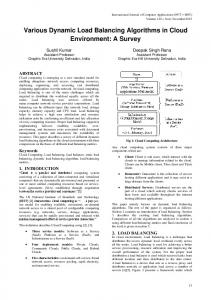
Load-balancing research is driven not only by emerging applications, but also by emerging parallel architectures. These new architectures span many scales. Clusters have become viable alternatives to tightly coupled parallel computers for small-scale systems. They are cost-effective environments for running computationally intensive distributed applications. An attractive feature of clusters is the ability to increase their computational power by adding nodes. Such expansions can result in heterogeneous environments, as newly added nodes often have superior capabilities. On the medium scale, many supercomputers (e.g., ASCI Q, Earth Simulator) are constructed as networks of shared-memory multiprocessors (SMPs) with complex and non-homogeneous interconnection topologies. And on the largest scale, grid technologies have enabled computation on widely distributed systems, combining geographically distributed clusters and supercomputers into a single computational resource. These grids introduce extreme computational and network heterogeneity. To distribute data from any application effectively on such systems, partitioners must be resource-aware; that is, they must account for heterogeneity in the execution environment. Resource-aware balancing requires gathering information about the computing environment (e.g., computing, network and memory availability), and determining how to use the information for load balancing (e.g., by adjusting partition sizes and/or selecting appropriate partitioning algorithms). A number of projects attempt to address these issues. Teresco et al. [58] use a directed-graph model to represent hierarchical environments; their work is a precursor of the work described here. Minyard and Kallinderis [59] monitor process “wait times” to assign element weights that are used in octree partitioning. Walshaw and Cross [60] couple a multilevel graph algorithm with a model of a heterogeneous communication network to minimize a communication cost function. Sinha and Parashar [61] use the Network Weather Service (NWS) [62] to gather information about the state and capabilities of available resources; they compute the load capacity of each node as a weighted sum of processing, memory, and communications capabilities. We are developing a model for resource-aware load balancing called DRUM (Dynamic Resource Utilization Model) [63]. DRUM provides applications aggregated information about the computation and communication capabilities of an execution environment. DRUM can be viewed as an abstract object that 1) encapsulates the details of hardware resources, capabilities and interconnection topology, 2) provides a facility for dynamic, modular, and minimally intrusive monitoring of an execution environment, and 3) distills this information to a scalar “power” value, readily usable by any load-balancing algorithm as the percentage of overall application load to be assigned to a partition. DRUM has been designed to work with Zoltan, but may also be used as a 17

separate library. DRUM represents the underlying interconnection network topology of hierarchical systems (e.g., clusters of clusters, or clusters of multiprocessors) as a tree. The root of the tree represents the total execution environment. Its children are high-level divisions of networks connected to form the total execution environment. Sub-environments are recursively divided, according to the network hierarchy, with the tree leaves being individual computation nodes (i.e., single processors (SP) or SMPs). Computation nodes have data representing their relative computing and communication power. Non-leaf network nodes, representing routers or switches, have an aggregate power calculated as a function of the powers of their children and the network characteristics. In Figure 4, we show a tree representing a cluster with eight SPs and three SMPs connected in a hierarchical network structure. Communication node

Processing node

Router

Router

Router

Router

SP

SMP

Switch

SMP

SMP

SP

SP

SP

SP

SP

SP

SP

Fig. 4. Tree constructed by DRUM to represent a heterogeneous network.

Necessary knowledge of the execution environment’s underlying topology is specified in an XML file created by running a graphical configuration tool. The configuration tool also assesses nodes’ computational capabilities by running benchmarks (currently LINPACK [64]) and checks for optional facilities used by DRUM (e.g., threading capabilities). The configuration tool needs to be re-run only when hardware characteristics of the system have changed. Powers may be computed from the static benchmark data only or may include dynamic information from monitoring agents. At every node, agents in separate threads probe network interfaces for communication volume; network nodes are monitored by representative processes. At each computation node, agents measure the CPU load and memory capacity as viewed by each local process of the parallel job. (An NWS interface is also available for gathering this information.) We compute the power of node n as the weighted sum of a processing power pn and a communication power cn : powern = wncomm cn + wncpu pn ,

wncomm + wncpu = 1.

Since multiple relevant processes might run on each node n, we extend the no18

tion of a node’s power to processes. We denote LP n = {psn,j , j = 1, 2, . . . , kn }, the set of kn processes psn,j running on node n and invoking DRUM services. For computation node n with m CPUs, we evaluate the processing power pn,j for each process psn,j in LP n based on (i) CPU utilization un,j by process psn,j , (ii) the percentage it of time that CPU t is idle (and, thus, available for computation if processes receive more work), and (iii) the node’s static P benchmark rating (in MFLOPS) bn . The overall idle time in node n is m t=1 it . However, when kn < m, the maximum exploitable total idle time is kn − Pk n j=1 un,j . Therefore, the total idle time that processes ps n,j could exploit is P n P min(kn − kj=1 un,j , m t=1 it ). Assuming all processes psn,j on node n should have equal power, we compute average CPU usage and idle times per process: kn kn m X X 1 X 1 it ) . un,j , in = un,j , un = min(kn − kn j=1 kn t=1 j=1

Processing power pn,j is estimated as pn,j = bn (un + in ), j = 1, 2, . . . , kn . n Since pn,j is the same for all processes j on node n, pn = kj=1 pn,j = kn pn,1 . On internal nodes, pn is the sum of the processing powers of the nodes’ children.

P

We estimate a node’s communication power based on the communication traffic at the node. At each computation and (when possible) network node, agents estimate the average rate of incoming packets λ and outgoing packets µ on each relevant communication interface. We view a node’s communication power as inversely proportional to the communication activity factor CAF = λ + µ at that node. The CAF provides dynamic information about the traffic passing through a node, the communication traffic at neighboring nodes, and, to some extent, the traffic in the overall system. The communication power of nodes with more than one interface (e.g., routers) is computed as the average of the powers on each interface. Let CAFn,i denote the CAF of interface i of a node n with s interfaces. We estimate the communication power as s 1 1X cn = . s i=1 CAFn,i

In practice, software loop-back interfaces and interfaces with CAF = 0 are ignored. To compute per-process communication powers for processes j, j = 1, 2, . . . , kn , on node n, we compute cn and associate k1n cn with each process. For consistency, if at least one non-root network node cannot be probed for communication traffic, all internal nodes are assigned CAF values computed as the sum of their immediate children’s values. The value of wncomm is currently specified manually. The possibility of basing wncomm on dynamic factors, such as CAF , is being considered. 19

A top-down normalization is also performed for the values of pn and cn at each level of the tree. Thus, for each node n in Li (the set of nodes at level i), the final power is computed as cn powern = ppn (wncomm P|Li |

j=1 cj

pn + wncpu P|Li |

j=1 pj

)

where ppn is the power of the parent of node n; for the root node, ppn = 1. Example 4 We present experimental results using DRUM in the solution of a Laplace equation on the unit square, using Mitchell’s Parallel Hierarchical Adaptive MultiLevel software (PHAML) [65]. After 17 adaptive refinement steps, the mesh has 524,500 nodes. We used a Sun cluster at Williams College consisting of “fast” 450MHz Sparc UltraII nodes and “slow” 300/333MHz Sparc UltraII processors, connected by fast (100 Mbit) Ethernet. Benchmark runs indicated that the fast nodes have a computation rate of approximately 1.5 times faster than the slow nodes. Given an equal distribution of work, the fast nodes would be idle one third of the time. Zoltan’s HSFC procedure is used for partitioning; results are similar for other methods. Table 5 shows wall clock solution times using equally sized partitions and DRUM’s resource-aware partitions. Computations on uniform speed processors indicate only a small overhead incurred by DRUM’s dynamic monitoring. With uniform partitions, adding two slow processors actually slows the computation. DRUM’s resource-aware partitions allow more effective use of these processors, particularly when factoring in communication power. In preliminary experiments with larger numbers of processors, DRUM’s resource-aware partitions show similar improvements. 2 Table 5 Solution wall clock times (in seconds) using uniformly sized partitions and DRUM’s resource-aware partitions for various values of wncomm in Example 4. Nodes

Uniform

wncomm = 0.0

wncomm = 0.1

wncomm = 0.25

4 fast

292.33

295.53

294.94

295.04

4 fast+2 slow

348.35

270.23

263.11

283.05

4 fast+4 slow

268.03

248.20

243.48

235.02

Many enhancements to DRUM are underway or planned for the future. The expression for the communication power is being revised to include information such as interface speed (bandwidth) and link latency. Dynamic communication weight selection is being investigated. When communication is overlapped with computation, a weighted sum may not be an accurate model, so other ways to combine communication and processing power will be considered. We are also investigating ways to include memory statistics into the power expression. DRUM agents currently monitor the available and total memory on 20

each computation node. More refined memory statistics (e.g., number of cache levels, cache hit ratio, cache and main memory access times) are needed to capture memory effects in the model. We are also developing a package for data collection and analysis that will enable us to filter noisy data and obtain better estimates of computational and communication performance. Most previous work focuses on incorporating environment information into pre-selected partitioning algorithms. As an alternative, such information could be used to select appropriate partitioning strategies. For example, DRUM’s hierarchical machine model leads naturally to topology-driven hierarchical partitioning. Work is divided among the children of the root of the DRUM tree, with the child nodes’ powers determining the amount of work to be assigned to each node. The work assigned to these nodes is then recursively partitioned among the nodes in their subtrees. Different partitioning methods can be used in each level and subtree to produce effective partitions with respect to the network; for example, graph or hypergraph partitioners could minimize communication between nodes connected by slow networks while fast geometric partitioners operate within each node. We are developing these capabilities in Zoltan. Preliminary tests use an adaptive finite element simulation on a Sun cluster of multiprocessors. The subsets of the cluster used for the experiments are four two-processor 450MHz Sparc UltraII nodes and two four-processor 450MHz Sparc UltraII nodes, all connected by fast (100 Mbit) Ethernet. Among all combinations of traditional and hierarchical procedures, time to solution was often minimized using hierarchical load balancing using ParMETIS for inter-node partitioning and RIB within each node [66]. Further studies will be performed using hierarchical balancing on larger clusters and with a wider variety of architectures and applications.

6

Conclusions and Future work

While great progress has been made in dynamic load balancing for parallel, unstructured and/or adaptive applications, research continues to address issues arising due to application and architecture requirements. Existing algorithms, such as the geometric algorithms RCB and HSFC, are being augmented to support special needs of complex applications. New models using hypergraphs are being developed to more accurately represent highly connected, non-symmetric, and/or rectangular systems arising in density functional theory, circuit simulations, and integer programming. On heterogeneous computer architectures, software such as DRUM dynamically detects the available computing, memory and network resources, and provides the resource information to both existing partitioning algorithms and new hierarchical partitioning strategies. Software toolkits such as Zoltan deliver these capabilities 21

to applications, enable comparisons of methods within applications, and serve as test-beds for further research and development. While we present some solutions to these issues, our work represents only a small sample of continuing research into load balancing. For adaptive finite element methods, data movement from an old decomposition to a new one can consume orders of magnitude more time than the actual computation of a new decomposition; highly incremental partitioning strategies that minimize data movement are important for high performance of adaptive simulations [67,68]. In overlapping Schwartz preconditioning, the work to be balanced depends on data in both the processor’s subdomain and the overlap region, while the size of the overlap region depends on the subdomain generated by the partitioner. In such cases, standard partitioning models that assume work per processor is the total weight of objects assigned to the processor are insufficient; strategies that treat workloads as a function of the subdomain are needed [69]. Very largescale semantic networks place additional demands on partitioners, due to both their high connectivity and irregular structure; highly effective partitioning techniques for these networks are in their infancy [70]. These examples of research in partitioning, while still not exhaustive, demonstrate that, indeed, the load-balancing problem is not yet solved.

References [1] M. J. Berger, S. H. Bokhari, A partitioning strategy for nonuniform problems on multiprocessors, IEEE Trans. Computers C-36 (5) (1987) 570–580. [2] H. D. Simon, Partitioning of unstructured problems for parallel processing, in: Proc. Conference on Parallel Methods on Large Scale Structural Analysis and Physics Applications, Pergammon Press, 1991. [3] V. E. Taylor, B. Nour-Omid, A study of the factorization fill-in for a parallel implementation of the finite element method, Int. J. Numer. Meth. Engng. 37 (1994) 3809–3823. [4] M. S. Warren, J. K. Salmon, A parallel hashed oct-tree n-body algorithm, in: Proc. Supercomputing ’93, Portland, OR, 1993. [5] J. R. Pilkington, S. B. Baden, Partitioning with spacefilling curves, CSE Technical Report CS94–349, Dept. Computer Science and Engineering, University of California, San Diego, CA (1994). [6] A. Patra, J. T. Oden, Problem decomposition strategies for adaptive hp finite element methods, Computing Systems in Engg. 6 (2) (1995) 97–109. [7] W. F. Mitchell, Refinement tree based partitioning for adaptive grids, in: Proc. Seventh SIAM Conf. on Parallel Processing for Scientific Computing, SIAM, 1995, pp. 587–592.

22

[8] J. Flaherty, R. Loy, M. Shephard, B. Szymanski, J. Teresco, L. Ziantz, Adaptive local refinement with octree load-balancing for the parallel solution of threedimensional conservation laws, J. Parallel Distrib. Comput. 47 (2) (1998) 139– 152. [9] A. Pothen, H. Simon, K. Liou, Partitioning sparse matrices with eigenvectors of graphs, SIAM J. Matrix Anal. 11 (3) (1990) 430–452. [10] T. Bui, C. Jones, A heuristic for reducing fill in sparse matrix factorization, in: Proc. 6th SIAM Conf. Parallel Processing for Scientific Computing, SIAM, 1993, pp. 445–452. [11] B. Hendrickson, R. Leland, A multilevel algorithm for partitioning graphs, in: Proc. Supercomputing ’95, ACM, 1995. [12] G. Karypis, V. Kumar, A fast and high quality multilevel scheme for partitioning irregular graphs, Tech. Rep. CORR 95–035, University of Minnesota, Dept. Computer Science, Minneapolis, MN (June 1995). [13] G. Cybenko, Dynamic load balancing for distributed memory multiprocessors, J. Parallel Distrib. Comput. 7 (1989) 279–301. [14] Y. Hu, R. Blake, An optimal dynamic load balancing algorithm, Tech. Report DL-P-95-011, Daresbury Laboratory, Warrington, WA4 4AD, UK (Dec. 1995). [15] E. Leiss, H. Reddy, Distributed load balancing: design and performance analysis, W.M. Keck Research Computation Laboratory 5 (1989) 205–270. [16] S. Plimpton, S. Attaway, B. Hendrickson, J. Swegle, C. Vaughan, D. Gardner, Transient dynamics simulations: Parallel algorithms for contact detection and smoothed particle hydrodynamics, J. Parallel Distrib. Comput. 50 (1998) 104– 122. [17] H. C. Edwards, A Parallel Infrastructure for Scalable Adaptive Finite Element Methods and its Application to Least Squares C ∞ Collocation, Ph.D. thesis, The University of Texas at Austin (May 1997). [18] K. Devine, J. Flaherty, Parallel adaptive hp-refinement techniques for conservation laws, Appl. Numer. Math. 20 (1996) 367–386. [19] K. Schloegel, G. Karypis, V. Kumar, Multilevel diffusion algorithms for repartitioning of adaptive meshes, Journal of Parallel and Distributed Computing 47 (2) (1997) 109–124. [20] C. Walshaw, M. Cross, K. McManus, Multiphase mesh partitioning, App. Math. Modelling 25 (2000) 123–140. [21] K. Schloegel, G. Karypis, V. Kumar, Parallel static and dynamic multiconstraint graph partitioning, Concurrency and Computation – Practice and Experience 14 (3) (2002) 219–240. [22] B. Hendrickson, R. Leland, The Chaco user’s guide, version 2.0, Tech. Rep. SAND94–2692, Sandia National Laboratories, Albuquerque, NM (Oct. 1994).

23

[23] C. Walshaw, The Parallel JOSTLE Library User’s Guide, Version 3.0, University of Greenwich, London, UK (2002). [24] R. Preis, R. Diekmann, The PARTY partitioning library, user guide version 1.1, Tech. Rep. tr-rsfb-96-024, Dept. of Computer Science, University of Paderborn, Paderborn, Germany (Sept. 1996). [25] F. Pelligrini, SCOTCH 3.4 user’s guide, Research Rep. RR-1264-01, LaBRI (Nov. 2001). [26] G. Karypis, V. Kumar, ParMETIS: Parallel graph partitioning and sparse matrix ordering library, Tech. Rep. 97-060, Department of Computer Science, University of Minnesota, available on the WWW at URL http://www.cs.umn.edu/~metis (1997). [27] K. Devine, E. Boman, R. Heaphy, B. Hendrickson, C. Vaughan, Zoltan data management services for parallel dynamic applications, Computing in Science and Engineering 4 (2) (2002) 90–97. [28] K. Devine, B. Hendrickson, E. Boman, M. St. John, C. Vaughan, Zoltan: A Dynamic Load Balancing Library for Parallel Applications; User’s Guide, Sandia National Laboratories, Albuquerque, NM, tech. Report SAND99-1377 http://www.cs.sandia.gov/Zoltan/ug_html/ug.html (1999). [29] K. D. Devine, B. A. Hendrickson, Tinkertoy parallel programming: A case study with Zoltan, Int. J. Computational Science and Engineering To appear. [30] B. Maerten, D. Roose, A. Basermann, J. Fingberg, G. Lonsdale, DRAMA: A library for parallel dynamic load balancing of finite element applications, in: Proc. Ninth SIAM Conference on Parallel Processing for Scientific Computing, San Antonio, TX, 1999. [31] A. Pinar, B. Hendrickson, Communication support for adaptive computation, in: Proc. 10th SIAM Conf. Parallel Processing for Scientific Computing, Portsmouth, VA, 2001. [32] G. Karypis, Multi-constraint mesh partitioning for computations, in: Proc. SC2003, ACM, Phoenix, AZ, 2003.

contact/impact

[33] H. Sagan, Space-Filling Curves, Springer-Verlag, New York, NY, 1994. [34] D. Moore, Fast hilbert curve generation, sorting and range queries, http:// www.caam.rice.edu/~dougm/twiddle/Hilbert. [35] A. Butz, Alternative algorithm for Hilbert’s space-filling curve, IEEE Trans. Comp. (1971) 424–426. [36] S. Thomas, Software Library, http://www.mit.edu/afs/athena.mit.edu/ activity/c/cgs/src/urt3.1/lib/hil%bert.c (1991). [37] J. Lawder, P. King, Using space-filling curves for multi-dimensional indexing, Lecture Notes in Computer Science 1832.

24

[38] J. Lawder, P. King, Querying multi-dimensional data indexed using the Hilbert space-filling curve, SIGMOD Record 30 (1) (2001) 19–24. [39] P. M. Campbell, The performance of an octree load balancer for parallel adaptive finite element computation, Master’s thesis, Computer Science Dept., Rensselaer Polytechnic Institute, Troy, NY (2001). [40] G. Karypis, V. Kumar, Multilevel algorithms for multiconstraint graph paritioning, Tech. Rep. 98-019, Department of Computer Science, University of Minnesota (1998). [41] M. A. Iqbal, Approximate algorithms for partitioning and assignment problems, Int. J. Parallel Programming 20 (5) (1991) 341–361. [42] B. Olstad, F. Manne, Efficient partitioning of sequences, IEEE Trans. Comp. 44 (1995) 1322–1326. [43] A. Pinar, Combinatorial algorithms in scientific computing, Ph.D. thesis, University of Illinois–Urbana-Champaign (2001). [44] A. H. Stone, J. W. Tukey, Generalized sandwich theorems, Duke Math. J. 9 (1942) 356–359. [45] C. Y. Lo, J. Matousek, W. Steiger, Algorithms for ham-sandwich cut, Disc. Comput. Geometry 11 (4) (1994) 433–452. [46] L. J. D. Frink, A. G. Salinger, M. P. Sears, J. D. Weinhold, A. L. Frischknecht, Numerical challenges in the application of density functional theory to biology and nanotechnology, J. Phys. Cond. Matter 14 (2002) 12167–12187. [47] B. Hendrickson, Graph partitioning and parallel solvers: Has the emperor no clothes?, Lecture Notes in Computer Science 1457 (1998) 218 – 225. [48] B. Hendrickson, T. Kolda, Graph partitioning models for parallel computing, Parallel Computing 26 (2000) 1519 – 1534. [49] U. Catalyurek, C. Aykanat, Hypergraph-partitioning based decomposition for parallel sparse-matrix vector multiplication, IEEE Trans. Parallel Dist. Systems 10 (7) (1999) 673–693. [50] A. Caldwell, A. Kahng, J. Markov, Design and implementation of move-based heuristics for VLSI partitioning, ACM J. Experimental Algs. 5 (5). [51] B. Vastenhouw, R. H. Bisseling, A two-dimensional data distribution method for parallel sparse matrix-vector multiplication, SIAM Review To appear. [52] C. Chang, T. Kurc, A. Sussman, U. Catalyurek, J. Saltz, A hypergraph-based workload partitioning strategy for parallel data aggregation, in: Proc. of 11th SIAM Conf. Parallel Processing for Scientific Computing, SIAM, 2001. [53] M. Ozdal, C. Aykanat, Hypergraph models and algorithms for data-pattern based clustering, Data Mining and Knowledge Discovery 9 (1) (2004) 29–57.

25

[54] G. Karypis, R. Aggarwal, V. Kumar, S. Shekhar, Multilevel hypergraph partitioning: application in VLSI domain, in: Proc. 34th conf. Design automation, ACM, 1997, pp. 526 – 529. [55] U. Catalyurek, C. Aykanat, Decomposing irregularly sparse matrices for parallel matrix-vector multiplications, Lecture Notes in Computer Science 1117 (1996) 75 – 86. [56] E. Boman, K. Devine, R. Heaphy, B. Hendrickson, M. Heroux, R. Preis, LDRD report: Parallel repartitioning for optimal solver performance, Tech. Rep. SAND2004–0365, Sandia National Laboratories, Albuquerque, NM (Feb. 2004). [57] C. M. Fiduccia, R. M. Mattheyses, A linear time heuristic for improving network partitions, in: Proc. 19th IEEE Design Automation Conf., IEEE, 1982, pp. 175– 181. [58] J. D. Teresco, M. W. Beall, J. E. Flaherty, M. S. Shephard, A hierarchical partition model for adaptive finite element computation, Comput. Methods Appl. Mech. Engrg. 184 (2000) 269–285. [59] T. Minyard, Y. Kallinderis, Parallel load balancing for dynamic execution environments, Comput. Methods Appl. Mech. Engrg. 189 (4) (2000) 1295–1309. [60] C. Walshaw, M. Cross, Multilevel Mesh Partitioning for Heterogeneous Communication Networks, Future Generation Comput. Syst. 17 (5) (2001) 601– 623, (originally published as Univ. Greenwich Tech. Rep. 00/IM/57). [61] S. Sinha, M. Parashar, Adaptive system partitioning of AMR applications on heterogeneous clusters, Cluster Computing 5 (4) (2002) 343–352. [62] R. Wolski, N. T. Spring, J. Hayes, The Network Weather Service: A distributed resource performance forecasting service for metacomputing, Future Generation Comput. Syst. 15 (5-6) (1999) 757–768. [63] J. Faik, L. G. Gervasio, J. E. Flaherty, J. Chang, J. D. Teresco, E. G. Boman, K. D. Devine, A model for resource-aware load balancing on heterogeneous clusters, Tech. Rep. CS-03-03, Williams College Department of Computer Science, http://www.cs.williams.edu/drum/ (2003). [64] J. J. Dongarra, C. B. Moler, J. R. Bunch, G. W. Stewart, LINPACK User’s Guide, SIAM, Philadelphia (1979). [65] W. F. Mitchell, The design of a parallel adaptive multi-level code in Fortran 90, in: Proc. 2002 Internatl. Conf. on Computational Science, Amsterdam, 2002. [66] J. D. Teresco, Hierarchical partitioning and dynamic load balancing for scientific computation, Tech. Rep. CS-04-04, Williams College Department of Computer Science, submitted as extended abstract to PARA ’04. (2004). [67] M. Berzins, A new algorithm for adaptive load balancing, in: Proc. of 12th SIAM Conf. Parallel Processing for Scientific Computing, SIAM, 2004.

26

[68] Y. F. Hu, R. J. Blake, D. R. Emerson, An optimal migration algorithm for dynamic load balancing, Concurrency: Prac. and Exper. 10 (1998) 467–483. [69] A. Pinar, B. Hendrickson, Exploiting flexibly assignable work to improve load balance, in: Proc. 14th ACM symp. Parallel algs and archs, ACM, 2002, pp. 155 – 163. [70] T. Eliassi-Rad, A. Pothen, A. Pinar, K. Henderson, E. Chow, B. Hendrickson, Graph partitioning for complex networks, in: Proc. of 12th SIAM Conf. Parallel Processing for Scientific Computing, SIAM, 2004.

27