chronous Parallel architecture model (BSP), which describes supersteps of com- ... Our parallel MD implementation is not bound to the limitations of the BSP ...
Modeling Dynamic Load Balancing in Molecular Dynamics to Achieve Scalable Parallel Execution ? Lars Nyland,1 Jan Prins,1 Ru Huai Yun,2 Jan Hermans,2 Hye-Chung Kum,1 and Lei Wang1 1
Computer Science Department, Univ. of North Carolina, Chapel Hill, NC 27599 http://www.cs.unc.edu/ 2 Biochemistry and Biophysics Department, Univ. of North Carolina, Chapel Hill, NC 27599 http://femto.med.unc.edu/
Abstract. To achieve scalable parallel performance in Molecular Dynamics Simulation, we have modeled and implemented several dynamic spatial domain decomposition algorithms. The modeling is based upon Valiant’s Bulk Synchronous Parallel architecture model (BSP), which describes supersteps of computation, communication, and synchronization. We have developed prototypes that estimate the differing costs of several spatial decomposition algorithms using the BSP model. Our parallel MD implementation is not bound to the limitations of the BSP model, allowing us to extend the spatial decomposition algorithm. For an initial decomposition, we use one of the successful decomposition strategies from the BSP study, and then subsequently use performance data to adjust the decomposition, dynamically improving the load balance. We report our results here.
1 Introduction A driving goal of our research group is to develop a high performance MD simulator to support biochemists in their research. Our goals are to study large timescale behavior of molecules and to facilitate interactive simulations [7]. Two main characteristics of the problem impede our goal: first is the large number of interactions in solvated biomolecules, and second is the small timestep that is required to adequately capture high frequency motions. To meet our goal, we must develop a parallel implementation that scales well even on small problem sizes. Because the communication cost, memory reference and load balance across processors trade in a complex fashion, we have analyzed candidate implementations using the BSP [10, 1] model. The most promising implementation was implemented and improved outside of the constraints of the BSP model. ? This work has been supported in part by the National Institutes of Health’s National Center
for Research Resources (grant RR08102 to the UNC/Duke/NYU Computational Structural Biology Resource).
At each step in MD simulation, the sum of all forces on each atom is calculated and used to update the positions and velocities of each atom. The bonded forces seek to maintain bond lengths, bond angles, and dihedral angles on single bonds, two-bond chains and three-bond chains, respectively. Non-bonded forces are comprised of the electrostatic forces and the Van der Waals forces. A cutoff radius is introduced to limit non-bonded atom interactions to pairs closer than a preset radius, R . This is still the most time-consuming portion of each step, even though the cutoff radius reduces the O(n2 ) work to O(n). The remaining longerrange forces are calculated by some other method [2, 5], calculated less frequently, or completely ignored. Good opportunities for parallelization in MD exist; all of the forces on each of the atoms are independent, so they can be computed in parallel. Once computed, the nonbonded forces are summed and applied in parallel. Good efficiency depends on good load-balancing, low overhead, and low communication requirements. Using a spatial decomposition increases data coherence, reducing communication costs. Two nearby atoms interact with all atoms that are within R of both, providing two opportunities for reduced communication. First, the atoms are near each other, thus accessing the data for many nearby atoms data will not require interprocessor communication. Second, for those interactions that require data from neighboring regions, atomic data can be fetched once and then reused many times, due to the similarities of interactions of nearby atoms. The use of a spatial decomposition for MD has become widespread in recent years. It is used by AMBER [3, 9], Charmm [6], Gromos [4] and NAMD [8], all of which run in a message-passing paradigm, as opposed to our shared-memory implementation. In general, each of these implementations found good scaling properties, but it is difficult to compare overall performance of the parallel MD simulators, as machine speeds have improved significantly since publication of the cited reports. Compared with these other implementations, our shared-memory implementation allows very precise loadbalancing on small systems.
2 Modeling Parallel Computation with the BSP Model The Bulk Synchronous Parallel (BSP) model has been proposed by Valiant [10] as a model for general-purpose parallel computation. It was further modified in [1] to provide a normalized cost of parallel algorithms, enabling uniform comparison of algorithms. The BSP model is both simple enough to quickly understand and use, but realistic enough to achieve meaningful results for many parallel computers. A parallel computer that is consistent with BSP architecture has a set of processormemory pairs, a communication network that transmits values in a point-to-point manner, and a mechanism for efficient barrier synchronization of the processors. Parallel computers are parameterized with 4 values: 1. The number of processors, P . 2. The processor speed, s, measured in floating-point operations per second. 3. The latency, L, which reflects the minimum latency to send a packet through the network, which also defines the minimum time to perform global synchronization.
4. The gap, g , reflecting the network communication bandwidth on a per-processor basis, measured in floating-point operation cycles taken per floating-point value sent. An algorithm for the BSP is written in terms of S supersteps, where a single superstep consists of some local computation, external communication, and global synchronization. The values communicated are not available for use until after the synchronization. The cost of the ith superstep is Ci = wi + ghi + L where wi is the maximum number of local operations executed by any processor and hi is the maximum number of values sent or received by any processor. The total cost of executing a program of S steps is then: C
tot
=
XS i=1
C
i
=
W
+ H g + S L;
where W
=
XS i=1
i and H
w
=
XS i=1
h
i
The normalized cost is the ratio between the BSP cost using P processors and the optimal work perfectly distributed over P processors. The optimal work, Wopt , is defined by the best known sequential algorithm. The normalized time is expressed as C (P )
The normalized cost can be reformulated as C (P ) = a + bg + L, where a = P � W=(Wopt ), b = P � H=(Wopt ), and = P � S=(Wopt ). When the triplet (a; b; ) = (1, 0, 0), the parallelization is optimal. Values where a > 1 indicate extra work is introduced in the parallelization and/or load imbalance among the processors. Values of b > 1=g or > 1=L indicate that the algorithm is communication bound, for the architecture described by particular values of g and L.
=
P
�
tot opt
C
W
for t = 1 to T by k { if Processor == 0 distribute atoms to processors calculate local pairlist for s = t to t+k - 1 { get remote atom information synchronize calculate forces on local atoms apply forces to update local positions/velocities } }
Fig. 1. A high-level, multiple timestep algorithm for performing parallel molecular dynamics computations (k small timesteps per large timestep).
3 BSP Modeling of Parallel MD In this section, we model several domain decompositions for MD simulation. We describe a simplified MD algorithm, the domain decompositions, and show the results of modeling. 3.1 A Simplified MD Algorithm The most time-consuming step of MD simulations is the calculation of the nonbonded forces, typically exceeding 90% of the execution time, thus we limit our modeling study to this aspect. Our simplified algorithm for computing the non-bonded forces
is shown in figure 1. It consists of an outer loop that updates the pairlist every k steps, with an inner loop to perform the force computations and application. The value k ranges from 10 to 50 steps, and is often referred to as the pairlist calculation frequency. In our modeling of MD, Molecular Input Data Name Atoms Name Atoms Name Atoms we examine the cost of exAlanine 66 Water 798 Eglin 7065 ecuting k steps to amortize Dipeptide (wet) 231 Argon 1728 Water 8640 the cost of pairlist calculaSS Corin 439 SS Corin (wet) 3913 Polio (segment) 49144 tion. Computing the cost of k steps is adequate as the cost of subsequent steps is roughly Fig. 2. The input dataset names and number of atoms used for measuring different decompositions the same. The outer loop distributes the atoms to processors. We modeled it with three supersteps that distribute the data, send perimeter atoms to neighboring processors, and build local pairlists. There is only one superstep in the inner loop. It consists of distributing positions of perimeter atoms to nearby processors; a synchronization barrier to ensure all computation is using data from the same iteration; followed by a force calculation and application. The computations performed by the inner loop are the same for all decompositions. 3.2 Modeling Experiment The goal of the experiment is to find values of a; b, and for each combination of four data decompositions using nine molecular data sets (summarized in figure 2) with varying numbers of processors (normalized execution costs can be computed by choosing values for g and L). The values of a, b, and show how work and communication affect parallel performance, and are computed for the inner and outer loops using a
=
P (w
outer + k � winner ) ;b = Wopt
P (h
outer + k � hinner ) ; = Wopt
P (S
outer + k � Sinner ) Wopt
to compute C (P ) = a + bg + L. The four decomposition strategies in this study are: – Uniform Geometric Decomposition. This decomposition simply splits the simulation space (or sub-space) equally in half along each dimension until the number of subspaces equals the number of processors. – Orthogonal Recursive Bisection Decomposition (ORB). ORB recursively splits the longest dimension by placing a planar boundary such that half the atoms are on one side, and half are on the other. This yields an assignment of atoms to processors that varies by at most 1. – Pairlist Decomposition. This decomposition yields perfect load-balance by evenly decomposing the pairlist among the processors. A drawback is that it does not have spatial locality, and is included it to better understand this aspect. – Spatial Pairlist Decomposition. We also consider a spatial decomposition that is based upon the number of entries in the pairlist assigned to each processor, placing spatial boundaries based on pairlist length.
3.3 Results
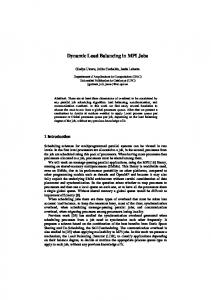
'c' values
'b' values
Normalized coefficients a, b, and were computed for every combination of decomposition, input data set, and processor count P in f2, 4, 8, 16, 32g, resulting in a table of triplets with 180 entries. An example where the decomposition is uniform geometric, the data set is polio, and the number of processors is 32 has the entry (a; b; ) = (3:59; 0:0032; 3:42 � 10 7 ). The performance improves by changing the decomposition to ORB leading to the values (a; b; ) = (1:64; 0:005; 3:42 � 10 7 ) (note the reduced a-value, representing load-balance improvement). These values are typical (as can be seen in figure 3 which shows all the data), in that the values for a are in the range 1.0 to 10, the values of b are typically less than 1=100 the value of a, and the values of are typically less than 1=105 of a. A general conclusion is that for modern parallel computers with values of g in 1 – 100 and L in 25 – 10000, the parallel overhead plus loadimbalance (amount that a > 1) far outweighs the cost of communication and synchronization on virtually all of the results in the study. Any decomposition that seeks a more evenly balanced load Comparison of Normalized Values will im(reduction of a) BSP prove performance far more 1 Fig. 3. A comparison showing the magnitude of difference than solutions that seek rebetween a and b, and a and for all (a; b; ) triplets in our duced communication (lower experiment. The values 0.1 of a are plotted along the x-axis. The b) or reduced synchronization b values are plotted with solid markers against a. Similarly, (lower ). Thus, even paralthe values are plotted 0.01along the y -axis with hollow markers lel computers with the slowagainst a. est communications hardware will execute well-balanced, spatially-decomposed MD simulations with good effi0.001 ciency. The graph0.0001 in figure 4 shows the effect of communication speed on the overall performance of the different decompositions. In this dataset, P is set to 32, and two different machine classes are-5examined. The first is a uniform memory access machine (UMA), 10 with (g; L) = (1; 128), representing machines such as the Cray vector processors that can supply values to processors at processor speed once an initial latency has been 10-6 is a non-uniform memory access machine (NUMA), much like charged. The second the SGI parallel computers and the Convex SPP. -7 There are two10interesting conclusions to be drawn from figure 4. The first is that executing MD on a machine with extremely high communication bandwidth (UMA) performs, in normalized terms, almost identically with machines with moderate com10-8 munications bandwidth. This is seen in the small difference between the same data 1 10 'a' values using the same decomposition, where the normalized execution cost for both architec-
a/b 2p a/c 2p a/b 4p a/c 4p a/b 8p a/c 8p a/b 16p a/c 16p a/b 32p a/c 32p
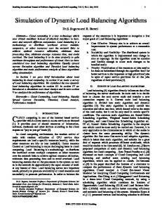
tures is nearly the same. The second interesting point in figure 4 is that decomposition matters much more than communications bandwidth. The decompositions that attempt to balance work and locality (ORB and spatial pairlist) have a bigger impact on performance than parallel computers with extremely high performance communications. This is a good indication that either the ORB or spatial pairlist decomposition should be used for a parallel implementation on any parallel computing hardware. The most significant conclusion drawn from this study is that load-balancing is by far the most important aspect of parallelizing non-bonded MD computations. This can be seen in the significantly larger values of a when compared to values of b and , as well as the results in figure 4 that show the improvement gained in using load-balanced decompositions. The spatial decomposition using pairlistlength as a measure shows the advantage that is achieved by increasing locality over the Fig. 4. This graph shows the normalized execution cost on
Effect of Communication Speed on Processors
Normalized BSP Execution Cost UMA: (g, L) = (1, 128) NUMA: (g, L) = (8,25)
non-spatial pairlist decompo- 32 processors, comparing different decomposition strategies Normalized BSP Execution Cost on 32 sition. These results are im- on machines with differing communication performance. portant not only in our work For the UMA architecture, (g; L) = (1; 128); for NUMA, 7 implementing simulators, but (g; L) = (8; 25). Note that the normalized cost of a proto others as well, guiding gram on a machine with very high performance communithem in the choices of their cation is only marginally better than machines with substan6 tially lower communication performance (except for pairlist parallel algorithms. decomposition).
5
4 Implementation of Dynamic Load Balancing in Molecular Dynamics 4
The results of the previous section are a stepping stone in the pursuit of our overall goal. In this section, we describe the parallelization using spatial decomposition for shared3 memory computers of our Sigma MD simulator. The performance results in this section show that the modeling provides a good starting point, but good scaling is difficult to 2 load-balancing. achieve without dynamic Optimizations in programs often hamper parallelization, as they usually reduce work in a non-uniform manner. There are (at least) two optimizations that hamper the 1 success of an ORB decomposition in Sigma. The first is the optimized treatment of water. Any decomposition based on atom count will have less work assigned when the percentage of atoms from water molecules is higher. 0
Uniform
Pairlist
ORB
Decomposition
Spatial Pairlist
SS-Cori SS-Cori Eglin (U Eglin (N Polio (U Polio (N
The second is the creation of atom groups, where between 1 and 4 related atoms are treated as a group for non-bonded interactions, so the amount of work per group can vary by a factor of 4. This optimization has the benefit of reducing the pairlist by a factor of 9, since the average population of a group is about 3. 4.1 A Dynamic Domain Decomposition Strategy One troubling characteristic of our average static parallel implementation was the work consistency of the imbalance in the per atom load over a long period. Typically, one processor had a heavier load than the Atom boundaries others, and it was this processor’s arbo b1 b2 b3 b4 Previous rival at the synchronization point that determined the overall parallel perforFuture bo b1 b2 b3 b4 mance, convincing us that an adaptive decomposition was necessary. To achieve an evenly balanced decomposition in our MD simulations, Fig. 5. Unbalanced work loads on a set of proceswe use past performance as a predic- sors. If the boundaries are moved as shown, then tion of future work requirements. One the work will be more in balance. reason this is viable is that the system of molecules, while undergoing some motion, is not moving all that much. The combination of this aspect of MD with the accurate performance information leads to a dynamic spatial decomposition that provides improved performance and is quick to compute. To perform dynamic load balancing, we rely on built-in hardware registers that record detailed performance quantities about a program. The data in these registers provide a cost-free measure of the work performed by a program on a processor-byprocessor basis, and as such, are useful in determining an equitable load balance. Some definitions are needed to describe our work-based decomposition strategy. – The dynamics work, wi , performed by each processor since the last load-balancing operation (does not include communication and synchronization costs) – The total work, W = P i=1 wi , since the last load-balancing operation – The estimated ideal (average) work, w = W=P , to be performed by each processor for future steps – The average amount of work, ai = wi =ni , performed on behalf of each atom group on processor i (with ni atom groups on processor i) – The number of decompositions, dx ; dy ; dz , in the x; y and z dimensions
P
4.2 Spatial Adaptation We place the boundaries one dimension at a time (as is done in the ORB decomposition) with a straightforward O(P ) algorithm. Figure 5 shows a single dimension split into n subdivisions, with n 1 movable boundaries (b0 and bn are naturally at the beginning and end of the space being divided). In Sigma, we first divide the space along
Number of Atom Groups on Each Processor
the x-dimension into dx balanced parts, then each of those into dy parts, and finally, each of the “shafts” into dz parts, using the following description. Consider the repartitioning in a single dimension as shown in figure 5. Along the x-axis, the region boundaries separate atoms based on their position (atoms are sorted by x-position). The height of a partition represents the average work per atom in a partition, which as stated earlier, is not constant due to density changes in the data and optimizations that have been introduced. Thus, the area of the box for each partition is wi , and the sum of the areas is W . The goal is to place Fig. 6. This graph shows two views of the adaptive decomposition working over time using 8 processors. The upper bi far enough from bi 1 such that the work (represented by traces show the number of T4-Lysozyme atom groups asto each processor. The lower traces show the percentarea) is as close to w as pos- signed Adaptive Spatial Decomposition age of time spent waiting in barriers by each process since sible. This placement of the over Time boundaries can be computed the previous balancing step. At step 0, an equal number of bound- atom groups is assigned to each processor, since nothing is in O(n) time for n800 aries. While this does not lead known about the computational costs. From then on, the deto an exact solution, a few it- composition is adjusted based on the work performed. erations of work followed by balancing yield very good solutions where the boundaries settle down. 700 Figure 6 shows the boundary motion in Sigma as the simulation progresses. Initially, space is decomposed as if each atom group causes the same amount of work. This decomposes space using ORB such that all processors have the same number of atom groups. As the simulation progresses, boundaries are moved to equalize the load based 600 on historical work information. This makes the more heavily loaded spaces smaller, adding more volume (and therefore atoms) to the lightly loaded spaces. As the simulation progresses, the number of atom groups shifted to/from a processor is reduced, but still changing due to the dynamic nature of the simulation and inexact balance.
40%
30%
20%
4.3 Results
10%
Rebalancing Step
0% 8
9
Percentage of time spent waiting
500
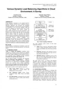
We have tested the implementation on several different parallel machines, including SGI Origin2000, SGI400 Power Challenge and KSR-1 computers. Figure 7 shows the performance of several different molecular systems being simulated on varying numbers of processors. The y -axis shows the number of simulation steps executed per second, which is indeed the metric0of most1concern2 to the scientists We7 ran 3 4 using the 5 simulator. 6
p p p p p p p p
tests using decompositions where we set P = (dx � dy � dz ) to 1, 2, 4, 6, 8, 9, 12, and 16. There are several conclusions to be drawn from the performance graph, the most important of which is the scaling of performance with increasing processors. The similar slopes of the performance trajectories for the different datasets shows that the performance scales similarly for each dataset. The average speedup on 8 processors for the data shown is 7.59. The second point is that the performance difference between the two architectures is generally very small, despite the improved memory bandwidth of the Origin 2000 over the Power Challenge. Our conjecture to explain this, based on this experiment and the BSP modeling in the previous section, is that the calculation of non-bonded interactions involves a small enough dataset such that most, if not all, atom data can remain in cache once it has been fetched.
5 Conclusions
Simulation Steps per Second
We are excited to achieve Parallel Performance of Sigma performance that enables in100 SS-Corin Perfect Speedup teractive molecular dynamT4 Perfect Speedup SS-Corin (Origin2000) ics on systems of molecules SS-Corin (Challenge) relevant to biochemists. Our T4-Lysozyme (Origin2000) performance results also enT4-Lysozyme (Challenge) able rapid execution of large 10 timescale simulations, allowing many experiments to be run in a timely manner. The methodology de1 scribed shows the use of high1 10 level modeling to understand Processors what the critical impediments to high-performance are, followed by detailed implemen- Fig. 7. Parallel Performance of Sigma. This graph shows the tations where optimizations number of simulations steps per second achieved with sev(including model violations) eral molecular systems, T4-Lysozyme (13642 atoms), and can take place to achieve even SS-Corin (3948 atoms). The data plotted represent the performance of the last 200fs (100 steps) of a 600fs simulation, better performance. Prior to our BSP model- which allowed the dynamic decomposition to stabilize prior ing study, we could only con- to measurement. A typical simulation would carry on from 6 jecture that load-balancing this point, running for a total of 10 fs (500,000 simulation was the most important as- steps) in simulated time, at roughly these performance levpect of parallelism to explore els. for high performance parallel MD using a spatial decomposition. Our BSP modeling supports this claim, and also leads us to the conclusion that the use of 2 or 4 workstations using ethernet communications should provide good performance improvements, despite the relatively slow communications medium. Unfortunately, we have not yet
demonstrated this, as our implementation is based upon a shared-memory model, and will require further effort to accommodate this model. Our BSP study also shows that, for MD, processor speed is far more important than communication speed, so that paying for a high-speed communications system is not necessary for high performance MD simulations. This provides economic information for the acquisition of parallel hardware, since systems with faster communication usually cost substantially more. And finally, we’ve shown that good parallelization strategies that rely on information from the underlying hardware or operating system can be economically obtained and effectively used to create scalable parallel performance. Much to our disappointment, we have not been able to test our method on machines with large numbers of processors, as the trend with shared-memory parallel computers is to use small numbers of very fast processors. We gratefully acknowledge the support of NCSA with their “friendly user account” program in support of this work.
References 1. R. H. Bisseling and W. F. McColl. Scientific computing on bulk synchronous parallel architectures. Technical report, Department of Mathematics, Utrecht University, April 27 1994. 2. John A. Board, Jr., Ziyad S. Hakura, William D. Elliott, and William T. Rankin. Scalable variants of multipole-accelerated algorithms for molecular dynamics applications. Technical Report TR94-006, Electrical Engineering, Duke University, 1994. 3. David A. Case, Jerry P. Greenberg, Wayne Pfeiffer, and Jack Rogers. AMBER – molecular dynamics. Technical report, Scripps Research Institute, see [9] for additional information, 1995. 4. Terry W. Clark, Reinhard v. Hanxleden, J. Andrew McCammon, and L. Ridgway Scott. Parallelizing molecular dynamics using spatial decomposition. In Proceedings of the Scalable High Performance Computing Conference, Knoxville, TN, May 1994. Also available from ftp://softlib.rice.edu/pub/CRPC-TRs/reports/CRPC-TR93356-S. 5. Tom Darden, Darrin York, and Lee Pedersen. Particle mesh ewald: An n log(n) method for ewald sums in large systems. J. Chem. Phys., 98(12):10089–10092, June 1993. 6. Yuan-Shin Hwang, Raja Das, Joel H. Saltz, Milan Hodoˇscˇ ek, and Bernard Brooks. Parallelizing molecular dynamics programs for distributed memory machines: An application of the chaos runtime support library. In Proceedings of the Meeting of the American Chemical Society, August 21–22 1994. 7. Jonathan Leech, Jan F. Prins, and Jan Hermans. SMD: Visual steering of molecular dynamics for protein design. IEEE Compuational Science & Engineering, 3(4):38–45, Winter 1996. 8. Mark Nelson, William Humphrey, Attila Gursoy, Andrew Dalke, Laxmikant Kale, Robert D. Skeel, and Klaus Schulten. NAMD - a parallel, object-oriented molecular dynamics program. Journal of Supercomputing Applications and High Performance Computing, In press. 9. D.A. Pearlman, D.A. Case, J.W. Caldwell, W.R. Ross, T.E. Cheatham III, S. DeBolt, D. Ferguson, G. Seibel, and P. Kollman. AMBER, a computer program for applying molecular mechanics, normal mode analysis, molecular dynamics and free energy calculations to elucidate the structures and energies of molecules. Computer Physics Communications, 91:1–41, 1995. 10. L. F. Valiant. A bridging model for parallel computation. CACM, 33:103–111, 1990.