Dynamic Modification of System Structures Using LLPNs final draft Berndt Farwer1 and Kundan Misra2 1
2
University of Hamburg, Department of Computer Science,
[email protected] Department of Computer Science, University of Warwick,
[email protected]
Abstract. In this paper we aim to set up a framework for object Petri net semantics, allowing the modification of object net structures at runtime. The approach uses linear logic Petri nets (LLPNs) and performs the structure modification on a linear logic encoding of the object net. In addition, Valk’s self-modifying Petri nets are shown to be subsumed by LLPNs. We expand on the existing theory of Farwer’s LLPNs, which are Petri nets with linear logic formulae as tokens. This work in progress uses intuitionistic linear logic as the basis of a method for ensuring desirable properties—such as termination or non-termination—of P/T nets, coloured Petri nets and LLPNs.
1
Background and Motivation
Petri nets are well-known models for concurrent and reactive systems. A placetransition net (P/T net) is a type of Petri net with places which can contain tokens and transitions that are connected by directed, weighted arcs. Diagramatically, places are represented by circles and transitions by rectangles. The precondition of a transition is the number of tokens needed in each place for the transition to be enabled, and is indicated by the weights of the incoming arcs. The postcondition of a transition is the number of tokens generated in each place by the firing of the transition, and is indicated by the weights of the outgoing arcs. A transition fires when its precondition is satisfied, after which its postcondition is generated. This is shown in Figure 1. P/T nets have been extended in several ways. Coloured Petri nets (CPNs) were introduced under the name of “high-level Petri nets” by Jensen [16]. CPNs
place1
transition 2
3
place2
transition fires
place1
transition 2
Fig. 1. Transition firing in a P/T net
3
place2
place1
transition 2
3
place1
place2
transition 2
3
place2
(a) Transition firing in an object Petri net
p21 ⊗!(p21 !p32 )
p21 ⊗!(p21 !p32 )
(b) Corresponding transition firing in an LLPN Fig. 2. Object Petri net vs. linear logic Petri net
allow tokens to have different values. Each place is associated with a set of allowable values (“colours”) and that set corresponds to a data type (“colour set”). The tokens inside a place must be taken from the colour set associated with the place. Any transition in a CPN may have a “guard function”, which allows the designer to specify complex criteria on the incoming arcs. An equivalent CPN without a guard can always be constructed by unfolding the CPN. Some work has been done to express CPNs using linear logic [8]. Also, Lilius explains how CPNs can be described using linear logic by first converting a CPN to a corresponding P/T net [18] by creating a place for each value/colour. This quickly becomes unworkable for any practical use, because the colour set (i.e. data type) of any place is often infinite (e.g.. N). Object Petri nets allow various structured objects as tokens, including P/T nets themselves. When P/T nets are used as tokens of a CPN, the token P/T nets are called object nets and the CPN whose places contain token nets is called the system net. A simple example of an autonomous system net transition firing is shown in Figure 2. Here the object net is simply moved to a different place of the system net. Other more complex moves involving synchronisation of system and object net transitions are possible, but cannot be discussed here. Farwer devised a type of CPN in which the tokens are formulae from linear logic formulae called linear logic Petri nets (LLPNs) [9]. LLPNs are distinct from CPNs because they allow tokens (linear logic formulae) to interact in the places under the proof rules of linear logic. Suppose the linear logic formulae J!K and J enter a place b. Then J and J!K are consumed to produce K. Now K alone is available to the output transitions of b. The firing rule of LLPNs is that a transition will fire if for each input place of the transition, the proof tree of the
formulae in the place has a step with the transition’s precondition [8]. LLPNs are convenient for modelling real-world systems and make the large body of linear logic theory available for modelling and analysing complex systems. Linear logic has been used as a medium through which to talk about sequential and concurrent programming-language semantics [1], and has been facilitated for giving semantics for P/T nets [3, 7, 9, 23]. Usually, these treatments are restricted to intuitionistic linear logic (ILL). Thus, we restrict the formulae tokens of LLPNs to ILL formulae. Brown, Gurr and de Paiva developed an ILL proof theory for P/T nets [4]. They also gave a category theoretic proof that linear logic is a specification language for P/T nets. These last two results have been extended to LLPNs [21]. Meseguer and others used functorial embeddings of the category of P/T nets into categories related to linear logic to explain the connection between P/T nets and linear logic [19, 20]. A categorical semantics of the simulation (i.e. refinement and abstraction) of P/T nets has also been developed [4] and this has been extended to LLPNs [21]. Treatments by Engberg, Winskel and Farwer do not rely so much on category theory [7–9]. As put by Sangiorgi and Walker [22], “Mobile systems, whose components communicate and change their structure, now pervade the informational world and the wider world of which it is a part.” Heeding this observation requires that dynamic modification of Petri net structures be included in any serious object Petri net formalism. In this paper we give some ideas of how this can be achieved and study a possible application. It is often necessary to ensure that a system has some desirable property, such as that it must or must not terminate. We will show how the use of linear logic, first order linear logic and second order linear logic can greatly simplify the augmenting of P/T nets, CPNs and LLPNs to ensure desirable properties. This is a seminal stage in developing a framework for systems that are modelled by Petri nets to ensure their own desirable behaviour without external intervention. This might lead towards a standard environment into which we can “plug” a Petri net to ensure that it has desirable properties.
2
Translation between LLPNs and Object Petri Nets
A revision of the rules of intuitionistic linear logic and the definition of object Petri nets are given in the appendices. Note, that the definition of a linear logic Petri net in the following section differs slightly from the definition given in [11], in that it generalises the arc inscriptions to multisets of linear logic formulae, rather than multisets of variables only. Also, a capacity is introduced for the places of an LLPN. Finally, the firing rule is generalised to incorporate autonomous derivation of the token formulae. A variety of different high-level Petri nets are actively used for systems engineering (cf. [30]), all of which extend the basic formalism of place/transition nets or P/T nets. The definition of P/T nets is now recalled for reference.
Definition 1 (P/T net). A P/T net is a tuple (P, T, F, W ) with disjoint sets of places P and transitions T ; the function F ⊆ (P × T ) ∪ (T × P ) defines the flow relation; and the function W : (P × T ) ∪ (T × P ) → N with W (x, y) = 0 if and only if (x, y) ̸∈ F defines the arc weights. A marked P/T net or P/T net system is a tuple (P, T, F, W, m0 ) where (P, T, F, W ) is a P/T net and m0 : P → N is the initial marking. An arc with weight zero has the same practical effect as an arc that does not exist, and so we regard these notions as equivalent. In the following, a P/T net is called an ordinary Petri net if ∀(x, y) ∈ F.W (x, y) = 1 is true for that P/T net. 2.1
Linear Logic Petri Nets
We denote by LA the set of all ILL formulae over the alphabet A and by SLA the set of sequents over LA . The shorthand B A , where A and B are sets, to denotes the set of all functions A → B. We take 0 ∈ N. Definition 2 (Linear Logic Petri net, LLPN). A linear logic Petri net is a 6-tuple (P, T, F, Λ, G, v, m0 ), where: – – – – –
P is the set of places T is the set of transitions, such that P ∩ T = ∅ F ⊆ (P × T ) ∪ (T × P ) is the flow relation Λ maps each element of P ∪ T to a fragment of (propositional) linear logic v is a function defined on (P × T ) ∪ (T × P ) which maps pairs (x, y) to multisets of variables drawn from the set of variables V in LΛ(p) where p ∈ {x, y}. Denote by Vt the set of variables on arcs adjacent to t, i.e. Vt = {v ∈ V | ∃p ∈ • t ∪ t • .v ∈ v(p, t) ∪ v(t, p)} s – the guard function G : T → 2LΛ(t) maps each transition to a set of sequents over LΛ(t) – the initial marking is some function m0 with p +→ np for every p ∈ P where np ∈ NLΛ(p) .
For a formula l ∈ LA we denote by ml (p) the number of occurrences of the formula l in the place p for the marking m. The marking of a place!is extended to a set of places M ⊆ P by the multiset union, i.e. m(M ) := p∈M m(p). The weight function v assigns to each arc a multiset of variables. If there is no arc between nodes x and y the weight function denotes the empty multiset. In symbols, if (x, y) ̸∈ F then w(x, y) is the empty multiset. We denote the precondition of a transition t by • t := {p ∈ P | (p, t) ∈ F } and the postcondition of t by t • := {p ∈ P | (t, p) ∈ F }. Definition 3 (marking’s proof trees). Given a marking m and place p, the proof trees of m(p) are all possible proof trees that can be formed with at most the formulae from the multiset m(p) together with some axioms and tautologies of the calculus as their premises, i.e. leaves of the proof trees. We denote this set of proof trees by Φ(m(p)). The " set of proof trees of a marking m is denoted Φ(m) and is given by Φ(m) := p∈P Φ(m(p)).
Definition 4 (independent formulae). The set of multisets of formulae that can hold independently in a proof tree Φ is denoted I(Φ). This means that for every multiset of formulae ΦF ∈ I(Φ), all formulae in ΦF can hold independently in the proof tree Φ. For example, suppose Φ is the proof tree [24]: C, Γ, A
C, Γ, B
C, Γ, A&B
D, Γ ′
C ⊗ D, Γ, Γ ′ , A&B $ # $ ′ ′ For ΦF1#= {C, Γ, A}, {C, Γ, B}, {D, Γ } , Φ {C, Γ, A&B}, {D, Γ } F 2 = $ and ΦF3 = {C ⊗ D, Γ, Γ ′ , A&B} , we get I(Φ) = ΦF1 ∪ ΦF2 ∪ ΦF3 . #
Definition 5 (binding). A binding for a Linear Logic Petri net transition t is a mapping β : vt → LΛ , such that % % LΛ(p) β(x) ∈ p∈ • t∪t • x∈Vt
and all sequents σ ∈ G(t)(β) are derivable in Λ(t). As we are only discussing propositional calculi there is no need for unification at this point. Definition 6 (enablement). A transition t ∈ T is enabled with binding β if and only if there exists a t-binding satisfying G(t), such that there is one occurrence of β(X) in the place p ∈ • t for each occurrence of X in W (p, t), i.e. ∀p ∈ • t.∀X ∈ W (p, t).m(p)(β(X)) ≥ W (p, t)(X) The satisfaction of a guard formula is defined as its derivability in the Linear Logic sequent calculus. Definition 7 (successor marking). Transition t may occur taking the marking m to reach the successor marking m′ according to the following rule for every place p in P and every variable X that appears in the arc inscription of any arc connected to t: m′ (p)(β(X)) = m(p)(β(X)) − W (p, t)(β(X)) + W (t, p)(β(X)) Autonomous derivations among formulae residing in the same place are possible iff there exists a proof tree with the derived formula as consequence. Since the firing rule depends also on proof trees, a large number of markings are equivalent. For example, the marking m(p) = {A} will enable a transition t if and only if the marking m′ (p) = {B!A, B} enables the transition t, as does the markings {(B!A) ⊗ B} This means that it is often convenient to think in terms of sets of equivalent markings with respect to the enablement of transitions. & ' () We can express the equivalence between m(p) and m′ (p) by I Φ m(s) = & ' () I Φ m′ (s) . Since equality is an equivalence relation, we immediately obtain equivalence classes of markings.
2.2
Interpreting object Petri nets as LLPNs
There is a strong correspondence between intuitionistic linear logic (ILL) formulae and P/T nets [6, 3, 7, 11, 12]. This means that the object nets of an object Petri net can be regarded as ILL formulae. In this way, we can regard an object Petri net as an LLPN. Conversely, an LLPN can be regarded as an object Petri net. We recall Farwer’s canonical ILL formula for a P/T net. Definition 8 (canonical formula for a P/T net). Let N = (P, T, F, W, m0 ) be a P/T net system. Then the canonical formula ΨILLP N (N ) for N is the tensor product of the following formulae: – For each transition t ∈ T with non-empty preconditions postconditions t • , &* ) * ! pW (p,t) ! q W (t,q) . p∈ • t
•
t and non-empty
q∈t •
– For the current marking m and each place p ∈ P with m(p) = n ≥ 1, we include pn . The special cases of where the precondition or postcondition of transition t is empty are accounted for in Definition 8. Explicitly, for each transition t where • t = ∅, we include the formula & ) &* ) * ! 1! q W (t,q) or equivalently ! q W (t,q) , q∈t •
q∈t •
and for each transition t where t • = ∅, we include the formula &* ) &' * (⊥ ) ! pW (p,t) ! ⊥ or equivalently ! pW (p,t) . p∈ • t
p∈ • t
It is now clear that, given an object Petri net, we can regard the object nets as ILL formulae using Definition 8. Thus, we can regard any object Petri net, as defined in Appendix A as an LLPN. The above suggests a reverse translation, from ILL to P/T nets. In order to interpret ILL formulae without the modality ! as P/T nets, we require extended P/T nets which include the concept of disposable transitions [10]. However, we will not require the reverse translation in this work. Aside from the reverse of the translation suggested by Definition 8, work by other authors provide a P/T net interpretation of full ILL [6, 7].
3
Why study dynamic structures?
At a first glance the notion of “dynamic structure” may seem to be an oxymoron. Taking a closer look at the direction of information technology and its
applications, it is clear that the connectedness of remote systems has become the major factor in many areas of computation and communication. The main example is of course the Internet. The Internet and even metropolitan and wide area networks (MANs and WANs) are reconfigured frequently, and so there is dynamism in the overall structure of these networks. This is accommodated, for instance, by the development of dynamic databases, where the topology is subject to permanent changes which must be taken into account by each new request. There are different kinds of dynamism, two of which will be discussed in this paper: (i) dynamic reconfiguration of resource-related quantitative aspects of systems, and (ii) dynamic change of data flow, i.e. modification of the physical layout of a system. The former is a kind of modification tackled by the self-modifying nets defined by Valk [25]. The latter has not yet been convincingly integrated into a Petri net-based modelling formalism. We show that both modification approaches are subsumed by LLPNs in Section 4 and in Section 5.
4
Self-modification and LLPNs
In this section some aspects of self-modification for Petri nets are discussed. In particular, it is shown that the self-modifying nets of Valk [25] can be simulated by LLPNs. A self-modifying Petri net is essentially a P/T net that can have linear expressions, with variables drawn from the place names of the net, as arc weights. That is, the weight of an arc from place p to transition t is given by an expression + + aq q where aq ∈ N for all q ∈ P , with the meaning W (p, t) = aq m(q). q∈P
q∈P
If the arc expression for an arc (p, t) ∈ F of a self-modifying net includes a coefficient for p greater than one, then the net is not well-formed since transition t cannot be enabled. The self-modifying nets discussed below will be assumed to be well-formed. An example of a self-modifying net transition is given in Figure 3(a). This transition can be simulated by the LLPN transition shown in Figure 3(b). Construction 9 gives a general transformation of self-modifying nets into LLPNs. Construction 9. Let N be a well-formed self-modifying Petri net with set of places P , set of transitions T , flow relation F , and initial marking m0 . Construct an LLPN N ′ := (P, T, F ′ , Λ, G, v, m0 ′ ) such that F ′ := F ∪ F −1 ∪ {(p, t) ∈ P × T | ∃p′ ∈ P.p has non-zero coefficient in W (p′ , t)} ∪ {(t, p) ∈ T × P | ∃p′ ∈ P.p has non-zero coefficient in W (t, p′ )}
Yœ Xœ
Yπ
p
t
t Xp ⊢ Xr ⊗ Yp
X® r
q
Xπ
p
X√
Xv ⊗ Xv ⊗ Yq ⊢ Xq
r
2v
v
q
(a) Transition of a self-modifying net referring to places r and v
(b) LLPN transition simulation t from subfigure (a)
Fig. 3. A transition of a self-modifying net with arc weights referring to the markings of places r and v simulated by an LLPN transition
Λ is the set of all finite tensor products built with the single propositional variable a. The initial marking is given as follows: ∀p ∈ P.m0 ′ (p) := am0 (p) The arc inscriptions and guards of N ′ are defined according to the following rules: 3 1. If (p, t) ∈ F has an arc expression α(p,t) that does not contain p, then the LLPN will have an arc from each place q ∈ P occurring in α to t with inscription Xq . A reversed arc (t, p) with inscription Yp is introduced. The guard for transition t then includes the sequent Xp ⊢ Yp ⊗
*
Xq .
q∈α(p,t)
This tensor product depends on the multiset α(p,t) and so it takes into account the coefficients in the arc inscription of N . 2. If the arc expression of (p, t) ∈ F contains p (with coefficient one) then the arc acts as a reset arc and is represented by (p, t) ∈ F ′ with inscription Xp and with guard G(t) = {Xp ⊢ Xp }. The reverse arc (t, p) has no inscription and so can be omitted. If other place names appear in the arc expression of (p, t) ∈ F , then they are treated as in case 1. 3. If (t, p) ∈ F has an arc expression α(p,t) , then the LLPN will have an arc from each place q ∈ P occurring in α to t with inscription Xq . A reversed arc (t, p) with inscription Yp is newly introduced. 3
Arc inscriptions of self-modifying nets can be viewed as multisets of place names. In the sequel, multisets are sometimes written as formal sums for convenience.
In addition to the sequents introduced to the guard in 1 and 2, the guard for transition t contains the sequent * Yp ⊗ Xq ⊢ Xp q∈α(t,p)
where the tensor product depends on the multiset α(t,p) . The flow relation F ′ in Construction 9 unfolds the arcs of the self-modifying net so that each arc depends on the marking of only one place. Note also that in any reachable marking of the LLPN from Construction 9, the entire marking of each place is treated as (at most) one formula. Theorem 1. The LLPN labelled N ′ in Construction 9 simulates the self-modifying net N with respect to the following simulation relation on markings, mapping multiplicities of tokens to tensor products: , .|P | |P | n ∼⊆ N × a where (n1 , . . . , n|P | ) ∼ (an1 , . . . , an|P | ). n∈N
In Theorem 1, N and N ′ have the same set of possible firing sequences and the same reachability set with respect to the ∼ relation.
Proof. Immediate from the construction, since no autonomous derivations are possible for the restricted class of formulae allowed as tokens. Intuitively, the marking of each p ∈ P given by m(p) = n in N is simulated by m(p) = a/ ⊗ .01 . . ⊗ a2 = an in N ′ . n
Using ideas from Farwer and Lomazova [13], a self-modifying net transition can be encoded by a first-order intuitionistic linear logic formula containing a binary locality predicate P to specify that some formula φ resides in place p by P (p, φ). For example, the transition from Figure 3(a) would be represented as the universally quantified formula !(p(Xr ⊗ Yp )⊗ q(Yq )⊗ r(Xr )⊗ v(Xv ) ! p(Yp )⊗ q(Xv ⊗ Xv ⊗ Yq )⊗ r(Xr )⊗ v(Xv )) where p(X) is short for P (p, X). A similar encoding is possible, when enriching ILL with a modality for locality, such as the modal linear logic for distribution and mobility (DMLL) [2]. The simulation in Theorem 1 does not faithfully retain concurrency. To remedy this, we would have to equip LLPNs with the concept of test arcs, which are used in other areas of Petri net theory. Nevertheless, our result shows that in interleaving semantics, self-modifying nets can concisely be simulated by LLPNs. Self-modifying nets have already been generalized to G-nets [5]. G-nets are a type of self-modifying net which allow polynomials of degree greater than one, where the variables of the polynomials are the place names of the net. There is no obvious way of extending Construction 9 to G-nets. Indeed, it is not possible to express polynomials of degree greater than one in propositional ILL if we use the ILL-representation of linear polynomials given in Construction 9. Further discussion of G-nets is beyond the scope of this paper due to space limitations.
5
Structural modification
5.1
Motivating object net modification
Many common P/T net properties have an evident extension to LLPNs. Some examples follow. Definition 10 (termination). An LLPN is terminating if there is no infinite firing sequence. Definition 11 (deadlock-freedom). An LLPN is deadlock-free if each reachable marking enables a transition. Definition 12 (liveness). An LLPN is live if each reachable marking enables a firing sequence containing all transitions. These properties point the way to a large class of situations in which it is necessary to be able to represent modification of object nets by the system net. For example, it is often necessary to ensure that some software process terminates. On the other hand, it might be necessary to ensure that a communication or control process never terminates. There are standard ways of detecting termination without using LLPN features which addresses the first of these. Below, the possibility of unwanted nontermination in the form of infinite loops will be addressed. Our approach will involve the modification of a transition in the object net (or, to be more precise, the linear logic encoding of the transition). In order to be able to ensure that exactly and only the desired modification is carried out, we first introduce the s-canonical formula of a P/T net. This modification of the standard canonical formula defined by Farwer [10] adds a fresh propositional symbol to the premise of each linear implication representing a transition. The reason for introducing this additional premise is to force the transition to synchronise with a system net transition, whereby we will be able to take some action after any object net transition fires.4 Definition 13 (s-canonical formula). Let N = (P, T, F, W, m0 ) be a P/T net. Then the s-canonical formula for N is the tensor product of: – For each transition t ∈ T with non-empty preconditions • t and non-empty postconditions t • ) &* * ! pW (p,t) ⊗ δ ! q W (t,q) ⊗ δ , p∈ • t
q∈t •
where δ and δ are fresh propositional variables, and – pm(p) for the current marking m and each place p ∈ P with m(p) ≥ 1. 4
This restricts concurrency in the object net, which can granularly be regained by introducing additional modes for the respective system net transition(s). This is not discussed further here, in order not to distract the reader from the main idea and to keep the examples simple.
x
s-canonical formula of a P/T-net or CPN
t y
p
x⊗δ ⊢ y⊗δ •
name
s
Á
c
Á,Á
…
q
•
name
Á Á
a
Fig. 4. Petri net augmentation to detect a repeated net marking
5.2
Detecting and addressing infinite loops
A net with initial marking m0 is potentially non-terminating if (but not only if) the same marking appears twice in the firing sequence starting at initial marking m0 . That is, we have: m0 → m1 → · · · → mk → mk+1 → · · · → mn → mk → . . . . for some 0 ≤ k ≤ n. A method follows for augmenting a net to detect and address non-termination in this class of cases. Non-termination in a CPN N can be detected by a concise LLPN construction. A “camera” place connects to all other places via “snapshot” transitions. Every transition of N is augmented so that each occurrence of the net adds an “unsnapped marker” token to all places. The presence of unsnapped marker tokens causes a snapshot to be taken of the entire net. That is, a token that is an ILL formula representation of the current marking of N is stored in a camera place with LLPN functionality. An evident ILL formula denoted Ψ can be added to the camera place as a token which responds to the presence of two identical snapshots. The formula Ψ quantifies over values drawn from all colour sets of the CPN. When there are two identical snapshots in the camera place, a token is sent to a place to indicate non-termination. Figure 4 illustrates this. The token formula in place p represents the original net N under consideration, encoded here in s-canonical form. Transition t allows any derivation that corresponds to the firing of an enabled transition in the object net. Each occurrence of t places a black token in the place triggering transition s that places a snapshot of the encoded object net in the camera place c. By requiring the presence of two identical object net snapshots in c, transition a is only enabled if a marking in the object net has recurred. Transition a can then trigger an action not shown in this figure. For practical use, the two solid
A
B
Fig. 5. Object net corresponding to A⊗!(B!A)⊗!(A!B)
transitions have to be “immediate transitions”, meaning that they have to fire immediately when they are enabled. Thus, the type of potential non-termination described above can be detected in an LLPN. But how is a loop to be addressed when it arises? We consider a specific case. Consider a formula of the form A⊗!(B!A)⊗!(A!B) where A and B are atomic, appearing in mk mk+1 . . . mn the part of the firing sequence that repeats. Note that this linear logic formula corresponds to the object net in Figure 5. Suppose that many transitions require something representing an energy token denoted E. An obvious way of checking the progress of the repeating firing sequence is to substitute for any token of the form !(A!B) the token !(A ⊗ E!B) using: 3 4 3 4 !(B!A)⊗!(A!B) ! !(B!A) ⊗ !(A ⊗ E!B) .
(1)
A net to which the above can be applied might typically have a place containing some finite supply of energy, represented by a finite number of E tokens. In order that a token of the form !(A!B) be recognizable and the formula (1) sent to the appropriate places, variables are needed for atomic symbols. In particular, the following formula could be used in the guard of the transition t of the LLPN: !(x!y) ! !(x ⊗ E!y), which allows the derivation of: 35 4 3 4 6 !(x!y) ! !(x ⊗ E!y) ⊗ !(y!x)⊗!(x!y) ⊢ !(y!x) ⊗ !(x ⊗ E!y) .
The energy requirement represented by E must be made specific to the applicable formula !(x!y) to ensure that these behaviour-modification linear logic formulae do not interfere with such formulae in other places. Therefore, the symbol Exy is used to index the E. Another possible way of dealing with this kind of modification is to provide additional formulae within the places that contain token formulae that are to be modified and rely on the autonomous derivations possible in LLPNs. This approach, while possible, would offer little control over the time at which modification occurs. This approach would also require quantification over atomic symbols for detecting the need for a modification and subsequent deployment of
appropriate subformulae to carry out the modification: ∀x, y ∈ A. 3 4 35 4 6 !(y!x) ⊗ !(x!y) ! !(x!y) ! !(x ⊗ Exy !y) ⊗ !(y!x) ⊗ !(x!y) (. 2)
Using the formula (2) will cause the infinitely cycling process to cease when the energy is exhausted or the energy requirement will be stepped up if the process repeats again. A problem remains in !(A!B) producing an indeterminate number of duplicates of A!B. At present, the only known way of addressing this problem is by partitioning the reduction (according to the rules of linear logic) of linear logic formulae using a method by Farwer which develops Girard’s multi-region logical calculus [14, 15, 12]. This method was originally motivated by the need to deal with disposable transitions, i.e. transitions that are allowed to occur only a finite number of times and which no longer exist as soon as this “capacity” is exceeded. It is possible to progress even further, beyond (2) to second-order ILL , by quantifying in the following way: ∀x, y ∈ LA and this would prevent nontermination in a much larger class of situations. 5.3
Alternative approach using transition guard
We now outline a different approach for the modification of the object net encoding. In this approach, the net modification is carried out by the guard of a single transition. The steps follow: – Define a partial order ≺ on the set of canonical formulae for a Petri net. The partial order can be defined on the length of a formula and is introduced to deal with the non-uniqueness of Petri net encodings due to the possible replication of the exponential subformulae representing the transitions. – A formula for a net is in reduced canonical form (RCF) if it is a lower bound of the canonical net representations with respect to ≺. In general, there is not a unique representation in RCF, since the tensor is commutative. Thus, there exist equivalent formulae of the same length. – Apply the modification on an s-canonical net representation in RCF utilising a guard of the LLPN. For example, let x and y be in RCF and let x1 and x2 comprise tensor products of atoms, representing markings of the object net. Then the following guard of a system net transition can be used to modify the object net encoding according to the ideas in Section 5.2: # x ⊢ Γ ⊗ !(x1 ⊗ A!x2 ), Γ ⊗ !(x1 ⊗ A!x2 ) ⊗ (!(x1 ⊗ A!x2 ) ! !(x1 ⊗ A ⊗ E!x2 )) ⊢ Γ ⊗ !(x1 ⊗ A ⊗ E!x2 ), $ Γ ⊗ !(x1 ⊗ A ⊗ E!x2 ) ⊢ y .
By restricting the formulae to the reduced canonical formulae of nets, we avoid the replication anomalies discussed in previous papers.
6
Conclusions and future work
We have shown a straightforward way to simulate self-modifying Petri nets by linear logic Petri nets. Furthermore, we have given a framework for using LLPNs to modify at run-time a token formula representing an object net. This continues our investigation into appropriate semantics for object Petri net formalisms by giving, for the first time, the possibility of dynamic structural modifications. This extends the benefits of object-based modelling with the flexibility needed for modelling highly dynamic distributed systems that have gained an immense importance in recent years. From a practical point of view, we are seeking to leverage the theory of ILL to do essentially what a compiler does with a computer program. That is, a software program is made to sit in a certain infrastructure which ensures that the program executes in a way that has certain desirable properties. However, the tokens that are used to produce a desired, or more desirable, behaviour may not be so obvious as in the case given in this paper. A general framework is required to systematically determine by using first or second-order ILL the most appropriate ILL formula tokens to use. Linear logic allows far reaching modifications to be modelled. It is an open problem, how these possibilities should be restricted in order to retain desirable properties and preserve traditional results on Petri nets.
References 1. S. Abramsky. Computational interpretations of linear logic. Theoretical Computer Science, 111:3–57, 1993. 2. N. Biri and D. Galmiche. A modal linear logic for distribution and mobility. Talk given at LL’02 of FLoC’02, 2002. 3. C. Brown. Linear Logic and Petri Nets: Categories, Algebra and Proof. PhD thesis, AI Laboratory, Department of Computer Science, University of Edinburgh, 1991. 4. C. Brown, D. Gurr, and V. de Paiva. A linear specification language for Petri nets. Technical Report 363, Computer Science Department, Aarhus University, 1991. 5. C. Dufourd, A. Finkel, and Ph. Schnoebelen. Reset nets between decidability and undecidability. In Proceedings of the 25th International Colloquium on Automata, Languages, and Programming (ICALP’98), volume 1443 of LNCS. Springer-Verlag, 1998. 6. U. Engberg and G. Winskel. Petri nets as Models of Linear Logic. In A. Arnold, editor, Proceedings of Colloquium on Trees in Algebra and Programming, volume 389 of Lecture Notes in Computer Science, pages 147–161, Copenhagen, Denmark, 1990. Springer-Verlag. 7. U. H. Engberg and G. Winskel. Linear logic on Petri nets. Technical Report ISSN 0909-0878, BRICS, Department of Computer Science, University of Aarhus, DK-8000 Aarhus C Denmark, February 1994.
8. B. Farwer. Towards linear logic Petri nets. Technical report, Faculty of Informatics, University of Hamburg, 1996. 9. B. Farwer. A Linear Logic View of Object Systems. In H.-D. Burkhard, L. Czaja, and P. Starke, editors, Informatik-Berichte, No. 110: Workshop Concurrency, Specification and Programming, pages 76–87, Berlin, September 1998. HumboldtUniversit¨ at. 10. B. Farwer. Linear Logic Based Calculi for Object Petri Nets. PhD thesis, Fachbereich Informatik, Universit¨ at Hamburg, 1999. Published by Logos Verlag, 2000. 11. B. Farwer. A Linear Logic View of Object Petri nets. Fundamenta Informaticae, 37:225–246, 1999. 12. B. Farwer. A multi-region linear logic based calculus for dynamic petri net structures. Fundamenta Informaticae, 43(1–4):61–79, 2000. 13. B. Farwer and I. Lomazova. A systematic approach towards object-based petri net formalisms. In D. Bjorner and A. Zamulin, editors, Perspectives of System Informatics, Proceedings of the 4th International Andrei Ershov Memorial Conference, PSI 2001, Akademgorodok, Novosibirsk, pages 255–267. LNCS 2244. Springer-Verlag, 2001. 14. J.-Y. Girard. Linear logic: its syntax and semantics. In Girard et al. [15], pages 1–42. 15. J.-Y. Girard, Y. Lafont, and L. Regnier, editors. Advances in Linear Logic. Number 222 in Lecture notes series of the London Mathematical Society. Cambridge University Press, 1995. 16. K. Jensen. An Introduction to High-Level Petri nets. Technical Report ISSN 0105-8517, Department of Computer Science, University of Aarhus, October 1985. 17. T. Kis, K.-P. Neuendorf, and P. Xirouchakis. Scheduling with Chameleon Nets. In B. Farwer, D. Moldt, and M.-O. Stehr, editors, Proceedings of the Workshop on Petri Nets in System Engineering (PNSE’97), pages 67–77. Universit¨ at Hamburg, 1997. 18. J. Lilius. High-level nets and Linear logic. In Kurt Jensen, editor, Application and Theory of Petri nets, volume 616 of Lecture Notes in Computer Science, pages 310–327. Springer, 1992. 19. N. Marti-Oliet and J. Meseguer. From Petri nets to linear logic. Mathematical Structures in Computer Science, 1:69–101, 1991. 20. J. Meseguer, U. Montanari, and V. Sassone. Representation Theorems for Petri nets. In Foundations of Computer Science: Potential - Theory - Cognition, pages 239–249, 1997. 21. K. Misra. On LPetri nets. In K. Streignitz, editor, Proceedings of 13th European Summer School on Logic, Language and Information. European Association for Logic, Language and Information—FoLLI, European Association for Logic, Language and Information—FoLLI, May 2001. 22. D. Sangiorgi and D. Walker. The Pi-Calculus: A Theory of Mobile Processes. Cambridge University Press, 2001. 23. V. Sassone. On the Algebraic Structure of Petri nets. Bulletin of the EATCS, 72:133–148, 2000. 24. A. Troelstra. Substructural Logics, chapter Tutorial on linear logic. Clarendon Press, 1993. 25. R. Valk. Self-modifying nets, a natural extension of petri nets. In Ausiello, G. and B¨ ohm, C., editors, Automata, Languages and Programming (ICALP’93), volume 62 of Lecture Notes in Computer Science, pages 464–476, Berlin, 1978. Springer-Verlag.
26. R. Valk. Petri nets as token objects. an introduction to elementary object nets. In J. Desel and M. Silva, editors, Applications and Theory of Petri Nets 1998. Proceedings, volume 1420, pages 1–25. Springer-Verlag, 1998. 27. R. Valk. Reference and value semantics for object petri nets. In H. Weber, H. Ehrig, and W. Reisig, editors, Colloquium on Petri Net Technologies for Modelling Communication Based Systems, pages 169–188. Fraunhofer Institute for Software and Systems Engineering ISST, Berlin, 1999. 28. R. Valk. Relating Different Semantics for Object Petri nets. Technical Report B-226-00, TGI - Theoretical Foundations of Computer Science Group, Computer Science, University of Hamburg, June 2000. 29. R. Valk. Concurrency in Communicating Object Petri nets. In G. Agha, F. de Cindio, and G. Rozenberg, editors, Concurrent Object-Oriented Programming and Petri Nets, Lecture Notes in Computer Science, pages 164–195. Springer-Verlag, 2001. 30. R. Valk and C. Girault, editors. Petri Nets for Systems Engineering – A Guide to Modeling, Verification, and Applications. Springer-Verlag, 2003.
Appendix A
Object Petri nets
Informally, an object Petri net is a CPN with tokens which are P/T nets. The definitions given in this section are partly based on those of chameleon nets [17] and object systems [26, 29]. The following definition of an object Petri net refers to a synchronisation relation, which is given in Definition 22. The other components of an object Petri net are a system net (Definition 15) and a set of object nets (Definition 16). Definition 14 (object Petri net, OPN). An object Petri net is a triple OPN = (SN , {ON i }i∈I , S) where SN is a system net, the ON i are object nets, I is a finite indexing set and S is a synchronisation relation. An OPN is essentially a system net with an associated set of object net tokens and a synchronisation relation between transitions of the system net and object nets. Throughout this paper, we only allow 2-level nesting of nets. Figure 6 portrays a simple example of an object Petri net.
Fig. 6. An object Petri net with a system net and an object (token) net.
Definition 15 (system net). A system net is a tuple SN = (Σ, P, T, F, C, V, E) where the following hold: (i) Σ is the set of types or colours with a subtype relation ⊑ that is reflexive and transitive (ii) P is the set of system net places and T is the set of system net transitions such that P ∩ T = ∅ (iii) F ⊆ (P × T ) ∪ (T × P ) is the flow relation, also called the set of arcs (iv) C : P → Σ is a total function, called the typing function or colouring function of the system places (v) V is the set of variable symbols and to every v ∈ V there is associated a type type(v) ∈ Σ (vi) E : F → Bags(V ) is the arc labelling function (vii) The set of variables on the incoming arcs of transition t is denoted Vt " and, for every variable v on an outgoing arc, v ∈ Vt is true. of t. The set V = t∈T Vt is the set of variables of SN . In Definition 16 an object net is defined to be a P/T net. As with the system net from Definition 15 we have omitted the marking, which is introduced in the respective net systems. Definition 16 (object net). An object net ON = (P, T, F, W ) is a P/T net. Remark 1. It will be assumed that different object nets have pairwise disjoint sets of places and transitions. Similarly, it will be assumed that the names of system net places and transitions are pairwise disjoint with the transitions and places of all object nets. A basic object Petri net is essentially an ordinary Petri net regarded as the system net with P/T nets as tokens. For this purpose we define a basic system net as a special case of the system net from Definition 15. Definition 17 (basic system net). A basic system net is a system net SN = (Σ, P, T, F, C, V, E), such that the following conditions hold: 1. 2. 3. 4.
|Σ| = 1, i.e. there is a unique type σ with Σ = {σ} ∀p ∈ P.C(p) = σ ∀(x, y) ∈ F.|E(x, y)| = 1, i.e. the arc labelling is a single variable ∀(x, y), (x′ , y) ∈ P × T.(x, y), (x′ , y) ∈ F ⇒ x = x′ ∨ E(x, y) ̸= E(x′ , y), i.e. all incoming arcs of a transition carry disjoint labels.
With Definition 17 in hand, basic object Petri nets (BOPNs) can be defined. A BOPN can be seen as an OPN with only one type and one variable on each arc. For BOPNs we assume pairwise disjoint variables for any incoming arcs adjacent to the same transition. Definition 18 (basic object Petri net, BOPN). A basic object Petri net is a triple BOPN = (SN , {ON i }i∈I , S) where SN = (P, T, F ) is an basic system net, the ON i = (Pi , Ti , Fi ) are object nets, and S is a synchronisation relation for BOPN .
In the sequel, by the term “object Petri net” we mean a basic object Petri net. To study the dynamics of OPNs we must introduce the notion of a marking for OPNs, i.e. a token distribution adhering to the typing constraints of the system net. The definition uses the notation from Definitions 14, 15, and 16. Definition 19 (OPN marking). A marking m of an OPN (SN , {ON i }i∈I , S) is a function m : P → Bags({(ON i , m) | m : Pi → N}i∈I ), such that ∀p ∈ P.∀(x, m) ∈ m(p).type(x) ⊑ C(p). Recall that an object Petri net does not include reference to a marking. When an OPN marking is associated with an OPN, then something new is derived: an object Petri net system. Definition 20 (object Petri net system, OPNS). An object Petri net system is a pair (OPN , m), where OPN is an object Petri net and m is a suitable marking of OPN . We generalise the synchronisation relation from earlier work on object Petri nets by introducing synchronisation expressions for each transition of the system net. This reflects the view that the system net may invoke a synchronisation in several different ways. That is, the synchronisation may require a finite set of object net transitions to occur simultaneously with its own firing. This more general approach to synchronisation admits the standard binary synchronisation as a special case. Synchronisation expressions from Definition 21 are used as a rule for synchronisation of a transition u of a given net with other transitions of a (not necessarily distinct) net or nets. Definition 21: (a) assumes that the sets of transition labels for all nets in the object Petri net are pairwise disjoint, and (b) defines synchronisation expressions in disjunctive normal form (DNF). These requirements are for convenience and are not onerous: (a) is a matter of relabelling and, for (b), it is clear that every formula containing only conjunctions and disjunctions can be transformed into DNF. Definition 21 (synchronisation expression and evaluation). Let OS = (SN , {ON i }i∈I , S) be an object Petri net with system net SN = (P, T, F ) and object nets ON i = (Pi , Ti , Fi ). 7 Denote the set of object net transitions by Tˆ:= i∈I Ti and define a contextfree grammar G = (VN , VT , R, D) where VN = {A, C, D}, VT = Tˆ 7 {(, ), ∧, ∨}, D is the initial symbol, and R comprises the following rules: D → D ∨ (C) | C C →C ∧A|A A → u for all u ∈ Tˆ.
We denote by L(G) the language generated by the grammar G. The synchronisation expression of system net transition t is a pair (t, EG ) where EG ∈ L(G). We say that EG ∈ L(G) is true if it is mapped to ⊤ under the evaluation function and is otherwise false. The evaluation function is given by: L(G) → B u +→ ⊤ if and only if u can fire in its net5 EG1 ∧ EG2 +→ ⊤ if and only if EG1 and EG2 are simultaneously true EG1 ∨ EG2 +→ ⊤ if and only if EG1 or EG2 (or both) are true. The semantics of synchronisation expressions is given by the synchronisation evaluation function: T × L(G) → B (t, EG ) +→ ⊤ if and only if t is enabled in the system net6 and EG is true.
A transition appearing in an interaction expression can fire if and only if the interaction expression evaluates to true. Only transitions of the system net or the object nets that do not appear in any synchronisation expression of S may fire autonomously. In Definition 21 the first component of a synchronisation expression is a transition in T , i.e. from the system net. This portrays the view of the system net controlling the object Petri net and reflects locality conditions that should also be taken into account for the generalised case of multi-level object Petri nets. In restricting synchronisations to take place only between adjacent levels we impose a locality condition. Object-object synchronisation is prohibited in the present model. Object nets can synchronise among each other only indirectly by synchronising with a net that takes the rˆole of the system net. If u ∈ Tˆ is not synchronised with a particular transition t, then this could be seen in the fact that u does not appear in the expression EG (t). The following definition of synchronisation relation uses the notation of Definition 21. Definition 22 (synchronisation relation). A synchronisation relation for a system net with set of transitions T is given by: {(t, EG (t)) | t ∈ T, EG (t) ∈ L(G)} where EG (t) is the synchronisation expression of transition t as defined in Definition 21. 5 6
For this definition the object net is viewed as an isolated ordinary net system. Enablement and transition firing in the system net is discussed below.
To give an intuitive feel for synchronisation expressions, if the synchronisation expression for t were (t, u1 ∧ u2 ) then both transitions u1 and u2 of the object net must simultaneously be able to fire in order that transition t of the system net be enabled. Thus enabled, transition t can fire forcing the object net to pass while changing the marking of the object net according to the firing of u1 and u2 . If (t, u1 ∨ u2 ) were the element of the synchronisation relation involving t, then it would be sufficient for either transition u1 or u2 of the object net to be enabled in order that transition t be enabled in the system net. While a variety of different firing rules have been discussed in earlier literature, the main differences are characterised by the proposed semantics of the respective approaches. Two main directions are noteworthy: reference semantics and value semantics (cf. [11, 27, 28]). While the former views an object net as an integral item that cannot be locally modified without the knowledge of this being transferred to all referring instances, the latter takes the viewpoint of local copies that can act as individuals.