Dynamic System Identification Using a Recurrent ... - IJCAS

International Journal of Control, Automation, andUsing Systems, vol. 6, no. 5, pp. 755-766, October Dynamic System Identification a Recurrent Compensatory Fuzzy Neural2008 Network

755

Dynamic System Identification Using a Recurrent Compensatory Fuzzy Neural Network Chi-Yung Lee, Cheng-Jian Lin*, Cheng-Hung Chen, and Chun-Lung Chang Abstract: This study presents a recurrent compensatory fuzzy neural network (RCFNN) for dynamic system identification. The proposed RCFNN uses a compensatory fuzzy reasoning method, and has feedback connections added to the rule layer of the RCFNN. The compensatory fuzzy reasoning method can make the fuzzy logic system more effective, and the additional feedback connections can solve temporal problems as well. Moreover, an online learning algorithm is demonstrated to automatically construct the RCFNN. The RCFNN initially contains no rules. The rules are created and adapted as online learning proceeds via simultaneous structure and parameter learning. Structure learning is based on the measure of degree and parameter learning is based on the gradient descent algorithm. The simulation results from identifying dynamic systems demonstrate that the convergence speed of the proposed method exceeds that of conventional methods. Moreover, the number of adjustable parameters of the proposed method is less than the other recurrent methods. Keywords: Chaotic, compensatory operator, fuzzy neural networks, identification, recurrent networks.

1. INTRODUCTION In artificial intelligence, fuzzy models can be implemented using fuzzy neural networks. Fuzzy neural networks have emerged as a highly effective approach to solving many engineering problems [1-5]. However, fuzzy neural networks are restricted in that their application domain is limited to static problems owing to their internal feedforward network structure, __________ Manuscript received January 15, 2007; revised January 21, 2008; accepted April 18, 2008. Recommended by Editorial Board member Sung-Kwun Oh under the direction of Editor Young-Hoon Joo. This work was supported in part by the National Science Council, Taiwan, R.O.C., under Grant NSC 95-2221-E-390-040-MY2, and in part by Study of Intelligence Fuzzy Controller in cooperation with the Mechanical and Systems Research Laboratories, Industrial Technology Research Institute, Taiwan, R.O.C., under Grant 6301XS3210. Chi-Yung Lee is with Dept. of Computer Science and Information Engineering, Nankai Institute of Technology, Nantou, Taiwan 542, R.O.C. (e-mail: [email protected]). Cheng-Jian Lin is with the Dept. of Computer Science and Engineering, National Chin-Yi University of Technology, Taichung County, Taiwan 411, R.O.C. (e-mail: cjlin@nuk. edu.tw). Cheng-Hung Chen is with the Dept. of Electrical and Control Engineering, National Chiao-Tung University, Hsinchu, Taiwan 300, R.O.C. (e-mail: chchen.ece93g@ nctu.edu.tw). Chun-Lung Chang is with the Mechanical and Systems Research Laboratories, Industrial Technology Research Institute, Hsinchu, Taiwan 310, R.O.C. (e-mail: VincentChang @itri.org.tw). * Corresponding author.

causing inefficiency for temporal problems. Consequently, a recurrent fuzzy neural network must be developed to solve temporal problems. For a dynamic system, the output is a function of past inputs or past outputs or both; identification of dynamic systems is less direct than for static systems. To address temporal problems involving dynamic systems, the conventionally adopted model is a neural network [6] or a fuzzy neural network [2-5]. If a feedforward network is adopted for this task, the number of delayed inputs and outputs should be known in advance. However, this approach is limited in that the precise order of the dynamic system is generally unknown. Recurrent networks for processing dynamic systems can be used to solve this problem. These networks have received increasing interest in recent years [7-9]. Juang and Lin [7] proposed a recurrent self-organizing neural fuzzy inference network (RSONFIN), which uses Mamdanitype fuzzy rule, with online supervised learning ability. Lin and Wai [8] applied the recurrent-fuzzy -neural network (RFNN), which involves dynamic elements in the form of feedback connections as internal memories. A TSK-type recurrent fuzzy network is proposed for a supervised learning environment (TRFN-S) with available gradient information by Juang [9]. However, recurrent networks deal with fuzzy membership functions and defuzzification schemes for applications by using learning algorithms to adjust the parameters of fuzzy membership functions and defuzzification functions. Unfortunately, for optimal fuzzy logic rea-

756

Chi-Yung Lee, Cheng-Jian Lin, Cheng-Hung Chen, and Chun-Lung Chang

soning and fuzzy operators, only static fuzzy operators are widely used for fuzzy reasoning. Because the conventional fuzzy neural network can only adjust fuzzy membership functions by using fixed fuzzy operations, for example Min and Max, intuitively it is not adaptive for a complete fuzzy system to employ an unchangeable pair of fuzzy operators. Zimmermann [10] was the first to define the essence of compensatory operations. Zhang and Kandel [11] proposed more extensive compensatory operations based on the pessimistic and optimistic operations. Since the compensatory parameters in a fuzzy neural network are physically meaningful, these compensatory parameters can be initialized using a heuristic algorithm to accelerate system training. The compensatory fuzzy neural network [14] with adjustable fuzzy reasoning is more effective than the conventional fuzzy neural network with nonadjustable fuzzy reasoning [3]. Recently, many researchers [12-15] have successfully applied the compensatory operation to fuzzy systems. Therefore, this study adopts a compensatory fuzzy neural network that can not only adaptively adjust fuzzy membership functions but also dynamically adjust the compensatory operators. This study presents a recurrent compensatory fuzzy neural network (RCFNN). The RCFNN is a recurrent multilayer connectionist network for fuzzy reasoning and can be constructed from a set of fuzzy rules. Simultaneously, the compensatory fuzzy inference method uses adaptive fuzzy reasoning of fuzzy neural networks to increase the adaptability of the fuzzy logic system. An on-line learning algorithm is also proposed to automatically construct the RCFNN. The proposed learning algorithm includes structure learning and parameter learning. The structure learning algorithm determines whether to add a new node to satisfy the fuzzy partition of the input data. Moreover, the gradient descent learning algorithm is used to tune the free parameters in the RCFNN to minimize an output cost function. The proposed RCFNN model possesses four advantages. First, it does not require assistance from a human expert, and its structure is obtained from the input data. Second, it adopts compensatory operators. Because the conventional fuzzy neural network can only adjust fuzzy membership functions by using fixed fuzzy operations such as, MIN and MAX, the RCFNN model with adjustable fuzzy reasoning is more effective than the conventional fuzzy neural network. Third, it converges rapidly, and requires few tuning parameters. Fourth, it can effectively address temporal problems when identifying a dynamic system.

2. COMPENSATORY OPERATION Zhang and Kandel [11] recently proposed compen-

satory operations based on the pessimistic and optimistic operations. The pessimistic operation could map the inputs xi to the pessimistic output by making a conservative decision regarding the pessimistic situation or for even the worst case situation. For example, p(x1, x2,…, xN)=MIN(x1, x2,…, xN) or Π xi. In fact, the t-norm fuzzy operation is a pessimistic operation. The optimistic operation can map the inputs xi to the optimistic output by making an optimistic decision regarding the optimistic situation or even the best case. For example, o(x1, x2,…, xN)=MAX(x1, x2,…, xN). In fact, the t-conorm fuzzy operation is an optimistic operation. The compensatory operation can map the pessimistic input x1 and the optimistic input x2 to make a relatively compromised decision for the situation between the worst and best cases. For example, c(x1 , x2 ) = x11−γ x2γ , where γ ∈ [0,1] is called the compensatory degree. The general fuzzy if-then rule is as follows: Rule − j : IF x1 is A1 j and ...... and xN is ANj THEN y is w j ,

(1)

where xi and y denote the input and output variables, respectively; Aij denotes the linguistic term of the precondition part with membership function μ Aij ; w j represents the consequent part; i is the input dimension, i =1,..,N; N is the number of existing dimensions; j denotes the number of rules, j=1,..,R; and R represents the number of existing rules. For an input fuzzy set A'j in U ⊂ R , the jth fuzzy rule (1) can generate an output fuzzy set w'j in

v ⊂ R by using the sup-dot composition

μ

b'j

= sup[μ A1 j ×L× ANj →b j ( x, y ) • μ ' ( x)], A

x∈U

where x = (x1 , x2 ,..., xN ).

(2)

μ A1 j ×L× ANj ( x) is defined

using a compensatory operation 1−γ j

μ A1 j ×L× ANj ( x) = (u j )

γ

(v j ) j ,

(3)

where γ j ∈ [0,1] is a compensatory degree. The pessimistic operation (4) and the optimistic operation (5) are as follows: N

u j = ∏ μ Aij ( xi ), i =1 N

(4) 1

v j = [∏ μ Aij (xi )]. i =1

N

(5)

Dynamic System Identification Using a Recurrent Compensatory Fuzzy Neural Network

For simplicity, the above can be rewritten as γ 1−γ j + j

N

μ A1 j ×L× ANj ( x) = [∏ μ Aij (xi )]. −

N

(6)

i =1

Since μ ' ( xi ) = 1 for the singleton fuzzifier and A

μ ' ( y ) = 1, then according to (2): bj

γ 1−γ j + j N

N

μb' ( y ) = [∏ μ Aij (xi )]. j

(7)

i =1

Therefore, the fuzzy if-then rule with compensatory degree γ can be rewritten as follows: γj

Rule − j :[IF x1 is A1 j and ...... and xN is ANj ] THEN y is w j .

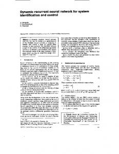
This section describes the proposed recurrent compensatory fuzzy neural network (RCFNN). Recently, Lin and Wai [8] proposed a model, called the recurrent fuzzy neural network (RFNN) architecture. The model presented here resembles the RFNN with the only difference being in the rule layer. Layer three of the RFNN uses the product operator, while layer three of the proposed model uses the compensatory operator. The structure of the proposed RCFNN is illustrated in Fig. 1, and is systematized into N input variables, R-term nodes for each input variable, M output nodes, and N×R membership function nodes. The RCFNN comprises four layers and R×(N×2+3+M) parameters, where R denotes the number of existing rules. Nodes in layer 1 are input nodes, which represent input variables. Moreover, nodes in layer 2 are called linguistic nodes and act as membership functions to express the input fuzzy linguistic variables. Nodes in this layer are used to calculate the Gaussian

Output layer W1 z-1

z-1

θ2

(9)

where mij and σij are, respectively, the mean and variance of the Gaussian membership function of the jth term of the ith input variable xi. Defining the number and the locations of the membership functions leads to a partition of the premise space ℵ = ℵ1 × ... ×ℵN . The collection of fuzzy sets Α j = {A1 j ,...,ANj } pertaining to the premise part of Rule-j forms a fuzzy region Aj that can be regarded as a multi-dimensional fuzzy set whose membership function is determined by N

μ A j ( x(t )) = ∏ μ Aij (xi (t )).

(10)

i =1

The above equation provides the degree to which a particular input vector x(t) belongs to the fuzzy region Aj. For the internal variable sj, the following sigmoid function is used: sj =

1 , 1 + exp{ − h j }

(11)

‧‧

‧‧

acting as memory elements, and θ j is the feedback

Rule layer

weight. Furthermore, due to the compensatory operation of the grades of the membership functions μ Aij (xi (t )) in (10), for simplicity, we can rewrite it

Linguistic laye

as:

W3

‧‧‧

‧‧ θ3

W2

z-1

⎧⎪ [xi − mij ]2 ⎫⎪ μ Aij ( xi ) = exp ⎨− ⎬, σ ij 2 ⎭⎪ ⎩⎪

where h j = μ A j ( x(t − 1)) ⋅ θ j is the feedback units

y

‧‧

membership values. Each node in layer 3 is called a compensatory rule node. Furthermore, nodes in layer 3 equal the number of compensatory fuzzy sets corresponding to each external linguistic input variable. Links before layer 3 represent the rule preconditions, and links after layer 3 represent the consequences of the rule nodes. Nodes in layer 4 are called output nodes, where each node represents an individual system output. The links between layers 3 and 4 are connected via the weighting values wj. Each node in the feedback layer is embedded in the RCFNN by adding feedback connections to layer 3. The structure of the RCFNN is shown in Fig. 1, in which Aij by a Gaussian-type membership function, μ Aij ( xi ) , defined by

(8)

3. STRUCTURE OF THE RECURRENT COMPENSATORY FUZZY NEURAL NETWORK

757

θ1

‧‧ h1(t)

h2(t)

Input layer

h3(t)

x1

x2

Fig. 1. Structure of the proposed RCFNN.

N

γ 1−γ j + j N

μ A j ( x(t )) = [∏ μ Aij ( xi ) ⋅ s j ]. i =1

(12)


758

Therefore, we can rewrite the fuzzy if-then rule as follows: Rule − j :[IF x1 (t ) is A1 j and ...... γj

and xN (t ) is ANj and h j (t ) is G ]

THEN y ′(t + 1) is w j and h j (t + 1) is θ j , (13) where Rule-j denotes the jth fuzzy rule, x(t)=[x1(t),x2(t),…,xN(t)]T is the input vector to the model at time t with xi (t ) ∈ℵi ⊂ ℜ(i = 1,..., N ),

h j (t ) is the internal variable at time t, y’(t+1) is the jth output of the local model for Rule-j, Aij and G are fuzzy sets, wj is the consequent part of Rule-j, and θ j is the fuzzy singleton. The output of the model at time t is y(t) and is labeled ∑. It is the sum of all incoming signals: R

y (t ) = ∑ μ A j (x(t )) ⋅ w j ,

(14)

j =1

where the weight wj is the output action strength of the output associated with the jth rule. Because (14) has a similar form to [16], which is a universal approximator, it is easy to prove the universal approximation theorem of (14), as follows. For any real continuous function g in a compact set U ⊂ ℜ N and for any given arbitrary ε > 0 , a model f exists such that sup f ( x) − g ( x) < ε . x∈U

Here • can be any norm. To summarize, the overall representation of the input x and the output y is γ 1−γ j + j

⎧ N ⎡ ( x (t ) − mij )2 ⎤ ⎫ ⎪ ∏ exp ⎢ − i ⎥ ⎪ R ⎪⎪ i =1 σ ij 2 ⎢⎣ ⎥⎦ ⎪⎪ y (t ) = ∑ w j ⋅ ⎨ ⎬ (3) ⎪1 + exp[−u j ( xi (t − 1)) ⋅ θ j ] ⎪ j =1 ⎪ ⎪ ⎪⎩ ⎪⎭, 2

(

2

where γ j = c j / c j + d j

2

)

N

(15)

Explicitly, using the RCFNN, the same inputs yield different outputs at different times. Obviously, (16) can be demonstrated to be a universal approximator by using the same method in [16].

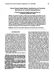
4. LEARNING ALGORITHMS OF RCFNN This section describes an on-line learning algorithm for constructing the RCFNN. The learning algorithm comprises both structure and parameter learning phases. Fig. 2 illustrates the flow diagram of the learning scheme for the RCFNN model. The structure learning algorithm is based on the measure of degree to determine the number of fuzzy rules. The parameter learning is based on supervised learning algorithms. Meanwhile, the gradient descent algorithm minimizes a given cost function by adjusting the weights in the consequent part, the weights of the feedback, the compensatory degree, and the parameters of the membership functions. Initially, the network contains no node except the input-output nodes; that is, there are no rules and memberships. The rule nodes are created dynamically and automatically as learning proceeds when online incoming training data are received and when the structure and parameter learning processes are performed. The details of the structure and parameter learning phases are described in the rest of this section. 4.1. Structure learning Structure learning initially attempts to determine whether to extract a new rule from the training data, and also to determine the number of fuzzy sets in the universal of discourse of each input variable, since one cluster in the input space corresponds to one potential fuzzy logic rule, with mij and σij representing the center and width, respectively, of the Gaussian membership function. For each incoming pattern x, the strength of rule firing can be interpreted as the degree to which the incoming pattern belongs to the corresponding cluster. To improve computational efficiency, a compensatory operator of the firing strength obtained from u (3) j ( x(t )) can be directly used as the degree measure

is the compensatory

degree, mij, σij, θj, cj, dj, and wj are the tuning parameters, and γ 1−γ j + j N

⎧ N ⎡ ( x (t − 1) − mij ) 2 ⎤ ⎫ ⎪ ∏ exp ⎢ − i ⎥⎪ 2 ⎪⎪ i =1 ⎢ ⎥ ⎪⎪ σ ij ⎣ ⎦ − = u (3) ( x ( t 1)) ⎨ ⎬ j (3) + − − ⋅ 1 exp[ u ( x ( t 2)) θ ⎪ i j]⎪ j ⎪ ⎪ ⎪⎩ ⎪⎭.

γ 1−γ j + j N

⎡ ⎡ n (2) ⎤ ⎤ = F j = u (3) ( x ( t )) ⎢ ⎢∏ uij ( xi ) ⎥ ⋅ s j ⎥ j ⎦⎥ ⎣⎢ ⎣⎢ i =1 ⎦⎥ ,

(17)

where F j ∈ [0,1] . Using this degree measure, the following criterion can be obtained for generating a new fuzzy rule for new incoming data, described as follows. Find the maximum degree Fmax Fmax =

(16)

max F , 1≤ j ≤ R(t ) j

(18)


where R(t) is the number of existing rules at time t. If Fmax ≤ F , then a new rule is generated, where F ∈ (0,1) is a prespecified threshold that should decay when the learning process limits the size of the RCFNN. We adopt the decay method (1 − i / N ) F , where N is the prespecified number of training epoch and i is ith training epoch when the learning process. The threshold parameter F is an important parameter in the structure learning step. The threshold value is set to between zero and one. A low threshold value leads to the learning of coarse clusters (that is, less rules are generated), whereas a high threshold value leads to the learning of fine clusters (that is, more rules are generated). If the threshold value equals zero, all the training data belong to the same cluster in the input space. After generating a new rule, the next step is to assign initial center and width according to (19) and (20) for the new Gaussian membership function. Since the goal of this study is to minimize an objective function, and since the center and width of Gaussian membership function are all adjustable later in the parameter learning, the center and width for the new Gaussian membership function are set as follows: ( R(t +1) )

= xi ,

(19)

( R( t +1) )

= σ init ,

(20)

mij

σ ij

where xi denotes the new data and σinit represents a prespecified constant. Therefore, the selection of the threshold value F and the prespecified constant σinit critically influence the simulation results, and the threshold value is based on practical experimentation or trial-and-error testing. Since the generation of a membership function corresponds to the generation of a new fuzzy rule, the ( R(t +1) )

compensatory degree c j (R ) γ j (t +1)

= (c j

( R( t +1) ) 2

) /(c j

( R(t +1) )

, dj

( R( t +1) ) 2

) + (d j

( R( t +1) )

weight of the feedback θ j the link

(R ) w j (t +1)

, namely,

( R(t +1) ) 2

) , the

, and the weight of

associated with a new fuzzy rule

have to be determined. Generally, the compensatory (R ) degree c j (t +1) (R ) θ j (t +1)

(R ) , d j (t +1) ,

the weight of the feedback ( R(t +1) )

, and the weight of the link w j

are

selected with random values in [-1,1]. The whole algorithm for the generation of new fuzzy rules as well as of fuzzy sets in each input variable is as follows. Suppose no rules initially exist: Step 1: IF xi is the first incoming pattern THEN do {Generate a new rule with center mi1=xi, width σi1=σinit, compensatory

759

degree c1=random, d1=random, weight of feedback θ1 = random , weight of link w1=random where σinit is a prespecified constant.} Step 2: ELSE for each newly incoming xi, do {Find Fmax = max F j 1≤ j ≤ R(t )

IF Fmax ≥ F do nothing ELSE { R(t+1) = R(t) +1 generate a new rule R

with center mij (t +1) = xi , width R

σ ij (t +1) = σ init , R

compensatory degree c j (t +1) = random , R

d j (t +1) = random, weight of feedback R

θ j (t +1) = random, weight of link R

w j (t +1) = random }

where σinit is a prespecified constant.}

4.2. Parameter learning body After adjusting the network structure based on the current training pattern, the network then enters the parameter learning phase to optimize the network parameters based on the same training pattern. Notice that the following parameter learning is performed on the whole network after structure learning, regardless of whether the nodes (links) are newly added or originally existed. Since the learning process involves the determination of the vector which minimizes a given cost function, the gradient of the cost function with respect to the vector is calculated, and the vector is adjusted along the negative gradient. When the single output case is considered for clarity, the goal is to minimize the cost function E(t), which is defined as 1 E (t ) = [ y d (t ) − y (t )]2 , 2

(21)

where yd(t) denotes the desired output and y(t) represents the current output for each discrete time t. During each training cycle, beginning at the input variables, a forward pass is used to calculate the activity of all the current outputs y(t). When the gradient descent learning algorithm is used, the weighting vector of the RCFNN is adjusted such that the error defined in (21) is below the desired threshold value after a given number of training cycles. The well-known gradient descent learning algorithm can be written briefly as

760


W (t + 1) = W (t ) + ΔW (t ) ⎛ ∂E (t ) ⎞ = W (t ) + η ⎜ − ⎟, ⎝ ∂W ⎠

(22)

where, in this case, η and W represent the learning rate and tuning parameters of the RCFNN, respectively. Let e(t ) = y (t )d − y (t ) and W = [m, σ ,θ , c, d , w]T represent the training error and weighting vector of the RCFNN, respectively. The gradient of error E(.) in (21) with respect to an arbitrary weighting vector W then is ∂E (t ) ∂y (t ) = −e(t ) . ∂W ∂W

⎡⎛ N ⎤ ⎞ ⋅ ⎢⎜ ∏ uij(2) ( xi ) ⎟ ⋅ s j ⎥ ⎟ ⎢⎣⎜⎝ i =1 ⎥⎦ ⎠

(23)

The error term for each layer is first computed to form recursive applications of the chain rule. The parameters in the corresponding layers then are adjusted. With the RCFNN and the cost function as defined in (21), the update rule for wj, cj, dj, and θ j

= (1 − γ j +

∂E (t ) , ∂w j

(24)

∂E (t ) c j (t + 1) = c j (t ) − ηc , ∂c j

(25)

∂E (t ) d j (t + 1) = d j (t ) − ηd , ∂d j

(26)

∂E (t ) θ j (t + 1) = θ j (t ) − ηθ , ∂θ j

(27)

N

)

⎡⎛ N ⎤ ⎞ ⋅ ⎢⎜ ∏ uij(2) ( xi ) ⎟ ⋅ s j ⎥ ⎟ ⎢⎣⎜⎝ i =1 ⎥⎦ ⎠

γ −γ j + j N

(

)

⋅ s j ⋅ 1− s j ⋅

∂h j ∂θ j

and the partial derivative ∂h j ∂θ j is calculated as ∂h j ∂s j (3) (2) = u j (t − 1) + θ j ⋅ (t − 1) ⋅ uij (t − 1). ∂θ j ∂θ j Hence, we have the following recursive form: ∂s j (t ) = s j (t ) ⋅ 1 − s j (t ) ⋅ ∂θ j

(

)

⎡ (3) ⎤ ∂s j (2) ⎢u j (t − 1) + θ j ⋅ uij (t − 1) ⋅ (t − 1) ⎥ . ∂θ j ⎢⎣ ⎥⎦

can be derived, as follows: w j (t + 1) = w j (t ) − η w

γj

γ −γ j + j N ∂s j ⋅ ∂θ j

Similarly, the update laws for mij and σ ij are mij (t + 1) = mij (t ) − ηm

∂E (t ) , ∂mij

(28)

σ ij (t + 1) = σ ij (t ) − ησ

∂E (t ) , ∂σ ij

(29)

where

where ∂E (t ) = −e(t ) ⋅ u (3) j ( x(t )), ∂w j ∂E (t ) = −e(t ) ⋅ w j ⋅ u (3) j ( x(t )) ∂c j ⎡N ⎤ ⎛1 ⎞ ⎡ 2c(t )d 2 (t ) ⎤⎥ , ⋅ln ⎢ ∏ uij(2) ( xi ) ⋅ s j ⎥ ⋅ ⎜ − 1⎟ ⋅ ⎢ ⎠ ⎢⎣ (c 2 (t ) + d 2 (t ))2 ⎥⎦ ⎣⎢i =1 ⎦⎥ ⎝ N ∂E (t ) = −e(t ) ⋅ w j ⋅ u (3) j ( x(t )) ∂d j ⎡N ⎤ ⎛1 2c2 (t )d (t ) ⎤⎥ ⎞ ⎡ , ⋅ln ⎢ ∏ uij(2) ( xi ) ⋅ s j ⎥ ⋅ ⎜ − 1⎟ ⋅ ⎢ − ⎠ ⎣⎢ (c 2 (t ) + d 2 (t ))2 ⎦⎥ ⎢⎣i =1 ⎥⎦ ⎝ N (3) ∂u (3) ∂E (t ) ∂y ∂u j j , = −e(t ) ⋅ ⋅ = −e(t ) ⋅ w j ⋅ (3) θ θ ∂θ j ∂ ∂ j j ∂u j where ∂u (3) γj j = (1 − γ j + ) ∂θ j N

(3) (3) ∂u j ∂E (t ) ∂y ∂u j , = −e(t ) ⋅ ⋅ = −e(t ) ⋅ w j ⋅ (3) ∂mij ∂mij ∂mij ∂u j (3) (3) ∂u j ∂E (t ) ∂y ∂u j , = −e(t ) ⋅ ⋅ = −e(t ) ⋅ w j ⋅ (3) ∂σ ij ∂σ ij ∂σ ij ∂u j

where ∂u (3) j

⎧⎡

⎡

(

⎢ xi − mij ∂ ⎪⎪ ⎢ N = ⎨ ⎢ ∏ exp ⎢ − ∂mij ∂mij ⎪ ⎢i =1 ⎢ σ ij2 ⎢⎣ ⎪⎢ ⎩⎣

⎛

= ⎜⎜1 − γ j + ⎝

)

2 ⎤⎤

γ 1−γ j + j ⎫ N

⎥⎥ ⎪⎪ ⎥⎥ ⋅ s j ⎬ ⎥⎥ ⎪ ⎥⎦ ⎥⎦ ⎪⎭

γ −γ j + j ⎤ N

γ j ⎞ ⎡⎛ N (2) ⎞ ⎟ ⋅ ⎢⎜ ∏ uij ⎟ ⋅ s j ⎥ ⎟ N ⎠ ⎢⎣⎜⎝ i =1

(

⎧ ⎡ ⎪ ⎡ N (2) ⎤ ⎢ 2 ⋅ xi − mij ⋅ ⎨ ⎢ ∏ uij ⎥ ⋅ ⎢ ⎥⎦ ⎢ ⎪ ⎢⎣i =1 σ ij2 ⎣ ⎩

⎟ ⎠

) ⎤⎥ ⋅ s ⎥ ⎥ ⎦

⎥⎦ ⎫

∂s j ⎡ N (2) ⎤ ⎪ j + ∂m ⋅ ⎢ ∏ uij ⎥ ⎬ ⎥⎦ ⎪ ij ⎢⎣i =1 ⎭

and the partial derivative ∂s j ∂mij is calculated as


∂s j ∂mij

(

)

= sj ⋅ 1− sj ⋅

∂h j ∂mij

(

= sj ⋅ 1− sj

5. SIMULATION RESULTS

)

⎧⎪ ⎡ ∂s j ⋅ ⎨θ j ⋅ ⎢ (t − 1) ⋅ uij(2) (t − 1) ∂ m ⎣⎢ ij ⎩⎪

(

⎡ 2 ⋅ xi − mij + s j (t − 1) ⋅ uij(2) (t − 1) ⋅ ⎢ ⎢ σ ij2 ⎣

) ⎤⎥ ⎤⎥ ⎪⎫

⎬ ⎥⎥⎪ ⎦⎦⎭

and γ 1−γ j + j N ⎧⎡ 2 ⎤⎤ ⎫ ⎡ (3) ∂u j ⎪⎪ ⎢ xi − mij ⎥ ⎥ ∂ ⎪⎪ ⎢ N = ⎨ ⎢ ∏ exp ⎢ − ⎥⎥ ⋅ s j ⎬ ∂σ ij ∂σ ij ⎪ ⎢i =1 σ ij2 ⎪ ⎢ ⎥⎥ ⎣ ⎦ ⎥⎦ ⎪⎩ ⎢⎣ ⎪⎭ γ −γ + j γ j ⎞ ⎡⎛ N (2) ⎞ ⎛ ⎤ j N ⎧⎪ ⎡ N (2) ⎤ = ⎜1 − γ j + ⋅ ⎨ ⎢ ∏ uij ⎥ ⎟ ⋅ ⎢⎜ ∏ u ⎟ ⋅ s ⎥ ⎜ N ⎟⎠ ⎣⎝ i =1 ij ⎠ j ⎦ ⎦ ⎩⎪ ⎣i =1 ⎝

(

2⎤ ⎡ ∂s j ⎢ 2 ⋅ xi − mij ⎥ ⋅⎢ ⋅sj + ⎥ ∂σ ij σ ij3 ⎢ ⎥ ⎣ ⎦

(

)

)

⎫ ⎡ N (2) ⎤ ⎪⎪ ⋅ ⎢ ∏ uij ⎥ ⎬ ⎣i =1 ⎦⎪ ⎪⎭

∂σ ij

(

)

= sj ⋅ 1− sj ⋅

∂h j ∂σ ij

(

= s j ⋅ 1− s j

)

+ s j (t

(

⎡2⋅ x − m i ij − 1). ⎢ 3 ⎢ σ ij ⎣⎢

5.1. Identification of dynamic system The systems to be identified are dynamic systems whose outputs are functions of past inputs and outputs. For this dynamic system identification, since a recurrent network is used, only the current states of the system and control signal are used as network inputs. The model is applied in the following two identification problems.

where f ( x1 , x2 , x3 , x4 , x5 ) =

⎡ ∂s j ⎪⎧ ⋅ ⎨θ j ⋅ ⎢ (t − 1) ⋅ uij(2) ∂ σ ⎢⎣ ij ⎪⎩ − 1) ⋅ uij(2) (t

This study evaluated the performance of the RCFNN for temporal problems. This section presents several examples and performance contrasts with some other recurrent fuzzy neural networks. The first problem involves identifying a nonlinear dynamic system, while the second problem involves identifying a chaotic system. In the following simulations, the parameters and number of training epochs were determined based on the desired result.

Example 1: In this example, a nonlinear plant with multiple time delays was guided using the following differential equation: y p (t + 1) = f ( y p (t ), y p (t − 1), (30) y p (t − 2), u p (t ), u p (t − 1)),

and the partial derivative ∂s j ∂σ ij is ∂s j

761

)

2

⎤⎤⎫ ⎥⎥⎪ ⎥⎥⎬ ⎪ ⎦⎥ ⎥⎦ ⎭.

Fig. 2. Flow diagram of the structure/parameter learning for the RCFNN model.

x1 x2 x3 x5 ( x3 − 1) + x4

. 1 + x2 2 + x32 In this study, the current output of the plant depends on three previous outputs and two previous inputs. In [6], the feedforward neural network, with five input nodes for feeding, the appropriate past values of yp and u were used. In the proposed model, only two input values, yp(t) and u(t), were fed to the RCFNN to determine the output yp(t+1). The training inputs were independent and had an identically distributed (i.i.d.) uniform sequence over [-2,2] for about half of the training time and a single sinusoid signal given by 1.05sin(πt/45) for the remainder of the training time. These 900 training data were not repeated; that is, different training sets were used for each epoch. The test input signal u(t), as shown in the equation below, was used to determine the identification results. ⎧ ⎛π ⋅t ⎞ 0 < t < 250 ⎪ sin ⎜ 25 ⎟ ⎝ ⎠ ⎪ ⎪ 1.0 250 ≤ t < 500 ⎪ 500 ≤ t < 750 ⎪ −1.0 u (t ) = ⎨ ⎪0.3sin ⎛ π ⋅ t ⎞ + 0.1sin ⎛ π ⋅ t ⎞ ⎜ ⎟ ⎜ ⎟ ⎪ ⎝ 25 ⎠ ⎝ 32 ⎠ ⎪ ⎪ +0.6sin ⎛ π ⋅ t ⎞ 750 ≤ t < 1000. ⎜ ⎟ ⎪ ⎝ 10 ⎠ ⎩

762


Ten epochs were used for training the RCFNN. The learning rateηw=ηc=ηd=ηm=ησ=ηθ=0.05, the prespecified σinit = 0.2, and the prespecified threshold F = 10−4 were chosen. After training, the final rootmean-square error (rms error) was 0.0011, and three fuzzy logic rules were generated. These designed three fuzzy IF-THEN rules of the recurrent compensatory fuzzy neural network with a compensatory degree γ are described below Rule 1: IF [ u(t) is μ(-0.0313,0.3149) and y(t) is μ(0.1539, 0.7908) and h(t) is G]0.3724 THEN y(t+1) is 0.4686 and h(t+1) is 0.4686 Rule 2: IF [ u(t) is μ(0.6041,0.3120) and y(t) is μ(1.0319, 0.4989) and h(t) is G]0.7094 THEN y(t+1) is 0.9018 and h(t+1) is-0.5938 Rule 3: IF [ u(t) is μ(-1.3234,0.6565) and y(t) is μ(-1.1754, 0.7360) and h(t) is G]0.9352 THEN y(t+1) is –1.3784 and h(t+1) is 0.0816 Fig. 3(a) shows the distribution of some of the training patterns and the final assignment of the rules in the [u(t),y(t)] plane. This is due to the parameter learning process, which adjusts the center and width of each Gaussian membership function at each time step to minimize the output cost function. Fig. 3(a) shows the membership functions in the u(t) and y(t) dimensions. Moreover, Fig. 3(b) illustrates the distribution of the testing patterns on the y(t) and u(t) dimensions. Additionally, Fig. 3(c) shows results using the RCFNN for identification. The analytical results demonstrate that the RCFNN model can achieve perfect identification. Fig. 3(d) illustrates the error between the desired output and the RCFNN output. Moreover, Fig. 3(e) shows the learning curves of the RCFNN, RSONFIN [7], RFNN [8], and TRFNS [9] models. In the figure, the proposed model converges faster than other models. In many practical cases, the plant being identified is noisy. Internal plant noise appears at the plant output and is commonly represented as an additive noise. In the present simulations, noise is white Gaussian distributed with σ e2 = 0.1 . Fig. 4(a) plots the noise-corrupted signal. Moreover, Fig. 4(b) shows a trace of the recovered signal sequence. This study also compared the performance of the proposed model with that of other existing recurrent methods (RSONFIN [7], RFNN [8], TRFN-S [9]). The performance indices considered included the numbers of adjustable parameters, the rms error (training and testing), and the numbers of epochs. Table 1 lists the comparison results. As listed in Table 1, the numbers of adjustable parameters and the rms error of the RCFNN are smaller than other recurrent

(a) The input training patterns and the final assignment of rules for the distribution of the membership functions on the y(t) and u(t) dimensions.

(b) The distribution of the testing patterns on the y(t) and u(t) dimensions.

(c) The outputs of the plant and the RCFNN.

(d) The error between the RCFNN output and the desired output.

(e) The learning curves of the RCFNN, RSONFIN [7], the RFNN [8] and the TRFN-S [9]. Fig. 3. Simulation results of the RCFNN for dynamic system identification in Example1.


763

μ(0.0115,0.2374) and h(t) is G]0.4192 THEN y(t+1) is 0.4047 and h(t+1) is 0.5621 Rule 2: IF [u(t) is μ(0.9473,-0.4273) and y(t) is μ(1.0411,1.1604) and h(t) is G]0.9466 THEN y(t+1) is 1.0166 and h(t+1) is 0.4766

(a) The noise-corrupted signal.

Rule 3: IF [u(t) is μ(-0.7305,0.3594) and y(t) is μ(-0.8313,0.8858) and h(t) is G]0.9504 THEN y(t+1) is –0.7550 and h(t+1) is 0.7186

(b) Output of the plant and the identification RCFNN for the same input. Fig. 4. Simulation results in the noisy case of the RCFNN for dynamic system identification. Table 1. Performance comparison of various recurrent methods with respect to the identification problem in Example 1. RCFNN Parameters

24

RMS error 0.0011 (training) RMS error 0.0019 (testing) Epochs

10

RSONFIN RFNN [7] [8]

TRFN-S [9]

36

24

33

0.0248

0.0030

0.0084

0.0780

0.0033

0.0346

10

10

10

models under the same training epochs. Example 2: Next consider the following dynamic plant with longer input delays: y p (t + 1) = 0.72 y p (t ) + 0.025 y p (t − 1)u (t − 1) + 0.01u 2 (t − 2) + 0.2u (t − 3).

(31)

This plant is the same as that used in [17]. The current output of the plant depends on two previous outputs and three previous inputs. As in example 1, the identification model, where only two external input values were fed to the input of RCFNN. The training data and time steps were the same as in Example 1. Ten epochs were used in training the RCFNN. The learning rateηw=ηc=ηd=ηm=ησ =ηθ=0.05, the prespecified σinit = 0.2, and the prespecified threshold F = 10−4 were chosen. After training, the final rms error was 0.0005, and three fuzzy logic rules were generated. These designed three rules with a compensatory degree are Rule 1: IF [u(t) is μ(0.1786,0.4733) and y(t) is

The check signal used in Example 1 is adopted for checking the identified result. Fig. 5(a) shows the distribution of input training patterns and the final task of the rules in the [u(t),y(t)] plane. Fig. 5(a) shows the membership functions in the u(t) and y(t) dimensions. Moreover, Fig. 5(b) shows the distribution of the testing patterns in the y(t) and u(t) dimensions. Additionally, Fig. 5(c) shows the outputs of the plant and the RCFNN for the testing patterns. The analytical results also show the perfect identification capability of the RCFNN model. Moreover, Fig. 5(d) illustrates the error between the desired output and the RCFNN output. Meanwhile, Fig. 5(e) shows the learning curve of the RCFNN, the RSONFIN [7], the RFNN [8], and the TRFN-S [9]. Simultaneously, the plant additive noise was also identified by RCFNN. Fig. 6(a) illustrates the corrupted signal. Finally, Fig. 6(b) shows the recovered signal using the RCFNN after convergence. This study compared the performance of the proposed model with that of other existing recurrent methods (RSONFIN [7], RFNN [8], and TRFN-S [9]). This study demonstrates that the proposed network outperforms its comparing rivals, and exhibits a smaller rms error for the same learning epochs. We can find that the required parameters of the proposed method are less than the parameter number of the other methods. Obviously, as shown in Table 2, the RCFNN is more effective than other existing recurrent networks. 5.2. Identification of a chaotic system This subsection discusses a typical discrete time chaotic system, which is easier to describe. Successful simulation results are then presented by training the RCFNN model. Performance comparisons with the FNN [5], RSONFIN [7], RFNN [8], and TRFN-S [9] are presented in this subsection to verify the performance of the RCFNN for temporal problems. Example 3: The discrete time Henon system is repeatedly used in the study of chaotic dynamics and is not too simple in the sense that it is of the second order with one delay and two parameters [18]. This chaotic system is described by

764


(a) The corrupted signal.

(a) The input training patterns and final assignment of rules for the distribution of the membership functions on the y(t) and u(t) dimensions.

(b) Output of the plant and the identification RCFNN. Fig. 6. Simulation results in the noisy case of the RCFNN for nonlinear system identification. Table 2. Performance comparison of various recurrent methods with respect to the identification problem in Example 2. RCFNN Parameters

(b) The distribution of the testing patterns on the y(t) and u(t) dimensions.

RMS error (training) RMS error (testing) Epochs

(c) The outputs of the plant and the RCFNN.

(d) The error between the RCFNN output and the desired output.

(e) Learning curve of the RCFNN, the RSONFIN [7],the RFNN [8] and the TRFN-S [9]. Fig. 5. Simulation results of the RCFNN for nonlinear system identification in Example2.

RSONFIN RFNN TRFN-S [7] [8] [9]

24

49

24

33

0.0005

0.0300

0.0014

0.0067

0.0015

0.0600

0.0026

0.0313

10

10

10

10

y (t + 1) = − P ⋅ y 2 (t ) + Q ⋅ y (t − 1) + 1.0, for t = 1, 2,...,

(32)

which, with P=1.4 and Q=0.3, produces a chaotic strange attractor, as shown in Fig. 7(a). For this training, the input of the RCFNN was y(t-1) and the output was y(t). We first randomly took the training data (1000 pairs) from a system over the interval [1.5,1.5]. Then the RCFNN was used to approximate the chaotic system. In applying the RCFNN to this example, this study used only 100 epochs. Here, the initial point was [y(1),y(0)]T=[0.4,0.4]T. The learning rateηw=ηc=η d=ηm=ησ=ηθ=0.05, the prespecified σinit=0.1, and the prespecified threshold F = 10−4 were chosen. After training, eight fuzzy logic rules were generated. The phase plane of this chaotic system after training for the FNN [5] and the RCFNN are shown in Fig. 7(b) and Fig. 7(c), respectively. Simulation results in Fig, 7(b), indicate that the FNN is inappropriate for chaotic dynamics system because of its static mapping.


765

proposed model is smaller than the RSONFIN model [7], the RFNN model [8], the TRFN-S model [9] and the FNN model [5] under the same fuzzy rules and training epochs.

6. CONCLUSIONS

(a) The testing data of this chaotic system.

(b) Result of identification using the FNN for the chaotic system.

This study presents a recurrent compensatory fuzzy neural network for identifying dynamic systems. The RCFNN is a recurrent multilayered connectionist network for realizing fuzzy inference using dynamic fuzzy rules. The network comprises four layers, including two hidden layers and a feedback network. An on-line learning algorithm that consists of structure learning and parameter learning is also proposed to automatically construct the RCFNN. The structure learning algorithm is based on the measure of degree and determines whether or not to add a new node to satisfy the fuzzy partition of the input data. Moreover, the gradient descent learning algorithm is used for tuning input membership functions. Simulation results demonstrate the effectiveness of the proposed RCFNN model in resolving many temporal problems. [1] [2]

(c) Result of identification using the RCFNN for the chaotic system.

[3]

Fig. 7. Simulation results for identification of a chaotic system.

[4]

Table 3. Performance comparison of various methods with respect to the chaotic system identification problem in Example 3.

[5]

RCFNN Number of 8 rules RMS error 0.0034 (train) RMS error 0.0036 (test) Epochs

100

RSONFIN RFNN TRFN- FNN [7] [8] S [9] [5] 8

8

8

8

[6]

0.0755 0.0141 0.0306 0.1338 0.0927 0.0145 0.0341 0.1577 100

100

100

[7]

100

The comparison of performance in Table 3 reveals that the rms error (training and testing) of the

[8]

REFERENCES C. T. Lin and C. S. G. Lee, Neural Fuzzy Systems: A Neuro-Fuzzy Synergism to Intelligent System, Prentice-Hall, NJ, 1996. J. S. R. Jang, “ANFIS: Adaptive-network-based fuzzy inference system,” IEEE Trans. on Systems, Man, and Cybernetics, vol. 23, no. 3, pp. 665-685, 1993. C. J. Lin and C. T. Lin, “Reinforcement learning for an ART-based fuzzy adaptive learning control network,” IEEE Trans. Neural Networks, vol. 7, pp. 709-731, June 1996. C. F. Juang and C. T. Lin, “An on-line selfconstructing neural fuzzy inference network and its applications,” IEEE Trans. on Fuzzy Systems, vol. 6, no. 1, pp. 12-31, Feb. 1998. F. J. Lin, C. H. Lin, and P. H. Shen, “Selfconstructing fuzzy neural network speed controller for permanent-magnet synchronous motor drive,” IEEE Trans. on Fuzzy Systems, vol. 9, pp. 751-759, Oct. 2001. K. S. Narendra and K. Parthasarathy, “Identification and control of dynamical systems using neural networks,” IEEE Trans. on Neural Networks, vol. 1, pp. 4-27, 1990. C. F. Juang and C. T. Lin, “A recurrent selforganizing neural fuzzy inference network,” IEEE Trans. on Neural Networks, vol. 10, no. 4, pp. 828-845, July 1999. F. J. Lin and R. J. Wai, “Hybrid control using recurrent fuzzy neural network for linearinduction motor servo drive,” IEEE Trans. on

766

[9]

[10] [11]

[12]

[13]

[14]

[15]

[16]

[17]

[18]


Fuzzy Systems, vol. 9, no. 1, pp. 102-115, Feb. 2001. C. F. Juang, “A TSK-type recurrent fuzzy network for dynamic systems processing by neural network and genetic algorithms,” IEEE Trans. on Fuzzy Systems, vol. 10, no. 2, pp. 155170, Apr. 2002. H. J. Zimmermann and P. Zysno, “Latent connective in human decision,” Fuzzy Sets and Systems, vol. 4, pp. 37-51, 1980. Y. Q. Zhang and A. Kandel, “Compensatory neurofuzzy systems with fast learning algorithms,” IEEE Trans. on Neural Networks, vol. 9, no. 1, pp. 83-105, Jan. 1998. M. Mizumoto, “Pictorial representations of fuzzy connectives, part II: Cases of compensatory operators and self-dual operators,” Fuzzy Sets and Systems, vol. 32, pp. 45-79, 1989. H. Seker, D. E. Evans, N. Aydin, and E. Yazgan, “Compensatory fuzzy neural networks-based intelligent detection of abnormal neonatal cerebral doppler ultrasound waveforms,” IEEE Trans. on Information Technology in Biomedicine, vol. 5, no. 3, pp. 187-194, 2001. C. J. Lin and C. H. Chen, “Nonlinear system control using compensatory neuro-fuzzy networks,” IEICE Fundamentals on Electronics, Communications and Computer Sciences, vol. E86-A, no. 9, pp. 2309-2316, 2003. C. J. Lin and W. H. Ho, “A pseudo-gaussianbased compensatory neural fuzzy system,” Proc. of the IEEE International Conference on Fuzzy Systems, St. Louis, MO, USA, pp. 214-220, May 25-28, 2003. C. J. Lin and C. C. Chin, “Prediction and identification using wavelet-based recurrent fuzzy neural networks,” IEEE Trans. on Systems, Man, and Cybernetics, vol. 34, no. 5, pp. 21442154, Oct. 2004. J. H. Kim and U. Y. Huh, “Fuzzy model based predictive control,” Proc. of IEEE Int. Conf. Fuzzy Systems, vol. 1, Anchorage, AK, pp. 405409, May 1998. G. Chen, Y. Chen, and H. Ogmen, “Identifying chaotic systems via a wiener-type cascade model,” IEEE Control Systems Magazine, vol. 17, no. 5, pp. 29-36, Oct. 1997. Chi-Yung Lee received the B.S. degree in Electronic Engineering from the National Taiwan University of Science and Technology, Taiwan, R.O.C., in 1981 and the M.S. degree in Industrial Education from the National Taiwan Normal University, Taiwan, R.O.C., in 1989. From August 1989 to July 2004, he was a Lecturer in the

Department of Electronic Engineering, Nan-Kai Institute of Technology, Nantou, Taiwan, R.O.C. Since August 2004, he has been with the Department of Computer Science and Information Engineering, Nan-Kai Institute of Technology. Currently, he is an Associate Professor of Computer Science and Information Engineering Department, Nan-Kai Institute of Technology, Nantou, Taiwan, R.O.C. His current research interests are neural networks, fuzzy systems, intelligence control, and FPGA design. Cheng-Jian Lin received the B.S. degree in Electrical Engineering fromTa-Tung University, Taiwan, R.O.C., in 1986 and the M.S. and Ph.D. degrees in Electrical and Control engineering from the National ChiaoTung University, Taiwan, R.O.C., in 1991 and 1996. From April 1996 to July 1999, he was an Associate Professor in the Department of Electronic Engineering, Nan-Kai College, Nantou, Taiwan, R.O.C. From August 1999 to January 2005, he was an Associate Professor in the Department of Computer Science and Information Engineering, Chaoyang University of Technology. From February 2005 to July 2007, he was a full Professor in the Department of Computer Science and Information Engineering, Chaoyang University of Technology. Currently, he is a full Professor of Electrical Engineering Department, National University of Kaohsiung, Kaohsiung, Taiwan, R.O.C. His current research interests are soft computing, pattern recognition, intelligent control, image processing, bioinformatics, and FPGA design. Cheng-Hung Chen was born in Kaohsiung, Taiwan, R.O.C. in 1979. He received the B.S. and M.S. degrees in Computer Science and Information Engineering from the Chaoyang University of Technology, Taiwan, R.O.C., in 2002 and 2004. He is currently working toward a Ph.D. degree in Electrical and Control Engineering at National Chiao-Tung University, Taiwan, R.O.C. His current research interests are neural networks, fuzzy systems, evolutionary algorithms, intelligent control, and pattern recognition. Chun-Lung Chang received the B.S. degree in Automatic Control Engineering from the Feng-Chia University, Taichung, Taiwan, in 1990, and the M.S. degree in Power Mechanical Engineering from the National TsingHua University, Hsinchu, Taiwan, in 1992, and the Ph.D. degree in Electrical and Control Engineering at National Chiao-Tung University, Taiwan, in 2006. He is a Researcher and Manager in Mechanical and Systems Research Laboratories, Industrial Technology Research Institute, Hsinchu, Taiwan. His current research interests are computer vision, pattern recognition, neural networks, and fuzzy inference system.