Dynamic Non-singleton Fuzzy Logic Systems For ... - Semantic Scholar

IEEE TRANSACTIONS ON FUZZY SYSTEMS, VOL. 5, NO. 2, MAY 1997

199

Dynamic Non-Singleton Fuzzy Logic Systems for Nonlinear Modeling George C. Mouzouris and Jerry M. Mendel, Fellow, IEEE

Abstract—We investigate dynamic versions of fuzzy logic systems (FLS’s) and, specifically, their non-Singleton generalizations (NSFLS’s), and derive a dynamic learning algorithm to train the system parameters. The history-sensitive output of the dynamic systems gives them a significant advantage over static systems in modeling processes of unknown order. This is illustrated through an example in nonlinear dynamic system identification. Since dynamic NSFLS’s can be considered to belong to the family of general nonlinear autoregressive moving average (NARMA) models, they are capable of parsimoniously modeling NARMA processes. We study the performance of both dynamic and static FLS’s in the predictive modeling of a NARMA process. Index Terms—Dynamic NSFLS, NARMA, nonlinear modeling.

I. INTRODUCTION

P

ROMPTED BY the desire to bridge the gap between traditional mathematical models of physical processes and the often abstract, or imprecise information associated with such processes, researchers in recent years have started paying particular attention to fuzzy set theory [29], a mathematical tool for translating abstract concepts into computable entities [4]. In this paper, we present computational systems capable of processing such entities. In Section II, we give a brief overview of non-Singleton fuzzy logic systems (NSFLS’s) [14], [15] that are an extension of the well-known Singleton fuzzy logic systems [9], [25]. These systems implement static nonlinear mappings between their input and output spaces. Here, we extend these systems to their dynamic feedback counterparts. The output of dynamic systems at time depends on exogenous inputs as well as previous outputs at time so these systems exhibit rich and complex dynamical behavior and can be used to parsimoneously represent dynamic processes of unknown order and structure. Unlike static fuzzy logic systems (FLS’s), processing of input patterns by dynamic FLS’s depends upon the order of presentation during training or recall; therefore, dynamic FLS’s are well suited for the representation and processing of temporal information. In Section III we derive a dynamic backpropagation type of learning algorithm to update the parameters of a dynamic non-Singleton fuzzy logic system. Although it was a long time after its inception (see [26]) that attention was drawn Manuscript received December 20, 1995; revised September 5, 1996. This work was supported by the University of Southern California, Los Angeles, National Science Foundation under Grant MIP-9 122 018. The authors are with the Signal and Image Processing Institute, Department of Electrical Engineering-Systems, University of Southern California, Los Angeles, CA 90089 USA. Publisher Item Identifier S 1063-6706(97)02843-9.

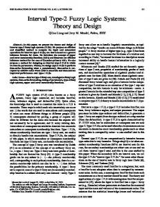
to backpropagation learning, its utility as a universal learning paradigm for smooth parameterized models (including FLS’s) [8], [15], [23] became evident with its successful application to artificial neural networks [17]. Being able to utilize a learning algorithm such as backpropagation implies that a FLS with linguistic information in its rulebase can be updated or adapted using numerical information to gain an even greater advantage over a neural network that cannot make direct use of linguistic information. The collection of modifiable IF-THEN rules comprising the rulebase, constitute an adaptive FLS, i.e., a system whose input–output behavior is defined by a set of modifiable parameters. The systems we describe in this paper belong to the family of adaptive FLS’s. In Section IV we give examples in system identification and the predictive modeling of a nonlinear autoregressive moving average process. These examples illustrate the power of both the dynamic FLS’s, and the dynamic learning algorithm. Section V concludes this paper. II. OVERVIEW OF NON-SINGLETON FUZZY LOGIC SYSTEMS The large variety of possible available information, together with the need for modeling all such information to determine a particular solution, necessitate the use of a very flexible information modeling technique. With this in mind, the formulation that provides the highest degree of latitude is a list of statements (rules) where each statement indicates the acceptability of a proposed solution based on some piece of information. The fuzzy formalism can provide a general framework to model certain or uncertain information in which an action is combined with a statement in an antecedent/consequent format and the individual statement solutions are aggregated to provide the overall solution. The set of statements comprise the fuzzy rule base, which is a vital part of a FLS (Fig. 1). The fuzzy inference engine combines the statements in the rule base according to approximate reasoning theory to produce a mapping from fuzzy sets in the input space to fuzzy sets in the output space The fuzzifier maps crisp inputs to fuzzy sets defined on the input space and the defuzzifier maps the aggregated output fuzzy sets to a single crisp point in the output space. A fuzzy logic system processes crisp data at the input and produces crisp data at the output; therefore, a fuzzifier is used at the front of the system to convert crisp data to fuzzy data and a defuzzifier is used at the output of the system to convert fuzzy data into crisp data. The most widely used fuzzifier is the Singleton fuzzifier [9], [10], [25], mainly because of its simplicity and lower computational requirements; however,

1063–6706/97$10.00  1997 IEEE

200


Fig. 1. Structure of a fuzzy logic system.

this kind of fuzzifier may not always be adequate, especially in cases where noise is present in the training data or in the data which is later processed by the system. A different approach is necessary to account for uncertainty in the data, which is why we direct our attention at NSFLS’s. NSFLS’s are a family of systems that have non-Singleton fuzzy sets as inputs. The structure of the rulebase is identical as in the Singleton FLS case, except that input linguistic variables are allowed to take set values (instead of single-point values). NSFLS’s are a powerful generalization of Singleton FLS’s and provide a mathematically tractable method to treat input uncertainty. Non-Singleton fuzzifiers have been used successfully in a variety of applications [1], [5], [16], [19], [20], [22]. In neuralfuzzy systems [1], [5], vectors of fuzzy sets are used both to train a fuzzy neural network and as inputs during processing. In [16], an optimizing control method for optimizing the fuel consumption rate of a marine diesel engine utilizes empirical rules that are expressed by fuzzy numbers. Non-Singleton input has also been used in turning process automation [20] to represent a human operator’s actions in the fuzzy rule base, in the design of fuzzy control algorithms [19], and in fuzzy information and decision-making [22]. These methods are largely heuristic and provide no closed-form expressions for fuzzy logic systems; hence, their generalizations are very difficult.

2) In the case of a non-Singleton fuzzifier, the point is mapped into a fuzzy set with support where achieves maximum value at and decreases while moving away from . We assume that fuzzy set is normalized so that Non-Singleton fuzzification is especially useful in cases where the available training data or the input data to the fuzzy logic system are corrupted by noise. Conceptually, the nonSingleton fuzzifier implies that the given input value is the most likely value to be the correct one from all the values in its immediate neighborhood; however, because the input is corrupted by noise, neighboring points are also likely to be the correct values, but to a lesser degree. It is up to the system designer to determine the shape of the membership function based on an estimate of the kind and quantity of noise or uncertainty present. It would be the logical choice, though, for the membership function to be symmetric about since the effect of noise is most likely to be equivalent on all points. Examples of such membership functions are: 1) the Gaussian

where the variance 2) triangular

reflects the width (spread) of

;

A. The Non-Singleton Fuzzifier Fuzzy sets have been interpreted as membership functions [29] that associate with each element of the universe of a number in the interval [0, 1]: discourse,

and 3)

(1) into a fuzzy set A fuzzifier maps a crisp point 1) In the case of a Singleton fuzzifier, the crisp point is mapped into a fuzzy set with support where for and for , i.e., the single point in the support of with nonzero membership function value is

where and are, respectively, the mean and spread of the fuzzy sets. Note that larger values of the spread of the above membership functions imply that more noise is anticipated to exist in the given data.

MOUZOURIS AND MENDEL: DYNAMIC NON-SINGLETON FUZZY LOGIC SYSTEMS

201

B. Dynamic Non-Singleton Fuzzy Logic System Formulation rules, Consider a fuzzy logic system with a rulebase of and let the th rule be denoted by Let each rule have antecedents and one consequent (as is well known, a rule with consequents can be decomposed into rules, each having the same antecedents and one different consequent); also, let and denote the antecedent membership functions corresponding to exogenous inputs and feedback inputs, respectively. For example, in the case of a single-feedback input, and the feedback input linguistic variable takes system output values delayed by one unit. The th rule is of the general form IF

is

and is

and and

THEN

and

is

and

is

is

where and are the input and output linguistic variables, respectively. Each and are subsets of possibly different universes of discourse. Let

(3) where and

are the fuzzy sets describing the exogenous and feedback inputs, respectively. Up to this point, the formulation is identical to that of the Singleton case. In the Singleton case, though, it is assumed that each input fuzzy set has nonzero membership value only at a single point, which reduces to a set with a single point In our treatment here, we do not make this assumption. Each input fuzzy set is represented by the more general nonSingleton form in (3), thereby allowing any uncertainty in the input to be represented in the system. According to the compositional rule of inference, the fuzzy subset of induced by is given by the composition of and (4)

and

in and over Note that all unions (denoted by are over the same spaces; therefore, we can write as

Since are feedback input linguistic variables, they take values from universe of discourse ; thus, (to maintain consistent notation with the antecedent linguistic variables, we will use to denote universes of discourse of both exogenous and feedback linguistic variables). Each rule can be viewed as a fuzzy relation [30] from a set to a set where is the Cartesian product space itself is a subset of the Cartesian product where and and are the points in the universes of discourse, and of and is characterized by a continuous multivariate , and can be described by the membership function following:

(5) Since the supremum is only over then by the commutativity and monotonicity properties of a -norm, we can rewrite as

(2) (6) denotes a -norm, and denotes the union of where individual points of each set in the continuum. Let the input to be denoted by , where is a subset of an -dimensional Cartesian product space and is given by

Next, we recall that by definition a -norm is a twoplace function from [31]; thus, we can consider every -norm in (6) to be acting on a pair of membership functions. The calculation of the -norm over all the points in the corresponding spaces of the two membership functions is easier to visualize if the membership functions are in the same

202


uncertainty in the consequent fuzzy sets (e.g., if the consequent membership function is triangular, then could be chosen as the length of its base). Note that when the input fuzzy set becomes a singleton, then and [14], so that the NSFLS becomes a SFLS

space; therefore, we rewrite (6) in the following manner:

(14) (7) where Note that the supremum in (7) is over all points in (in an -dimensional Cartesian product space). By the monotonicity property of a -norm [31], that supremum is attained when each term in brackets attains its supremum. Let (15) (8) (9) where

and

Assuming that and produced by (8) and (9), respectively, are and functions whose suprema can be evaluated, let denote the points in and where those suprema are attained; then (7) becomes

Observe that depending on the choice of -norm operation and membership functions, a NSFLS provides a mapping of the set-valued inputs to produce , which can be viewed as a form of nonlinear prefiltering [11]. How this is done will become clear in Sections III and IV. Equations (11)–(13) define a special case of a NSFLS with arbitrary membership functions, arbitrary -norms, and modified height defuzzification. Each NSFBF is associated with either a fuzzy linguistic statement (with uncertain input) or uncertain numerical data; hence, both types of information can be easily combined in a natural framework using NSFBF’s. III. A LEARNING ALGORITHM FOR DYNAMIC NSFLSS

(10) and denote sequences of -norm operawhere tions. Using the modified height defuzzifier [7], [25], the output of our NSFLS can be written as a non-Singleton fuzzy basis function (NSFBF) expansion (11) and (12), shown at the bottom of the page, where the basis functions are given by (13), shown at the bottom of the page, in which denotes the number of rules, denotes the point of maximum membership of the th consequent fuzzy set, and is proportional to the

In this section, we derive an algorithm for the adaptive training of dynamic NSFLS’s. Dynamic NSFLS’s compared to static NSFLS’s (which are static mappings between their input and output spaces) are a richer family of systems, capable of implementing a wide range of dynamic systems. The task of training dynamic NSFLS’s is equivalent to finding a particular NSFLS from a parameterized family of such systems that optimizes a specific cost function [27] and achieves a desired mapping defined by a set of input–output pairs of a target system. The dependence of the system output at time on the values of the state variables of the system at time

(11)

(12)

(13)


203

and

(21) and the input membership functions by

(22) where [13]–[15] (23)

M

n0

Fig. 2. Network structure of a dynamic non-Singleton fuzzy logic system, rules, 1 exogenous inputs, and one feedback input, which is with labeled n . denotes a sequence of -norm operations.

x T

t

(24) and (25)

makes this task more complicated than that of training static systems [18]. For the sake of simplicity, we will assume in the derivation of the learning algorithm that the NSFLS has only one feedback input and uses product -norm. Fig. 2 depicts the network structure of a dynamic NSFLS with rules, exogenous inputs and one feedback input. The nodes labeled denote the nonlinear processing of input information to generate Given a sequence of input–output pairs, we develop a learning algorithm for temporal supervised tasks [28] that allows the adaptation of the parameters of a NSFLS. Assuming a single-feedback input (so that and product -norm, the NSFLS in (11) [using (8) and (9)] can be re-expressed in terms of the following quantities:

Next, we define a time-varying error function (26) and the sum of squared errors (27) The

update of a particular system parameter (which can be any parameter from the set is obtained by acfor each time step along cumulating the values of the trajectory, i.e.,

(16) (17)

(18) At time-step

, the output of the NSFLS is computed as (19)

Note that the exogenous inputs at time do not affect the output of the system until time In the special case of Gaussian antecedent and input fuzzy sets, the antecedent membership functions are given by

(28) where is the constant positive learning rate, and parameter remains constant in the interval We show some of the basic steps in the derivation of the update for , but we omit details of similar steps in the derivations for the remaining parameters. To obtain an , we expression for the recursive computation of begin by differentiating the system dynamics using the chain rule

(20) (29)

204


where, using (16)–(19), we find

, (39) can be expressed as (30) (31) (40) (32) (33)

which is the desired recursion for Following a similar procedure, we obtain

(34) and [using (16), (23), and (25)]

(41)

(42)

(43)

(35)

(44) where [using (22), (23), and (25)] where (45) (36) (46) and [using (20), (23), and (25)]

(37)

and all of the above recursions are initialized to zero at To obtain recursions suitable for real-time training of the NSFLS, we can relax the assumption that the parameters remain fixed in We can make the parameter changes at each time point while the system is running (see [28]), i.e., update each parameter with

Substituting (36) and (37) into (35), we find (47) (38) . This implies that the real-time algorithm will instead of not follow the exact negative gradient of the total error surface. The difference, however, usually becomes very small as the learning rate becomes small [28]. (Note that this is equivalent to the familiar static backpropagation type of algorithms which also modify each parameter at every time point [6].) Then, the recursions for the NSFLS parameters are given by

Substituting (30)–(34) and (38) into (29), we obtain

(48) (49) (39)

(50) (51)

Assuming that

and letting

(52)


The recursions for and are identical to those of and , respectively, when we replace input with with , and with . The sequence of computations for the dynamic learning algorithm is as follows: we initialize the system using the one-pass (OP) method [24], and use (11) with Gaussian membership functions, product inference, and to obtain the system output. The exogenous inputs together with the , feedback input comprise the entire set of inputs. At time we initialize all variables to zero and, subsequently, use (40)–(44) to compute their updates over all and . The initial value of the feedback input is chosen to be in the range of the desired response, i.e., it should lie in the interval . Using the computed values of together with the instantaneous error we calculate the correction in (47) and, subsequently, use (48)–(52) to compute the system parameter updates. The procedure is repeated for each time-step . It should be noted that no convergence analysis exists yet for this kind of dynamic learning algorithm, therefore, caution should be exercised so that the system does not become unstable. To minimize this risk, it is recommended that the time scale of parameter changes be much slower than the time scale of the system operation, i.e., the learning rate be kept sufficiently small [6], [28]. In the absence of feedback, the dynamic learning algorithm (40)–(52) reduces to the static backpropagation algorithm for NSFLS’s [15]. If, in addition, the input becomes a Singleton, (48)–(52) reduce to the Singleton back-propagation scheme proposed in [23]. Note that unlike a Singleton FLS, a NSFLS can be trained to account for uncertainty at the input by training for . IV. EXAMPLES

AND

205

(a)

APPLICATIONS

In this section, we present examples to investigate the utility of the proposed dynamic system and dynamic learning algorithm that demonstrate they can offer significant advantages in different scenarios. A. System Identification To illustrate the superiority of our dynamic FLS over a corresponding static FLS in modeling processes of unknown order and structure, we give an example for the identification of a nonlinear dynamic system. System identification requires selecting one of a parameterized family of functions so as to approximate the input–output behavior of a target function in an optimum manner, as defined by a given cost function. When the identification problem involves a dynamic system whose output depends both on past inputs and past outputs, it would be preferable to construct a dynamic identification model that can exhibit similar behavior. Despite the fact that the output of a static FLS is a function of its current inputs only, static FLS’s have been used in the past (see [25]) for the identification and control of dynamical systems. If the order of the system (or an upper bound of it) is known, then the appropriate number of past inputs and outputs can be explicitly used as inputs to the static FLS. This could be unrealistic if

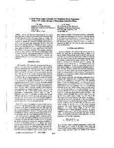
(b) Fig. 3. (a) Output of plant (53) with input (54) (solid line) and output of the dynamic FLS identification model (dash-dotted line). (b) Output of plant (53) with input (54) (solid line) and output of the static FLS identification model (dash-dotted line).

inadequate information is available about the unknown plant and impractical if a large number of inputs is needed [21]. Here, we compare the performance of static and dynamic FLS’s when minimal information is available about the plant. The output of the plant is given by

(53) i.e, it depends on two previous inputs and three previous outputs. Both static FLS’s and feedforward neural networks used in the past to identify systems similar to (53), required and [21] five inputs of the appropriate past values of [i.e.,

206


. This restrictive limitation, which makes such systems hard to use when the order of the plant is unknown, is removed (at least in this example) by using dynamic FLS’s. For our example, we only used and as inputs. The dynamic FLS we used is of the form of (11) with Gaussian membership functions, product inference, , and . We trained our system with a random input uniformly distributed in the interval using the learning algorithm (40)–(52) for 5000 time steps and a learning rate of 0.3. For the testing phase, we used the following inputs:

In our example, we approximated the optimum predictor by (57) (58) We trained the dynamic system (11) as a one-step predictive model of

(59)

(54) We compared the performance of the dynamic FLS with a static FLS that had the same structure, type of membership functions, and inference as the dynamic FLS (11). The only difference between the two systems is the presence of the additional feedback input in the case of the dynamic system. The static FLS was trained using the static backpropagation algorithm given in [15] for 5000 iterations and a learning rate of 0.5. Both systems were identically initialized using the OP method. Fig. 3(a) and (b) shows the output of the plant (solid line) and the outputs of the dynamic and static identification models (dash-dotted lines), respectively. We see that the dynamic FLS has evolved through the dynamic learning algorithm to be able to reproduce the behavior of (53), but the corresponding static system failed to do so. B. Predictive Modeling of a NARMA Process Here, we examine the predictive ability of our dynamic FLS for a nonlinear autoregressive moving average (NARMA) process and compare its performance with static FLS’s of different orders. Static FLS’s essentially belong to the general family of nonlinear autoregressive [NAR(n)] models given by (55) where is an unknown smooth function [2]. Then, assuming that and the error variance is finite, the optimal mean-squared error predictor of , given is the conditional mean, i.e.,

A dynamic FLS belongs to the family of [2] models (56) where, again, is an unknown smooth function, the same assumptions hold for as in the NAR case, and the optimum predictor is

where is a zero-mean uniform white noise process with standard deviation (see Fig. 4). The system had one exogenous input and one feedback input . The FLS was trained for 1500 samples, after 1000 points were allowed for the transients to die out. The model was then tested on the 500 points following the training segment, for 100 Monte Carlo iterations. We similarly trained and tested static FLS’s of different orders [NAR(1)–NAR(6)], with the static backpropagation algorithm in [15]. All FLS’s employed Gaussian membership functions and product inference and contained 50 rules in their rulebase. The results are given in Table I for both dynamic and static FLS’s for different values of . It is obvious that the NARMA(1, 1) dynamic FLS outperforms all static FLS’s. The NAR(1) FLS outperforms all other static systems in both in-sample and out-of-sample performance. The mean-suared error (MSE) for the NAR model increases dramatically when increasing the number of inputs from one to two, but it decreases gradually as the number of inputs continues to inrease. The learning rate was set conservatively to 0.1 for the and cases, and to 0.07 for the case. When starts becoming too large (i.e., , the dynamic system starts to exhibit oscillatory behavior and, finally, becomes unstable. V. CONCLUSION We have presented a formulation for dynamic NSFLS’s, with two main distinguishing features: 1) they generalize static NSFLS’s and 2) they generalize Singleton FLS’s. Extensive comparisons between singleton and non-Singleton FLS’s are given in [13]–[15]. In this paper, through several examples, we have demonstrated that dynamic NSFLS’s can significantly outperform static NSFLS’s in different applications. We have also derived a dynamic learning algorithm to train the system parameters given a sequence of input–output pairs. The dynamic learning algorithm (40)–(52) has characteristics similar to the static backpropagation algorithm for Singleton [23] and non-Singleton [15] FLS’s. It can be initialized based on linguistic information, or using a simple procedure like the one-pass method. This kind of initialization, as opposed to random initialization as in the neural network case, can constrain the search space during optimization, thus resulting in much faster convergence. Since the parameters being updated with the learning algorithm are directly associated with the information in the rule base, the linguistic meaning of the rules is preserved throughout the training process. The learning algorithm for dynamic NSFLS’s also includes training


Fig. 4. Nonlinear autoregressive moving average process (59) with

207

= 0:3.

TABLE I PREDICTIVE MODELING RESULTS FOR THE NARMA(1, 1) PROCESS (59). ALL SYSTEMS WERE TRAINED FOR 1500 SAMPLES, AFTER 1000 POINTS WERE ALLOWED FOR THE TRANSIENTS TO DIE OUT. ALL RESULTS WERE AVERAGED OVER 100 MONTE CARLO ITERATIONS

to include the right amount of input uncertainty. Furthermore, if the feedback input is removed, then (40)–(52) reduce to a static backpropagation algorithm [15]. In Section IV-A, we compared the performance of a dynamic FLS trained with the dynamic learning algorithm with that of a corresponding static FLS trained with static backpropagation. Both systems were trained as identification models for a nonlinear dynamic system whose order was not known. The failure of the static system to successfully identify the unknown plant has demonstrated that using static FLS’s to

model dynamical systems may be unsatisfactory [21]. On the other hand, the dynamic FLS was able to capture the behavior of the plant without being explicitly fed all inputs and outputs, . Viewing dynamic NSFLS’s as belonging to the general family of nonlinear autoregressive moving average models and static NSFLS’s as general nonlinear autoregressive models, we have examined their performance in the predictive modeling of a NARMA process. For time series that possess moving average components, dynamic NSFLS’s have proven to pro-

208


duce models that not only have a lower mean-square error, but also are more parsimonious and have better generalization capabilities.

REFERENCES [1] M. Balazinski, E. Czogala, and T. Sadowski, “Control of metal-cutting process using neural fuzzy controller,” in 2nd IEEE Int. Conf. Fuzzy Syst., San Francisco, CA, Mar. 1993, vol. 1, pp. 161–166. [2] J. T. Connor, R. D. Martin, and L. E. Atlas, “Recurrent neural networks and robust time series prediction,” IEEE Trans. Neural Networks, vol. 5, pp. 240–254, Mar. 1994. [3] D. Dubois and H. Prade, Fuzzy Sets and Systems: Theory and Applications. Orlando, FL: Academic, 1980. [4] , “Fuzzy sets in approximate reasoning—Part 1: Inference with possibility distributions,” Fuzzy Sets Syst., vol. 40, no. 1, pp. 143–202, 1991. [5] Y. Hayashi, J. J. Buckley, and E. Czogala, “Fuzzy neural network with fuzzy signals and weights,” Int. J. Intell. Syst., vol. 8, pp. 527–537, 1993. [6] S. Haykin, Neural Networks: A Comprehensive Foundation. New York: Macmillan, 1994. [7] H. Hellendoorn and C. Thomas, “Defuzzification in fuzzy controllers,” J. Intell. Syst., vol. 1, pp. 109–123, 1993. [8] R. J. Jang and C. Sun, “Neuro-fuzzy modeling and control,” Proc. IEEE, vol. 83, pp. 378–406, Mar. 1995. [9] C. C. Lee, “Fuzzy logic in control systems: fuzzy logic controller—Part I,” IEEE Trans. Syst., Man, Cybern., vol. 20, pp. 404–418, Feb. 1990. , “Fuzzy logic in control systems: fuzzy logic controller—Part [10] II,” IEEE Trans. Syst., Man, Cybern., vol. 20, pp. 419–435, Feb. 1990. [11] J. M. Mendel, “Fuzzy logic systems for engineering: A tutorial,” Proc. IEEE, vol. 83, pp. 345–377, Mar. 1995. [12] , Lessons in Estimation Theory, for Signal Processing, Communications and Control. Englewood Cliffs, NJ: Prentice-Hall, 1995. [13] G. C. Mouzouris and J.M. Mendel, “Non-Singleton fuzzy logic systems,” in 3rd IEEE Proc. Int. Conf. Fuzzy Syst., June 1994, vol. 1, pp. 456–461. [14] , “Non-Singleton fuzzy logic systems: Theory and application,” IEEE Trans. Fuzzy Syst., vol. 5, pp. pp. 56–71, Feb. 1997. [15] , “Nonlinear time series analysis with Non-Singleton fuzzy logic systems,” in IEEE/IAFE Conf. Computati. Intell. Financial Eng., New York, Apr. 1995, pp. 47–56. [16] Y. Muyaram, T. Terano, S. Masui, and N. Akiyama, “Optimizing control of a diesel engine,” in Industrial Applications of Fuzzy Control, M. Sugeno, Ed. Amsterdam, The Netherlands: North-Holland, 1992, pp. 63–71. [17] K. S. Narendra and K. Parthasarathy, “Identification and control of dynamical systems using neural networks,” IEEE Trans. Neural Networks, vol. 1, pp. 4–27, Mar. 1990. [18] O. Nerrand, P. Roussel–Ragot, L. Personnaz, G. Dreyfus, and S. Marcos, “Neural networks and nonlinear adaptive filtering: Unifying concepts and new algorithms,” Neural Computat. vol. 5, no. 2, pp. 165–199, 1993. [19] W. Pedrycz, “Design of fuzzy control algorithms with the aid of fuzzy models,” in Industrial Applications of Fuzzy Control, M. Sugeno, Ed. Amsterdam, The Netherlands: North-Holland, 1992, pp. 139–151. [20] Y. Sakai and K. Ohkusa, “A fuzzy controller in turning process automation,” Industrial Applications of Fuzzy Control, M. Sugeno, Ed. Amsterdam, The Netherlands: North-Holland, 1992, pp. 139–151. [21] P. S. Sastry, G. Santharam, and K. P. Unnikrishnan, “Memory neuron networks for identification and control of dynamical systems,” IEEE Trans. Neural Networks, vol. 5, pp. 306–319, Mar. 1994. [22] H. Tanaka, T. Okuda, and K. Asai, “Fuzzy information and decision in statistical model,” in Advances in Fuzzy Set Theory and Applications, M. M. Gupta, R. K. Ragade, and R. R. Yager, Eds. Amsterdam, The Netherlands: North-Holland, 1979, pp. 303–320.

[23] L. X. Wang and J. M. Mendel, “Back-propagation fuzzy systems as non-linear dynamic system identifiers,” in IEEE Proc. Int. Conf. Fuzzy Syst., San Diego, CA, Mar. 1992, pp. 1409–1418. , “Generating fuzzy rules from numerical data, with applications,” [24] USC-SIPI Rep. 169, 1991; also in IEEE Trans. Syst., Man, Cybern., vol. 22, pp. 1414–1427, Nov. 1992. [25] L. X. Wang, Adaptive Fuzzy Systems and Control. Englewood-Cliffs, NJ: Prentice-Hall, 1994. [26] P. J. Werbos, “Backpropagation through time: What it does and how to do it,” Proc. IEEE, vol. 78, pp. 1550–1560, Oct. 1990. [27] R. J. Williams and J. Peng, “An efficient gradient-based algorithm for on-line training of recurrent network trajectories,” Neural Computat., vol. 2, pp. 490–501, 1990. [28] R. J. Williams and D. Zipser, “A learning algorithm for continually running fully recurrent neural networks,” Neural Computat., vol. 1, no. 2, pp. 270–280, 1989. [29] L. A. Zadeh, “Fuzzy sets,” Inform. Contr., vol. 8, no. 3, pp. 338–353, 1965. [30] , “Outline of a new approach to the analysis of complex systems and decision processes,” IEEE Trans. Syst., Man, Cybern., vol. SMC-3, pp. 28–44, Jan. 1973. [31] H. J. Zimmermann, Fuzzy Set Theory And Its Applications, 2nd ed. Boston, MA: Kluwer, 1991.

George C. Mouzouris was born in Cyprus in 1966. He received the B.S. (with honors) and M.S. degrees from Brown University, Providence, RI, both in 1990, and the Ph.D. degree from the University of Southern California, Los Angeles, in 1996. From 1990 to 1992, he was with the Digital Signal Processing Group of Texas Instruments, Houston, TX, where he dealt with the design and implementation of signal and image processing algorithms on specialized processors. He is currently with the Signal and Image Processing Institute at the University of Southern California, Los Angeles. His research interests include nonlinear dynamic modeling, fuzzy systems, radial basis functions, neural networks, and financial modeling. Dr. Mouzouris is a member of Tau Beta Pi and Sigma Xi.

Jerry M. Mendel (S’59–M’61–SM’72–F’78) received the Ph.D. degree in electrical engineering from the Polytechnic Institute of Brooklyn, Brooklyn, NY, in 1963. Currently he is a Professor of electrical engineering, Director of Special Educational Projects for the School of Engineering, and Associate Director for Education of the Integrated Media Systems Center, all at the University of Southern California, Los Angeles, where he has been since 1974. He has published over 325 technical papers and is the author or editor of seven books. His present research interests include higher order statistics and neural networks applied to array processing and prediction of nonlinear time-series and fuzzy logic applied to prediction of nonlinear time-series, classification problems, and social science problems. Dr. Mendel is a Distinguished Member of the IEEE Control Systems Society. He was President of the IEEE Control Systems Society in 1986. Among his awards are the 1983 Best Transactions Paper Award for a paper in the IEEE TRANSACTIONS ON GEOSCIENCE AND REMOTE SENSING, the 1992 Signal Processing Society Paper Award for a paper in the IEEE TRANSACTIONS ON ACOUSTICS, SPEECH, AND SIGNAL PROCESSING, and a 1984 IEEE Centennial Medal.