Proceedings of IEEE/ASME International Conference on Advanced Intelligent Mechatronics, Kobe, Japan, 20-24 July 2003
Learning Fuzzy Logic Controller for Reactive Robot Behaviours Dongbing Gu, Huosheng Hu, Libor Spacek Department of Computer Science, University of Essex Wivenhoe Park, Colchester CO4 3SQ, UK Email:
[email protected],
[email protected],
[email protected] Abstract: Fuzzy logic plays an important role in the design of reactive robot behaviours. This paper presents a learning approach to the development of a fuzzy logic controller, based on the delayed rewards from the real world. The delayed rewards are apportioned to the individual fuzzy rules by using reinforcement Q-learning. The efficient exploration of a solution space is one of the key issues in the reinforcement learning. A specific genetic algorithm is developed in this paper to trade off the exploration of learning spaces and the exploitation of learned experience. The proposed approach is evaluated on some reactive behaviour of the football-playing robots. Keywords: robot learning, controller, genetic algorithms.
Q-learning,
fuzzy
logic
I. INTRODUCTION Fuzzy Logic Controllers (FLC) has been widely adopted to design reactive robot behaviours [2][8][17]. The main reasons are due to the uncertainty in both sensory information and motor execution. The behaviours designed by FLCs can map real-valued sensory information to realvalued motor commands through fuzzy inference. FLCs are also known as Fuzzy Classifier Systems (FCSs) since they are rule-based and similar to crisp classifier systems in structure [2][19]. Consequent to successful applications of Genetic Algorithms (GAs) for classifier systems [3], the use of GAs or other Evolution Algorithms (EAs) to evolve FLCs has been investigated in many applications [7][10][11][13][19]. In these applications, the parameters of membership functions of fuzzy sets were learned, and so were fuzzy rules, including choosing input variables for fuzzy rules, determining the number of fuzzy sets for input or output variables, etc. However, due to the large search spaces, most complex encoding schemes in robot applications have been implemented in a simulation environment [9][12]. Most evolution scenarios of FLCs falls into two categories: the Michigan approach and the Pitt approach
[4][13]. In the Pitt approach, a FLC or an entire fuzzy set is encoded as an individual. GAs maintain a population of FLCs to evolve by using genetic operators. An optimal or sub-optimal FLC at the end of evolution can be found by choosing the individual that has highest fitness value. On the other hand, the Michigan approach encodes one rule as an individual. GAs maintain a population of rules and a FLC is represented by the entire population [7][13]. Through evolving rules, an optimal or sub-optimal FLC is composed of the rules with higher fitness values. Many researchers called this approach symbolic evolution [10]. Fitness values of GAs always reflect cumulative rewards received by learning algorithms during the whole course of interaction with the environment. They indicate the quality of a sequence of actions, rather than any individual action. To evaluate individual actions, the credit assignment problem exits. In the evolution of crisp classifier systems, the Michigan approach relies on the rule strengths. The bucket brigade algorithm is used to apportion the rewards to individual rules according to their strengths [3]. The classifiers or rules compete with each other through a biding mechanism. In the Pitts approach, the credit assignment is believed to be made implicitly [14]. Poor individual actions have less chance to survive. In the FLCs, the situation of the Michigan approach becomes more complex since the outputs of FLCs depend at each input state on the activated fuzzy rules, not a single rule. Bonarini defined fuzzy state concept to solve the credit assignment problem in FCSs [1][2]. In his research, each fuzzy rule has a strength value, very similar to the crisp classifier systems. In each fuzzy state, multiple rules are activated. The rewards apportioned for each rule depend on the rule's contribution in fuzzy inference to final outputs. The rule's contribution in each fuzzy state is proportional to its activated degree in the state. The rewards can be apportioned to each rule in terms of the action temporal sequence (TD learning) and the rule spatial structure (bucket brigade learning). The Fuzzy Q-learning method proposed in [5][9] has similar ideas to the Michigan approach. There are a fixed
number of rules for a FLC. For each fuzzy rule, a q value is defined for each fuzzy consequence, which is the estimated cumulative reward for the fuzzy antecedents and fuzzy consequence pair of the rule. Q-learning is used to update these q values. Optimal or sub-optimal FLC can be constructed by choosing the fuzzy consequence with the highest q value for each rule. The exploration of state and action spaces in Q-learning or other reinforcement learning can affect both the learning convergence and the learning rate. Taking the greedy actions or exploiting the previous experience too much during the learning would lead to local optima. The learning algorithms would fail to find good actions. On the other hand, taking random actions or exploring the spaces too much would lead to slow learning rates. Thrun classified the exploration strategies into two catalogues: undirected or directed exploration according to whether or not the exploration strategies rely on knowledge about the learning process itself [18]. Both the random walking exploration and the Boltzmann distributed exploration are grouped into the undirected class, which is less efficient. The so-called knowledge about the learning process can be about frequency (how many times the states or actions are being visited so far) or about recency (how recently the states or actions are being visited). Most directed exploration strategies are heuristic based. They have been applied for discrete reinforcement learning only. The attempt to apply the directed exploration for continuous learning has been made in [5][9] where the frequency has been discounted by the activated degree of fuzzy rules. This paper addresses the problem of evolving FLCs. The rule strength is used to evaluate a rule and updated by Q-learning according to the rewards. This will guarantee to apportion the rewards according to the action temporal sequence and the rule spatial structure. A specific GA is used to implement the solution exploration. Genetic operators will select the rules according to fitness values of the entire fuzzy set and the individual fuzzy rule strengths. The rest of the paper is organised as follows. Section II formulises a fuzzy behaviour. Section III illustrates the fuzzy Q-learning that describes how to apportion the rewards to individual fuzzy rules. The experimental results are presented in Section IV. Finally, section VI concludes the paper.
input state variables sI (I=1, …, N) in a state vector S. For each input state variable sI, LI fuzzy sets are defined. We denote the jth fuzzy set of the ith input state variable as
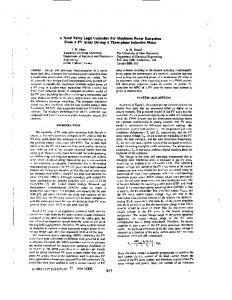
F ji where jI=1… Li. A quadruple of (pa, pb, pc, pd) is employed to represent a triangle or a trapezoid membership function of a fuzzy set as shown in Figure 1 where pb = pc for the triangle shape. The membership degree for a fuzzy set F
A behaviour is a mapping from sensory data or an environment state vector S to a motor action a. It can be expressed as a = B(S) where B is the mapping function. The FLC can be used to implement the function B. Assuming there are N sensory inputs for a behaviour B, i.e. there are N
is expressed as: p d − si pd − pc s − pa 0, i pb − pa
max
µ
F
ji
(s ) = i
0,
max
s s
1
i
> pc
i
< pb
otherwise
M e m b e r sh ip D e g r e e
1 .0
si pa
pb
pc
pd
Figure 1 A membership function of a fuzzy set The total number of fuzzy rules M is the product of the number of fuzzy sets of all input state variables. N
M = ∏ Li i =1
There is only one output variable for each behaviour. There exist K walking commands denoted by ck (k=1,…,K) [6], which can be used for the output. K fuzzy singletons are defined as the fuzzy output. The mth fuzzy rule (m=1,…,M) is denoted as: m
m
F j1 AND … AND sN is F jN k THEN a is cm
Rm: IF s1 is
where II. FUZZY LOGIC CONTROLER
ji
F
jim
(1)
is the jth fuzzy set of the ith input state variable
in the mth rule.
cmk is the kth fuzzy singleton in the mth
rule. The activation value of the mth rule is calculated by Mamdani’s minimum fuzzy implication:
α m ( S ) = min( µ
F
j1m
( s1 ),..., µ
F
m jN
( s N ))
(2)
The crisp output a or the behaviour function stimulated by an input state S after fuzzy reasoning, is calculated by the centre of area method (COA): a = B( S ) =
M
α ( S ) ⋅ c mk m
m =1
M m =1
(3)
α (S ) m
III.FUZZY Q-LEARNING In the Markov decision process frame, the learning robot selects an action at according to its current state St and current experience Q(St, at) values. The action at is executed and the robot moves to next state St+1 with a reward rt from its environment. Then, the learning algorithm is run based on the credit assignment mechanism. In the discrete Qlearning, a look-up table can be built up by listing the stateaction pairs with their Q values. It is impossible to do so in continuous case where the state and action are not discrete. FLCs discussed in the section II can map a state St to an action at. It can also map a state-action pair (St, at) to a Q(St, at) value in the continuous state space [5]. It is very similar to the continuous Q-learning using the connectionist systems [15] where the generalisation of the Q value is implemented by a neural network. The following expression is a rule in a FLC for the mapping. Rm: IF s1 is F
j1m
THEN Q is
where
jNm
AND … AND sN is F
AND a is
cmk
qmk
(4)
qmk is the kth q value in the rule m. Following the
same fuzzy inference in (2), the Q value is calculated as: Q(St , at ) =
M
α m ( S t ) ⋅ q mk
m =1
M
α m (St )
(5)
m =1
Assume that the fuzzy sets are known and the fuzzy sets of the action are fuzzy singletons. Therefore, the Q value error is fully caused by the change of q values. For the onestep Q-learning, the output of (2) is Q(St, at) at time step t. Its estimated value is rt + γ max Q . Then, the error between them is: ∆Q ( S t , a t ) = rt + γ max Q ( S t +1 , a t +1 ) − Q ( S t , a t )
(6)
at +1
By the gradient algorithm, the change of the q value is: ∆q mk = α ⋅ ∆Q ⋅
∂Q ( S t , a t ) ∂q mk
= α ⋅ ∆Q ⋅
α m (St ) M
α m (St )
m =1
(7)
For the multi-step Q-learning, an eligibility trace of the TD learning is maintained for each q value. The replacement trace is defined as:
e( m, k ) =
1
m = mt , k = k t
λγe( m, k )
otherwise
(8)
where mt and kt denote the rule number and action number at the time step t. The updating formula for the q value become : (9) qmk = qmk + q mk ⋅ e(m,k) IV. GA EXPLORATION Reinforcement learning algorithms need a lot of time to find actions that lead to higher rewards if no enough experience is available. Once some experiences are obtained, the algorithms bias their actions on the experience that may not be optimal. A detailed discussion on the exploration strategies is given in [18]. GA is used in this research to explore the solution space. A FLC is encoded as an individual. A population is maintained. A fitness value returned from the environment is assigned to a FLC in the population after each trial. This looks like the Pitts approach. However, we keep two kinds of fitness values for learning algorithms: high-level fitness value for a FLC (or a set of fuzzy rules) and low-level strength for a fuzzy rule. The proposed GA evolves the FLCs based on both of them. Due to the antecedents of a FLC being pre-defined, only the FLC consequences are encoded as chromosomes. There are M rules in one FLC, meaning that there are M fuzzy consequences in one FLC. Therefore, one chromosome has M genes. The first gene corresponds to the first rule’s consequence. Each gene could be one of fuzzy singletons ck as defined in section II and illustrated in Figure 2.
c k1
c k2
……
c kM
Figure 2 An individual encoding The functions used in the GA include: q Initialisation: The first generation is initialised randomly. Each gene in each chromosome is chosen from the K fuzzy singletons evenly. q Elitist: The best individual in current generation is automatically copied into next generation. q Selection: Individuals are copied into next generation as their offspring according to their fitness values. The individuals with higher fitness values have more
q
q
offspring than those with lower fitness values. The roulette wheel selection is used. Crossover: The crossover will happen for two individuals with the crossover probability pc. The idea is to select the genes with higher rule strengths from two parents to produce an offspring. Mutation: The mutation is taken for one gene of an offspring with the mutation probability pm. The operator is to choose one fuzzy singleton from the allowed set to replace the current gene with an adaptive method. The adaptive method relies on the rule strength. The Bolzmann function is used to implement this adaptive process. IV. EXPERIMENTS
its head to track the ball. Simultaneously, sensor process algorithms of the robot find the ball size and its head pan angle. These two variables are employed as inputs of the behavior, as shown in Figure 3. Pan angel (p )
Direction (θ )
Tilt angel (t)
Figure 3 the ball-chasing behaviour
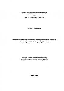
The learning architecture is shown in Figure 4. The environment provides the current state and the The experimental environment consists of a football pitch reinforcement signal to the GA and Q-learning algorithms. used for the Sony legged robots to play football. The Sony The learning algorithms produce the actions to perform in legged robots have some limited vision ability, so they can the environment. There are two parts within a FLC: find a ball and move to it. Additionally, a global CCD activation calculation and action selection. The activation colour camera is mounted on the ceiling to provide global calculation produces the activation degrees of fuzzy rules position information to the proposed learning system. This based on the current environmental state. The action is mainly because the localisation by odometry is not selection produces the actions based on the activation accurate. The global monitor can provide robot and the ball degrees and the current population. The Q-learning position information to the robot via a cable link. algorithm executes the credit assignment to update the rule A simulator is implemented on a PC computer in order strengths based on the reinforcement signal from the to verify the algorithms and reduce the learning time. The environment, the activation degrees, and the current simulator is statistically modelled by measuring real robot environmental state. The GA maintains a population of the motion. The learning system is to provide the reinforcement FLCs and evolves them according to the reinforcement of the environment to the robots to indicate if their goals are signal and the rule strengths. achieved. The behaviour starts when the robot finds a ball. Two methods were adopted in the experiments for both The robot will trigger its vision-tracking algorithm to move simulations and real robots. The first experiment method employed the Pitts approach, which doesn't use the rule strength information and no temporal credit assignment. The second experiment Q-learning GA method employed the approach rule strength proposed in this paper. The population a set of action size was 10, the crossover probability was 0.2, and the mutation probability FLC was 0.1. In simulation experiments, 30 generations were evolved for both Action Activation methods. In real-robot experiments, 20 Selection Calculation activated degree generations were evolved for both methods. reward action The fitness mean values and the state standard deviations are shown in Figure 5 and Figure 6 for both methods. They Environment show that the fitness values are gradually increased and finally Figure 4 The learning architecture converge to a high value. The
dropdowns in the middle of the curve indicates the solution exploration procedures by the mutation and crossover operators. The reduction of the standard deviations reflects the fact that 10 individuals finally tend to have same genes. So their behaviours tend to be same. The difference is that the mean values in Figure 6 increase more quickly than those in Figure 5. Furthermore, the standard deviations tend to decrease more quickly in Figure 6 than in Figure 5. This shows that the proposed method learnt more quickly than the Pitts approach.
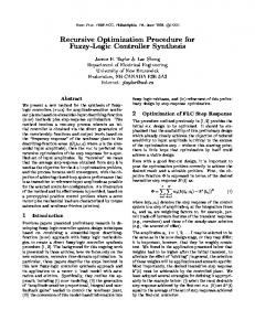
Figure 8 Test in simulation Figure 7 shows the rule strengths of the 7th rule. There are 5 strengths. Only one is activated each time by their competing. Finally, rule q1 won the competition after 300 runs (30 generations). The best FLC was picked up from the last generation to do the test. Figure 8 shows the behavior was successfully evolved. The robot can move to a ball (in the middle of the pitch). Figure 5 Learning of the first method in simulation
Figure 6 Learning of the second method in simulation
Figure 9 Learning of the first method of real robot
Figure 7 Rule strengths
Figure 10 Learning of the second method of real robot
In a real robot, the parameters are same except the generation. The average fitness values and the standard deviations are shown in Figure 9 and Figure 10 for both methods. The same conclusions with the simulation can be drawn from the results. Figure 11 is a test of the behaviour in a real robot with the best FLC in last generation. The behaviour was successfully acquired.
Figure 11 Test of real robot V. CONCLUSIONS AND FUTURE WORK Mapping from the noisy sensory information to imperfect actions to achieve a goal is a challenge in robotics. This paper proposed a solution to the problem. The proposed approach can also be viewed as a Q-learning algorithm with a specific action exploration strategy. The action exploration makes use of the solution search strategies of the GA. The benefits of the "building block" can speed up the learning process. The FLC used acts as a controller and a function approximation of the continuous Q values. In the continuous Q-learning, the neural network is a successful paradigm for the function approximation [17]. Actually FLCs are equivalent to neural networks in function approximation since both of them adopt the distributed structure to approximate a continuous function. The experiment results evaluate the proposed approach. In order to demonstrate its effect on the learning rate, the comparison with pure GA or pure Q-learning will be our next research target. Our future work will also include how to evolve fuzzy antecedents to achieve an automatic design of the mapping. The challenge is that the learning time has to be limited in real robots. REFERENCES [1] Bonarini, A., Comparing Reinforcement Learning Algorithms Applied to Crisp and Fuzzy Learning Classifier
Systems, Proc. of Int. Conf. on Learning Classifier Systems, Morgan Kaufmann, San Francisco, CA, 1999, pp 228-235. [2] Bonarini, A., Evolutionary Learning of Fuzzy Rules: Competition and Co-operation. In W. Pedrycz, editor, Fuzzy Modelling: Paradigms and Practice, Kluwer Academic Press, 1996, pp265-284. [3] Booker, L. B., Goldberg, D. E., Holland, J. H., Classifier System that Learn Their Internal Models, Machine Learning , Vol. 3, 1988, pp161-192. [4] De Jong, K. A., Learning With Genetic Algorithm: An Overview, Machine Learning, VOL. 3, 1988, pp121-138. [5] Glorennec, P. Y. and Jouffe, L., Fuzzy Q-Leering, Proc. of the Sixth IEEE Int. Conf. on Fuzzy Systems, Barcelona, Spain, 1997, pp659-662. [6] Gu, D. and Hu, H., Learning and Evolving of Sony Legged Robots, Proc. Int. Workshop -- Recent Advances in Mobile Robots, Leicester, UK, June 2000. [7] Herrera, F. and Magdalena, L., Genetic Fuzzy Systems: A Tutorial, [8] Hu H. and Gu D., Reactive Behaviours and Agent Architecture for Sony Legged Robots to Play Football, Int. Journal of Industrial Robot, Vol. 28, No. 1, Jan. 2001 [9] Jouffe, L., Fuzzy Inference System Learning by Reinforcement Methods, IEEE Trans. on SMC-PART C, Vol. 28, No. 3, August 1998, pp338-355. [10] Juang, C. F. Lin, J. Y., and Lin, C. T., Genetic Reinforcement Learning through Symbiotic Evolution for Fuzzy Controller Design, IEEE Trans. On SMC-PART B, Vol. 30, No. 2, April 2000, pp290-301. [11] Karr, C. L., Design of an Adaptive Fuzzy Logic Controller Using a Genetic Algorithm, Proc. of the 4th Int. Conf. on Genetic Algorithms, 1991, pp450-456. [12] Lee, S. and Cho, S., Emergent Behaviours of a Fuzzy Sensory-Motor Controller Evolved by Genetic Algorithm, IEEE Trans. on SMC-B, Vol. 31, No., 6, 2001, pp919-929. [13] Michalewicz, Z., Genetic Algorithms + Data Structures = Evolution Programs, Springer, 1995. [14] Moriaty, D. E., Schultz, A. C., and Grefenstette, J, J, Evolutionary Algorithms for Reinforcement Learning, Journal of AI Research, 11(1999), pp241-276. [15] Rummery, G. A., On-Line Q-Learning Using Connectionist Systems, Tech. Rep., CUED/F-INFENG/TR 166, Cambridge University, 1994. [16] Sutton, R. S. and Barto, A.G., Introduction to Reinforcement Learning, MIT Press, 1998. [17] Saffiotti, A., Ruspini, E., and Konolige, K., Using Fuzzy Logic for Mobile Robot Control, Practical Applications of Fuzzy Technologies, H. J. Zimmermann, Editor, Kluwer Academic Publisher, 1999, pp. 185-206. [18] Thrun, S. B. Efficient Exploration In Reinforcement Learning, Tech. Rep. CMU-CS-92-102, 1992. [19] Valenzuela-Rendon, M., The Fuzzy Classifier System: A classifier system for Continuously Varying Variables, Proc. of the 4th Int. Conf. on Genetic Algorithms, Morgan Kaufmann, San Mateo, CA, 1991, pp345-353. [20] Watkins, C. J. and Dayan, P., Technical note: Q-learning, Machine Learning, 8(3/4), 1992, 323-339.