Dynamic Particle Swarm Optimizer for Information Fusion in Non ...

Dynamic Particle Swarm Optimizer for Information Fusion in Non Stationary Sensor Networks Kalyan Veeramachaneni

Lisa Ann Osadciw

Department of EECS Syracuse University Syracuse, NY -13244 [email protected]

Department of EECS Syracuse University Syracuse, NY -13244 [email protected]

Abstract— This paper presents a dynamic particle swarm optimization based search for optimal fusion configuration of sensors in distributed detection network in presence of a nonstationary binary symmetric channel. The wireless channel in sensor networks is a non-stationary random process, which moves the optima of the original problem, otherwise static. The optimal fusion configuration minimizes the probability of error and involves optimal setting of the decision thresholds for the sensors and the optimal fusion rule used at the fusion center. The optimal decision thresholding of a group of sensors in a distributed detection network is a proven intractable problem. Previously a particle swarm optimizer has been used to solve this problem. In this paper a dynamic particle swarm optimizer is used to evolve the optimal decision thresholds of the group of sensors in presence of a non-stationary channel. Performance of the dynamic particle swarm optimizer is compared to the simple particle swarm optimizer in which the particle swarm optimization is restarted after detection of a change. The results demonstrate the effectiveness of the particle swarm in achieving the optima in highly dynamic environments. Dynamic adaptation in the particle swarms towards changes in fitness landscape makes particle swarm optimization an ideal algorithm for multi objective optimization in non-stationary sensor networks.

I.

INTRODUCTION

Our society is currently in a state of information overload with the burgeoning growth of new communication technologies such as WLAN, small inexpensive sensors, and wireless communication technologies. These new sensor networks perform a variety of valuable services including weather warnings, patient health monitoring, building security, air traffic control. As more data and sensors become networked together, the once simple question of “what do we detect and how do we best detect it given the environment and situation at that instant?” is blurred by number of sensors, spectrum, placement, set-up sequence, processing; the list is endless. Process refinement or sensor management can be described as a process that provides automatic and semi automatic control of the group of sensors to achieve the

objectives. The objective of these sensor networks is to maximize probability of detection while minimizing time, power usage and probability of false alarms. The controls for the sensors include, transmitting power, sensor location, detection thresholds and several others. The controls for the network include the set up sequence, the routing used, the communication protocol and several others. Let

{c1 , c2 .........cn } be the ‘n’ controls of the sensors and the i

network that can be changed to achieve required performance. Let {P1 , P2 .............. Pp } be the ‘p’ performance measures, which we need to optimize. Each of the performance measures is a function of the settings at which the network and the sensors are

{

Px = f {c1,c2.........cn} ,{c1,c2.........cn} .......,{c1,c2.........cn} 1

2

}

n

(1)

The problem of optimizing the network configuration in presence of multiple performance measures which are conflicting, or in other words multiple objectives is p ⎛ P desired − Pi achieved ⎞ E = ∑ wi × ⎜ i ⎟ P desired i i =1 ⎝ ⎠

(2)

assuming minimization of E, where n

∑w i =1

i

=1

(3)

Configuration of a sensor network for achieving the above objectives is an intractable problem considering the number of sensors, number of parameters one has to control to achieve those. We have successfully applied particle swarm optimization algorithms to dynamically configure sensor networks to optimize accuracy, time [1 - 4]. Specifically, we defined the optimal configuration of sensor network as a multi objective optimization problem and used particle swarm optimization to search for global optimum.

{

Px = f t,{c1,c2.........cn} ,{c1,c2.........cn} .......,{c1,c2.........cn} 1

2

}

n

(4)

The affect of all these changes result in movement of the optima or appearances of new optima in the fitness landscape. In this paper we show that the swarm algorithms are inherently capable of tracking the changing optima and achieve the optima even when the process is non-stationary during its run time. In other words, with changes occurring in the global optima’s location in the search space the swarm learns and moves in the search space without the need of resetting the swarm. Many researchers have investigated this property of swarm and concluded that the swarm does not get stuck if the optima position is changed. In this paper we exploit this property of swarm to use it for optimization in sensor networks. Also we show that retaining the particle positions even after the optima is shifted helps swarm attain a better minima. We compare the dynamic particle swarm optimizer to a standard particle swarm optimizer, which is started when the change is detected. In this paper a simple problem in wireless sensor networks is chosen to demonstrate the efficacy of swarms in dynamic environments. A distributed detection sensor network (DDSN) is considered. These sensors detect the presence or absence of phenomena and transmit their decisions to a fusion center wirelessly, which fuses all the incoming decisions and accepts or rejects the hypothesis. Once the decision regarding the presence or absence of the phenomena is given by the fusion center the response plans are generated to combat the situation. Detection performance is the primary goal of these types of sensor networks, used in applications such as remote monitoring systems for nuclear power plants, health-monitoring systems for patients. Apart from detection performance of the system, other critical objectives are time and energy. In this paper we present a distributed detection network with a primary aim of maximizing probability of detection and minimizing the probability of false alarms. These are among the different performance measures we optimize for sensor network. In the next section the distributed detection network and the sensor controls, which are varied, and their impact on the performance measures are explained. Also the affect of changing conditions is explained. The particle swarm optimization algorithm and various models that are used to track the moving optima are detailed. Section III describes the formulation of the distributed detection problem. Section IV describes the design of particle swarm optimization

algorithm for the problem. Results are presented in section V. Finally conclusions and future work is presented in Section VI. II.

MOTIVATION

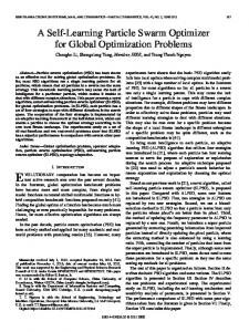
A. The Time Varying Distributed Detection Networks Uncertainty minimization in decision-making has lead to an interesting area called information fusion. This has lead to use of multiple sensors to increase the detection performance. The central idea behind using multiple uncorrelated sensors is that probability that all of them make errors at the same time is extremely low. Decisions from multiple sensors are fused at the fusion center to arrive at a final decision as shown in Figure 2. Ad hoc approaches were originally employed to fuse these decisions from multiple sensors. The simplest approach of all is a majorityvoting rule, which made the decision in the favor of the majority of the sensors. Considering the number of combinations in which the decisions can arrive at the fusion center, the number of ways that they can be combined also increased exponentially. Also, these are heterogeneous sensors and have varying levels of accuracy depending upon overlap between the conditional probability distributions under the two hypotheses. This overlap is based on the thermal noise that it generates during its processing, its received signal power, its location and several other factors. Due to these inherent limitations the sensors make errors and hence lead to incorrect decisions. Thresholding a sensor measurement at a very low value leads to a very high probability of detection, but leads to a high false alarm probability as can be seen by the area under the distribution of Ho above the threshold value. -3

3.5

sens or 1

x 10

3

Likelihood Probability

However, in highly dynamic systems such as sensor networks, a more robust algorithm responding to changes in the environment needs to be designed. Sensor networks are characterized by changing environment conditions affecting the channel through which these sensors communicate, changing processing queues at the processing nodes, changing scenarios. For example, for a group of sensors tracking targets, the number of targets changes from time to time. The performance evaluation functions now change in time and are function of time.

2.5

2

1.5

H1

H0

1

0.5

0 -100

-50

0

50

100 score

150

200

250

300

Figure 1: Sensor Model for Distributed Detection Network Thresholding the sensor measurement above which the hypothesis is accepted needs to be done, such that the probability of detection is maximized while probability of false alarm is minimized. However, both the objectives are highly impossible to achieve simultaneously and is a classic multi objective optimization problem. When more than two sensors are involved in fusion, however, both the errors can be reduced by using a careful optimization scheme. The

reader is referred to [1-5] for theoretical analysis. When multiple sensor decisions are fused, individual thresholding of these sensors as well as the best way to combine their decisions so that both the objectives are optimized is a NP hard problem [11]. In detection theory literature this problem is called optimal decision fusion scheme [1 –4]. For a mathematical explanation of the problem the reader is referred to [1-4, 9]. The problem is defined as setting up of optimal thresholds for participating sensors and the fusion rule to achieve minimum probability of error. A particle swarm optimization based algorithm has been developed to arrive at the optimal decision fusion strategy in [1 - 3]. Sensor 2

Sensor N

Sensor 1

u2

u1

un

C2

C1

y1

Cn

y2 Fusion Center

yn

U0

Figure 2: Distributed Detection Sensor Network Adding another level of complexity to the problem is the wireless channel through which the sensors transmit decisions. The decisions transmitted wirelessly are corrupted by the wireless channel and also affects the detection performance. The strength of the optimal decision fusion strategy generated without consideration of channel is reduced significantly due to presence non-ideal channels [6]. A direct consequence of this is to revise the decision thresholds and the fusion rule based on the channel conditions to achieve optimality [6]. Revising the thresholds, fusion rule compensates for the channel impairments [6]. Intuitively this makes sense, as a fusion strategy can be evolved to neglect the decisions from the sensors with nonideal channels and/ or increasing the threshold for the sensor with an ideal channel between it and the fusion center. The problem of arriving at the optimal fusion strategy, however, still remains intractable. The channel is characterized by the first order moments of the probability of error. However, the channel is a non-stationary random process, and hence these moments change over time. This makes the original intractable problem dynamic with optima in the fitness landscape changing from time to time. B. Particle Swarm Optimization in Dynamic Environments The particle swarm optimization algorithm, originally introduced in terms of social and cognitive behavior by Kennedy and Eberhart in 1995 [4], has come to be widely used as a problem solving method in engineering and computer science. PSO has since proven to be a powerful com-

petitor to genetic algorithms [4]. The technique is fairly simple and comprehensible as it derives its simulation form social behavior of individuals. The individuals, called particles henceforth, are flown through the multidimensional search space, with each particle representing a possible solution to the multidimensional problem. The movement of the particles is influenced by two factors: as a result of the first factor, each particle stores in its memory the best position visited by it so far, called pbest and experiences a pull towards this position as it traverses through the search space. As a result of the second factor, the particle interacts with all the neighbors and stores in its memory the best position visited by any particle in the search space and experiences a pull towards this position, called gbest. The first and the second factors are called cognitive and social components respectively. After each iteration the pbest and gbest are updated if a more dominating solution (in terms of fitness) is found, by the particle and by the population respectively. This process is continued iteratively until either the desired result is achieved or the computational power is exhausted. The PSO formulae define each particle in the D-dimensional space as X i = ( xi1 , xi 2 ,...., xiD ) where the subscript i represents the particle number and the second subscript is the dimension. The memory of the previous best position is represented as Pi = ( pi1 , pi 2 ,...., piD ) and a velocity along each dimension as Vi = ( vi1 , vi 2 ,...., viD ) . After each iteration, the velocity term is updated and the particle is pulled in the direction of its own best position, Pi and the global best position, Pg, found so far. This is apparent in the velocity update equation, [5]. Vid

( t +1)

= ω × Vid

(t )

+ rand (1) ×ψ 1 × ( pid − xid ) + rand (1) ×ψ 2 × ( p gd − xid ) (t )

(t )

(5) (t ) ( t +1) (6) X id = X id + Vid Recently there has been a lot of research in the behavior of particle swarms in dynamic environments. Particle swarms capability to track dynamic optima is detailed in [11 –15]. For dynamically changing systems there are two important things, which need to be done. First detecting that a change has occurred and then designing a response to the change [16]. For a system that has changed, the particles memories which store the best position visited by it so far has no longer the fitness which will match the fitness it possessed before the change. This leads the particles towards a direction where fitness decreases. It should be noted that very simple changes in the algorithm can lead to a detection as well as response to the change in the system. Carlisle et. al [13] suggested resetting the “pbest” vector at regular intervals. In a way this suggests that the memories are removed from time to time while the particle positions, which they reached by learning their memories, are retained. Synchronization of the resetting and the changes in the ( t +1)

system has to be done carefully. Often the dynamics of the system, which changes, is not known. To overcome they also suggested that the resetting could be done whenever there is a change detected in the system. However, this would lead to evaluating the ‘pbest’ vector in every iteration to detect if there is any change. In [17] Carlisle et. al suggested using a sentry particle for every iteration to detect any change in the fitness. In [16] the detection of the change was done by evaluating the ‘gbest’. In [17] Carlisle suggested that re-evaluation of the ‘pbest’ vector whenever the change is detected and then updating the ‘pbest’ with the ‘present’, if a better fitness has been found. By this method the valuable experiences are preserved. In this paper this methodology is adopted. We call this dynamic PSO (DPSO). In this paper a time varying channel is added to our original problem and a dynamic particle swarm optimization algorithm is used to track the moving optima. The change detection phase is not necessary as the changes in channel are detected from time to time by a different routine. However, in other problems in sensor networks that we are dealing with [1, 2], this detection is necessary and we use a sentry particle to detect the changes. Comparisons are done with a methodology in which the particle swarm optimization algorithm is restarted everytime a change is detected. An argument can be made about the quality of the dynamic algorithm by comparing it with simple PSO technique in which the particle swarm is completely restarted when a change is detected.

heterogeneous and are not identically distributed. An assumption of Gaussian noise at the sensor is made. Hence a sensor ‘i’ is characterized by the distribution of the noise and the received signal power level given by the pair (7)

Pi is the recieved power of ith sensor, and

N i (μ , σ ) is an Gaussian noise with mean μ and 2

standard deviation for the sensor are

H 0 : Ni H1 : Pi + N i

σ

th

at the i sensor. The two hypotheses (absence of signal)

(8)

(presence of signal)

(9)

A binary symmetric channel is characterized by

α10i is the probability that transmission of 1 will be i corrupted to zero, α 01 is the probability that transmission of where,

zero will be corrupted to 1. Figure 3. shows a binary symmetric channel 1 − α 10

1

1

α 10 α 01

0

1 − α 01

0

Figure 3: A Binary Symmetric Channel The two types of errors commonly known as probability of false alarms and probability of miss are PFA = P(U 0 = 1/ H 0 ) (11)

PM = P(U 0 = 0 / H1 )

(12)

These errors occur when the final decision after fusion does not match with the true hypothesis. Also, probability of detection is given by PD = 1 − PM (13) Where U 0 is the decision of the fusion center, which takes

on the fusion rule.

Figure 2. shows a sensor network employed for distributed detection. The sensors make decisions and communicate with the fusion center. The channel, characterized by a binary symmetric channel in this paper, corrupts the decisions from the sensors. Each sensor in the network is characterized by a model, which is defined by its conditional distributions under the two hypotheses H 0 , H1 as shown in Figure 1. The sensors are

where,

(10)

in the decisions from the local sensors and fuses them, based

III. PROBLEM FORMULATION FOR DISTRIBUTED DETECTION IN PRESENCE OF NON IDEAL CHANNELS

si = {Pi , N i (μ , σ 2 )}

β i = {α10i , α 01i }

The minimization function for a distributed detection network is given by E = CFA × PFA + CM × PM (14) Where, PFA is probability of false alarm, PM is probability of miss, CFA is cost of false alarm, CM is cost of a miss. CFA = 1 − CM (15) Probability of false alarm and probability of miss are functions of PFA = g1(s1, s2 ,........., sn , λ1, λ2..........λn , f , β1, β2 ,....., βn ) (16) Similarly,

PM = g2 (s1, s2 ,........., sn , λ1, λ2..........λn , f , β1, β2 ,....., βn ) (17) where, {s1, s2 ,........., sn} are the sensor models expressed by

conditional probability distributions, {λ1, λ2..........λn} are the thresholds for the N sensors. {β1, β2 ,....., βn} , are the binary symmetric channel conditions between the ith sensor and the fusion center respectively. f is the fusion rule used to fuse the incoming decisions. Under changing channel conditions equations (16) and (17) become

PFA() t =g1(s1,s2,.........,sn,λλ t β2(),....., t βn()) t 1, 2..........λn, f,β1(),

(18)

PM() t =g2(s1,s2,.........,sn,λλ t β2(),....., t βn()) t 1, 2..........λn, f,β1(),

(19)

Hence equation (14) becomes

E (t ) = CFA × PFA (t ) + CM × PM (t )

(20)

For detail about formulation of PFA and PM the reader is referred to [1- 6]. Equation (20) is of the form (2) with two performance parameters PFA, PM IV.

PARTICLE SWARM OPTIMIZATION FOR A DDSN

Each particle in this problem has ‘N+1’ dimensions, where N is the number of sensors in the sensor network. Each of the N dimensions is a threshold at which a particular a sensor is set. The ‘N+1’ th dimension is the fusion rule, which determines how all the decisions from the sensors are fused. Hence the representation of each particle is, X i = ( λi1 , λi 2 ..........λin , f i ) (8) The sensor thresholds are continuous. The fusion rule, however, is a binary number having a length of log2 p

p = 2 2 for ‘N’ sensors, with a real value varying from 0 ≤ Re( f ) ≤ p − 1 . For binary search N

bits, where

spaces, the binary decision model as described in [5] is being used. Hence the PSO used in the paper is a hybrid of both binary PSO and continuous PSO; binary for evolving the fusion rule, continuous for thresholds. The two objectives for this problem are given by (16) and (17). The goal is to minimize E. At each iteration the particles representing the solution for the problem are evaluated for these objectives using the weighted cost function (20). The memory of the particles is updated if it finds better minima. The particles are moved in the search space based on equations (5) and (6) and these steps are iteratively repeated till convergence occurs or the requirements are fulfilled. Changes in the channel conditions are detected and the ‘pbest’ vector is updated once a change is detected. In the following section the results achieved by applying the particle swarm optimization problem with minor modifications for adapting to dynamically changing environment are presented. V.

RESULTS AND DISCUSSION

A. Experimental Settings The experiments were conducted by changing the channel conditions during the single run of PSO. A 5-sensor test bed is used to test the performance of the swarm under changing channel conditions. The sensor models used in [1] are used in this paper. 10 particles with equal weight for social and cognitive component were used for evolution. We ran the experiments for 2000 iterations in all the experiments. Three experiments were conducted with varying degree of channel volatility. The change in channel is achieved by changing {β1, β2 ,....., β5} where each

β i = {α10i , α 01i } . In

the first, the channel was changed 4 times during the

simulation moving the optima four times. The times when the channel was varied were {300, 600, 1200, and 1800}. In the second experiment the frequency of change of channel was increased. The times of change of channel in this experiment were {100, 400, 700, 1000, 1300, 1600, and 1900}. In the third experiment, the channel was changed after every 50 iterations. In the third experiment the values

α10i , α 01i are chosen randomly from the set ⎧0.1, 0.01, 0.001, 0.0005, 0.0009, 0.000008, 0.4,⎫ ⎨ ⎬ ⎩ 0.8, 0.008, 0.08 ⎭

of

with equal probability. It should be noted that the set has been carefully designed in order to have a chaotic behavior of the optima. For all the three experiments we conducted a parallel experiment by running the standard PSO (SPSO) algorithm with the final channel conditions that were detected during the last change in the channel. For example the channel condition for the first experiment is {β1(t1), β2 (t1),....., β5 (t1)} , where t1 = 1800. Similarly for second experiment {β1(t2 ), β2 (t2 ),....., β5 (t2 )} , where t2 = 1900. For third experiment the final channel condition was {β1(t3 ), β2 (t3 ),....., β5 (t3 )}, where t3 = 1950. A comparison is made between the solutions achieved at the end of ‘n’ iterations, where ‘n’ is equal to 2000-ti for all the three cases. B. Results and Analysis Figure 4, 5, 6 show the dynamic PSO’s (DPSO) behavior to changing optima. It can be seen that PSO is able to track the changing minima location in the search space. Evaluations of particle swarms ability to track optima have been done using a distance from optima approach in [12 –17]. However, in real applications this information is not available and hence alternate methodologies to evaluate particle swarms behavior in dynamic environments should be established. In this paper we compare it with the approach in which we restart the particle swarm when a change is detected. Hence, if a system changes ‘n’ times during the run of a dynamic particle swarm, we note the ‘nth’ change and run a standard particle swarm optimizer. The quality of solutions achieved against the number of iterations by this particle swarm is compared to the particle swarm tracking the optima. Intuitively, this makes sense, as we want to determine if it is beneficial to start the swarm all over again when there is a change detected in the landscape. In other words is it beneficial in terms of fitness evaluations to retain the current positions in the fitness landscape and responding to the changes by resetting the memory.

Table 1: DPSO vs. SPSO for the same number of iterations

Figure 4: Probability of Error vs. Iterations of PSO for a single trial; Experiment 1

Experiment No.

Probability of Error- DPSO

Probability of Error SPSO

1.

0.0072

0.0460

2.

0.0230

0.0479

3.

0.1718

0.0280

In Table 1 results averaged over 12 trials are given. As can be seen that the probability of error achieved by the DPSO which is tracking the changing optima is lower than the minima achieved by the restarting the PSO. This emphasizes that the particle swarms tracking the optima in dynamic environments are located at significant positions in the search space and it is beneficial to retain those positions and adapt to the changing landscape. The strategy where the particle swarm optimization was restarted (SPSO) after a change has been detected performed significantly poorer. In the third experiment however, where the optima was changed chaotically, the restarting of the swarm attained better performance. It should be noted, however that the DPSO had only 50 iterations after the change. On the contrary by restarting the swarm a better minima was found within the same 50 iterations. It can be expected that the DPSO will outperform if the number of iterations are increased as the swarm in these few iterations is recovering from the change in the optima location.


The results also show particle swarms ability to achieve minima in dynamic environments. This is a significant property enabling particle swarm to be applied to real time optimization problems such as optimal configuration of sensor networks. VI.


CONCLUSIONS AND FUTURE WORK

In this paper the efficacy of particle swarms in tracking optima in a non-stationary sensor networks is demonstrated. A simple optimization problem in sensor networks, i.e., minimizing the probability of error was chosen to demonstrate this. Results achieved show the ability of PSO to track the optima and achieve the optima quickly even after a change. This has been illustrated by observing the difference in optima achieved by the dynamic tracking PSO and restarting the swarm after the change. The results show that the dynamic PSO perform significantly better than the strategy in which the search is restarted after the change is detected. In future new versions of PSO will be modeled to increase its ability to track changing optima. Particle swarm optimization is being used to solve other dynamic problems in sensor networks.

References

[8]

[1]

[9]

[2]

[3]

[4]

[5]

[6]

[7]

Kalyan Veeramachaneni, Lisa Osadciw, “ Dynamic Sensor Management Using Multi Objective Particle Swarm Optimizer”, SPIE Defence and Security Symposium, April 16-20, 2004, Orlando, Florida. Lisa Osadciw, Kalyan Veeramachaneni, “Multi Objective Optimization Using Particle Swarms for Sensor Management”, IEEE Upstate Kalyan Veeramachaneni, Lisa Osadciw, Pramod Varshney, “Adaptive Multimodal Biometric Fusion Using Particle Swarm Optimizer”, SPIE Defence and Security Sympoisum, April 12-20, 2003, Orlando, Florida. Kalyan Veeramachaneni, Lisa Osadciw, Pramod Varhsney, “Adaptive Multimodal Biometric Management Algorithm”, IEEE Transactions on Systems, Man and Cybernatics, Vol. 35, No. 4, August, 2005. Kalyan Veeramachaneni, Yan Weizhong, Kai Goebel, Lisa Osadciw, “Improving Classifier Fusion Using Particle Swarm Optimization”, Submitted to International Information Fusion Conference, July, 2006, Florence Italy. Biao Chen, Peter K. Willet, “On Optimality of the Likelihood-Ratio Test for Local Sensor Decision Rules in the Presence of Nonideal Channels”, IEEE Transactions on Information Theory, Vol. 51, No.2. February, 2005. Kalyan Veeramachaneni, Thanmaya Peram, Lisa Ann Osadciw, Chilukuri Mohan, “Optimization Using Particle Swarms with Near Neighbor Interactions”, GECCO, 2003, July, 2003.

[10]

[11]

[12] [13]

[14] [15]

[16]

[17]

James Kennedy, Russell Eberhart and Shi, Y.H., Swarm Intelligence, Morgan Kaufman Publishers, 2001. Pramod K. Varshney, Distributed Detection and Data Fusion, Springer-Verlag, New York Inc., 1996. Randy Cogill, Sanjay Lall, “Decentralized Stochastic Decision Problems and Polynomial Optimization”, Proceedings of the 2004 Annual Allerton Conference on Communication, Control, and Computing. J. N. Tsitsiklis and M. Athans, “On Complexity of decentralized decision making and detection problems”, IEEE Transactions on Automatic Control, vol. AC-30, pp., 440-446, 1985. Xiaodong Li, Khanh Hoa Dam, “Comparing Particle Swarms for Tracking Extrema in Dynamic Environments”, Anthony Carlisle, Gerry Dozier, “Adapting Particle Swarm Optimization to Dynamic Environments”, In proceedings of International Conference on Artificial Intelligence, Las Vegas, Nevada, USA, 2000. Daniel Parrott, Xiaodong Li, “A Particle Swarm Model for Tracking Multiple Peaks in a Dynamic Environment using Speciation”, Eberhart R. C., and Shi Y, “ Tracking and Optimizing Dynamic Systems with Particle Swarms”, Proceedings of the 2001 Congress on Evolutionary Computation, CEC 2001. Hu X, Eberhart R. C., “Adapting Particle Swarm Optimization: Detection and Response to Dynamic Systems”, Proceedings of IEEE Congress on Evolutionary Computation, CEC, 2002. Carlisle, A., Dozier, G., “Tracking Changing Extrema with Adaptive Particle Swarm Optimizer”, ISSCI, 2002 World Automation Congress, Orlando, FL, USA, June 2002.