Inertia-Adaptive Particle Swarm Optimizer for Improved Global Search Kaushik Suresh, Sayan Ghosh, Debarati Kundu, Abhirup Sen, Swagatam Das and * Ajith Abraham 1
Department of Electronics and Telecommunication Engineering Jadavpur University, Kolkata, India * Center of Excellence for Quantifiable Quality of Service, Norwegian University of Science and Technology, Trondheim, Norway
[email protected]
Abstract This paper describes a method for improving the final accuracy and the convergence speed of Particle Swarm Optimization (PSO) by adapting its inertia factor in the velocity updating equation and also by adding a new coefficient to the position updating equation. These modifications do not impose any serious requirements on the basic algorithm in terms of the number of Function Evaluations (FEs). The new algorithm has been shown to be statistically significantly better than four recent variants of PSO on an eight-function test-suite for the following performance matrices: Quality of the final solution, time to find out the solution, frequency of hitting the optima, and scalability.
1. Introduction The concept of particle swarms, although initially introduced for simulating human social behavior, has become very popular these days as an efficient means of intelligent search and optimization. The Particle Swarm Optimization (PSO) [1, 2], does not require any gradient information of the function to be optimized, uses only primitive mathematical operators and is conceptually very simple. PSO emulates the swarming behavior of insects, animals herding, birds flocking and fish schooling, where these swarms forage for food in a collaborative manner. PSO also draws inspiration from the boid’s method of Craig Reynolds and socio-cognition [2]. Particles are conceptual entities, which search through a multidimensional search space. At any particular instant, each particle has a position and velocity. The position vector of a particle with respect to the origin of the search space represents a trial solution to the search problem. PSO is however not free from false and/or premature convergence, especially over multimodal fitness landscapes. In this article, we describe a new variant of the basic PSO, which improves the
performance of the algorithm in two ways. Firstly, the inertia factor of the classical PSO has been adapted in such a fashion that whenever a particle moves far away from the globally best position found so far by the swarm, the effect of its inertial velocity will be minimal. Secondly, a momentum factor has been added to the position updating equation of the classical PSO, which gives greater mobility to the particles even when their velocities become very low due to false convergence to some local minima.
2. The Particle Swarm Optimizers 2.1 The Classical PSO PSO is in principle, a multi-agent parallel search technique and bears many common features with other population based optimization techniques, such as the Genetic Algorithms (GAs) [3]. PSO starts with the random initialization of a population of candidate solutions (particles) over the fitness landscape. However, unlike other evolutionary computing techniques, PSO uses no direct recombination of genetic material between individuals during the search. Rather it works depending on the social behavior of the particles in the swarm. Therefore, it finds the global best solution by simply adjusting the trajectory of each individual towards its own best position and toward the best particle of the entire swarm at each time-step (generation). In a D-dimensional search space, the position vector of the i-th particle is given by r X i = ( xi ,1 , xi ,2 ,......., x i , D ) and velocity of the i-th r particle is given by Vi = (v i ,1 , v i ,2 ,......., v i , D ) .
Positions and velocities are adjusted and the objective r function to be optimized f ( X i ) is evaluated with the new coordinates at each time-step. The velocity and position update equations for the d-th dimension of the i-th particle in the swarm may be represented as:
vi ,d (t ) = vi ,d (t − 1) + C1 * rand1 * ( pbesti ,d − xi ,d (t − 1)) + C2 * rand 2 * ( gbestd − xi ,d (t − 1)) x i ,d (t ) = x i ,d (t − 1) + v i ,d (t )
that
pbesti ,d − xi , d and
enough, (1)
where rand1 and rand 2 are random positive numbers uniformly distributed in (0,1) and are drawn anew for each dimension of each particle. pbest is the personal best solution found so far by an individual particle while gbest represents the fittest particle found so far by the entire community. The first term in the velocity updating formula is referred to as the ‘cognitive part’. The last term of the same formula is interpreted as the ‘social part’, which represents how an individual particle is influenced by the other members of its society. C1 and C2 are called acceleration coefficients and they determine the relative influences of the cognitive and social parts on the velocity of the particle. The particle’s velocity is clamped to a r maximum value Vmax = [v max,1 , v max, 2 ,..., v max, D ]T . If in d-th dimension, vi ,d exceeds v max, d specified by the user, then the velocity of that dimension is assigned to sign(v i , d ) * v max, d , where sign(x) is the triple-valued signum function.
2.2 Some significant variants of the classical PSO Since its introduction by Kennedy and Eberhart in 1995, PSO has been subjected to empirical [4-6] and theoretical [7,8] investigations by several researchers. Shi and Eberhart [9] introduced a new parameter ω , now well-known as inertia weight, to the original version of PSO in the following way: vi,d (t ) = ω.vi,d (t −1) + C1 * rand1 * ( pbesti,d − xi,d (t − 1))
+ C2 * rand2 * ( gbestd − xi,d (t − 1)) (2) The inertia weight is used to balance the global and local search abilities. A large inertia weight is more appropriate for global search and a small inertia weight facilitates local search. Some other significant variants of the classical PSO can be traced in [9 – 14].
3. The Inertia-adaptive PSO Algorithm Premature convergence occurs when the positions of the most of the particles of the swarm stop changing over successive iterations although the global optimum remains undiscovered. This may happen if the swarm uses a small inertia weight [15] or a constriction coefficient [7]. From the basic equations of PSO, we see that if vi ,d is small and in addition to
gbest d − xi ,d
are small
vi ,d cannot attain a large value in the
upcoming generations. That would mean a loss of exploration power. This can occur even at an early stage of the search process, when the particle itself is the global best causing pbest i ,d − x i ,d and
gbest d − xi ,d to be zero and, gets damped quickly with the ratio ω . Also the swarm suffers from loss of diversity in later generations if pbest and gbest are close enough [17]. In this work we incorporate two modifications into the classical PSO scheme which prevent false convergence and helps provide excellent quality of final result without imposing any serious burden in terms of excess number of function evaluations (FEs). The first of these modifications involves modulation of the inertia factor ω according to distance of the particles of a particular generation from the global best. The value of ω for each particle is given by: dist i , ω = ω 0 .1 − (3) max_ dist where ω 0 = rand (0.5,1) , disti is the current Euclidean distance of i-th particle from the global best i. e. 1
D 2 dist i = ( gbest d − x i ,d ) 2 (4) d =1 and max_dist is the maximum distance of a particle from the global best in that generation i.e. (5) max_ dist = arg max(disti )
∑
i
This modulation of the inertia factor ensures that in case of particles that have moved away from the global best, the effect of attraction towards global best will predominate. To avoid premature convergence this we must ensure that the particle has mobility in the later stages. In order to achieve our purpose, the position update equation is modified as follows: xi ,d (t ) = (1 − ρ ).xi ,d (t − 1) + vi ,d (t ) (6) where ρ is a uniformly distributed random number in the range (-0.25, 0.25). From now on, we shall refer to this new algorithm as IAPSO (Inertia-adaptive PSO).
4. Experimental Results 4.1 Benchmark functions We have used eight well-known benchmarks [14] to evaluate the performance of the proposed algorithm. Here the proposed algorithm has been compared with the classical PSO algorithm and four of its significant variants over these benchmark functions. In Table 1, D
represents the number of dimensions (we used D = 30 and 60). An asymmetrical initialization procedure has been used here following the work reported in [6]. 4.2 Algorithms compared
Simulations were carried out to obtain a comparative performance analysis of the proposed IAPSO algorithm with respect to: (a) the basic PSO (BPSO) with constant inertia weight (b) PSO-TVIW [5] (c) HPSO-TVAC [11] (d) MPSO-TVAC [11], and (e) CLPSO [12]. 4.3 Population Size
Shi and Eberhart [15] showed that population size had hardly any effect on the performance of PSO. van den Bergh and Engelbrecht [19] also reported that though there is slight improvement in solution quality with increasing swarm sizes, a large swarm increases the number of function evaluations (FEs) required to converge to a prescribed error limit. In this work, for all algorithms over all problems, we kept a constant population size of 40 particles 4.4 Simulation Strategy
To make the comparison fair, the populations for all the competitor algorithms (for all problems tested) were initialized using the same random seeds. We have run two separate sets of experiments over the eight benchmark functions. To judge the accuracy of different PSO-variants, we first let each of them run for a very long time over every benchmark function, until the number of function evaluations (FEs) exceed a given upper limit (which was fixed at 106). We then record the final best fitness achieved by each algorithm. In the second set of experiments we run the PSO-variants on a function and stop as soon as the best fitness value determined by the algorithm reaches below a predefined threshold value (here 10-3 for all benchmarks). Then we note the number of FEs the algorithm takes. A lower number of FEs corresponds to a faster algorithm. We employed the best set of parameters for all competitive algorithms, as found in the relevant literatures. For IAPSO, we took C1 = C 2 = 2.00 . All the algorithms discussed here have been developed from scratch in Visual C++ on a Pentium IV, 2.3 GHz PC, with 1024 KB cache and 2 GB of main memory in Windows XP environment.
Table 1. Benchmark functions used Function Sphere function
Mathematical Representation D r f1 ( X ) = xi2
Rosenbrock’s function
r D−1 f2 (X ) = [100( xi +1 − xi2 ) 2 + ( xi − 1) 2 ]
Rastrigin’s function
∑ i =1
∑ i =1
r f3 ( X ) =
D
∑ (x
2 i
− 10 cos(2πxi ) + 10)
i =1
Griewank’s function
r f4 (X ) =
D
xi +1 i
D
xi2
∑ 4000 − ∏cos i =1
i =1
n r 1 f5( X ) = −20exp − 0.2 xi2 − D i =1 1 n exp cos(2πxi ) + 20+ e D i=1
∑
Ackley’s function
∑
r f6 ( X ) = Weierstrass function
k max k [ a cos( 2πb k ( xi + 0 .5))] i =1 k = 0 D
∑ ∑
k max
−D
∑ [a
k
cos( 2πb k ⋅ 0.5)]
k =0
a = 0 .5,
b = 3,
k max = 20
D−1 r π f7 (X) = {10sin2 (πyi +1) + (yi −1)2 D i =1
∑
Generalized Penalized function 1
D
.[1+10sin2 (πyi +1)]+ ( yn −1)2}+
∑u(x ,10,100,4) i
i =1
D−1 r f8 ( X ) = 0.1{sin2 (3πx1) + (xi − 1)2[1 + sin2 (3πxi +1)]
∑ i =1
D
2
+ (xD − 1) [1 + sin2 (2πxD )]}+
∑u(x ,5,100,4) i
i =1
Generalized Penalized function 2
k ( xi − a) m , xi > a u ( x i , a , k , m) = 0 , − a ≤ x i ≤ a k ( − x − a ) m , x < − a i i
Table 2. Average and the standard deviation of the best-of-run solution for the 50 independent runs and the success rate tested on f1 to f8
Fun ctio n
D
30
f1 60 30
f2
60 30
f3
60 30
f4 60 30
f5
60 30
f6
f7 f8
60
Mean Best Value (Standard Deviation)
FEs
Statistical Significan ce Level
BPSO
PSO-TVIW
MPSOTVAC
HPSOTVAC
5×10
5
2.2612e+000 (1.16e+000)
2.1309e-002 (7.281e-006)
3.6351e-003 (4.62e-004)
1.5223e-005 (1.36e-005)
5.6114e-005 (2.51e-003)
1.8123e-048 (8.79e-048)
+
1×10
6
5×10
9.2084e+000 (2.923e+000) 2.0623e+004 (6.78e+004) 4.1336e+003 (3.69e+003) 5.6352e+001 (3.54e+001) 1.2245e+002 (5.18e+001) 9.5294e-001 (2.42e-001) 4.7364e+000 (1.77e+001)
4.8271e-003 (4.29e-004) 2.1962e+002 (8.45e+001) 7.0931e+002 (6.22e+001) 4.2455e+001 (1.96e+001) 1.1283e+000 (4.46e-01) 2.0621e-002 (5.58e-03) 4.0832e-001 (5.42e-002)
9.7362e-003 (7.113e-04) 6.8372e+001 (4.75e+00) 3.8274e+002 (2.378e+001) 9.5278e+001 (9.72e+00) 3.7649e+001 (4.27e+00) 9.8035e-001 (6.80e-03) 6.76249e-001 (4.27e-001)
1.8174e-004 (1.958e-07) 7.332e+001 (7.13e+001) 1.9451e+002 (3.94e+002) 3.9426e+001 (3.10e+001) 6.8186e+001 (4.13e+001) 1.8235e-002 (2.93e-002) 1.2065e-002 (2.14e-003)
3.7621e-004 (5.28e-006) 5.670e+001 (5.16e+001) 1.177e+002 (8.69e+001) 1.3107e-001 (3.24e-001) 8.4291e-001 (1.53e+000) 1.1435e-003 (1.74e-003) 6.9734e-003 (4.05e-003)
8.3651e-034 (3.73e-042) 2.8676e+001 (2.68e-001) 4.3567e+001 (1.06e-001) 1.5713e-053 (2.07e-060) 0.00e+000 (0.00e+000) 0.00e+000 (0.00e+000) 0.00e+000 (0.00e+000)
+
5
4.73e+000 (3.03e+000) 8.5297e+000 (5.23e+000) 2.04e+001 (1.43e+001) 1.79e+001 (7.31e+000) 5.9242e+000 (4.88e+000) 2.64e+001 (1.57e+001) 4.92e+008 (2.41e+009) 4.92e+008 (2.41e+009)
4.0364e-001 (2.81e-003) 1.0222e+000 (1.82e-001) 3.9716e-001 (6.39e-002) 3.0835e+001 (4.73e-001) 1.0045e+001 (4.32e-001) 1.0400e+001 (8.54e-001) 2.1962e+000 (8.45e-001) 7.0931e+000 (6.22e-15)
7.94504e-002 (8.03e-003) 5.2724e-001 (4.63e-007) 2.8962e-001 (2.25e-002) 5.2184e-001 (2.94e-004) 4.8605e+001 (1.08e+000) 5.81493e-001 (1.08e-002) 3.9553e-001 (4.26e-002) 4.855e-04 (6.41e-05)
3.6982e+000 (1.95e-001) 5.56e+000 (3.08e+000) 7.6843e+000 (7.30e+000) 1.3732e+001 (5.63e+000) 4.5170e+000 (3.82e+000) 1.3531e+001 (7.77e+000) 1.32e+000 (7.26e-001) 1.24e+000 (5.40e-001)
2.7445e-003 (1.73e-003) 2.4501e-002 (1.33e-002) 3.9812e-008 (1.95e-009) 1.1403e-006 (3.26e-003) 9.0408e-001 (1.77e-005) 1.8425e-001 (1.31e-001) 8.2625e-001 (1.11e-005) 8.47e-001 (6.79e+000)
5.8924e-016 (0.00e+000) 2.9655e-015 (5.68e+020) 3.0300-013 (1.60e-020) 3.9304e-010 (1.54e-009) 1.1740e-001 (9.73e-004) 5.1963e-001 (2.61e-001) 9.9903e-001 (3.05e-001) 6.79e+000 (5.07e+000)
+
1×10⁶ 5×10⁵ 1×10⁶ 5×10⁵ 1×10
6
5×10⁵ 1×10
6
5×10
5
1×10⁶
30
5×10⁵
60
1×10⁶
30
5×10⁵
60
1×10⁶
The mean and the standard deviation (within parenthesis) of the best-of-run solution for 50 independent runs of each of the six algorithms are presented in Table 2. Table 3 compares the algorithms on the quality of the best solution. Since all the algorithms start with the same initial population over each problem instance, we used paired t-tests to compare the means of the results produced by best and the second best algorithms. The 10-th column of Table 2 reports the statistical significance level of the difference of the means of best two algorithms. Note that here ‘+’ indicates the t value of 49 degrees of freedom is significant at a 0.05 level of significance by twotailed test, ‘-’ means the difference of means is not statistically significant. Table 3 shows, for all test functions and all algorithms, the number of runs (out of 50) that managed to find the optimum solution (within the given tolerance) and also the average number of function evaluations (in parentheses) needed to find
CLPSO
IAPSO
+ + + +
+ +
+
+
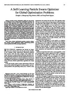
that solution. In Figure 1 we have graphically presented the rate of convergence of all the methods over four difficult test functions (in 60 dimensions). We have refrained from presenting all graphs in order to save space. A close inspection of Table 2 reveals that out of 16 test-cases, in 13 instances, IAPSO alone could achieve the minimum objective function value in a given number of FEs. Again, in 11 cases out of these 13, the difference of the means of IAPSO and the second best algorithm (which in most of the cases was CLPSO) remained statistically significant. We note that in three cases (f7 with D = 60, f8 with D = 30 and 60), the proposed method’s mean is numerically larger (i.e., worse) than the mean of the competitor (MPSO-TVAC or DE), but as the 10-th column of Table 2 shows, this difference is not statistically significant in the first two cases. Table 3 indicates that IAPSO could achieve better accuracies, consuming lesser amount of computational time. The overall results show that
the proposed method leads to significant improvements in most cases. Table 3 shows that the number of runs that converges below a pre-specified cut-off value is also greatest for IAPSO over most of the benchmark problems covered here. This indicates the higher
robustness (i.e. the ability to produce similar results over repeated runs on a single problem) of the algorithm as compared to its other four competitors. Usually in the community of stochastic search algorithms, robust search is weighted over the highest possible convergence rate
Table 3: Number of runs (out of 50) to optimality and the corresponding mean number of function evaluations
D
F
Threshold Value
BPSO
PSO-TVIW
MPSOTVAC
HPSOTVAC
CLPSO
IAPSO
1.00e-002
22, 9817.50 (8723.837)
50, 13039.65 (336.378)
50, 9410.04 (1231.278)
46, 6887.50 (22.281)
50, 37847.82 (4431.90)
50, 9492.64 (4371.276)
60
1.00e-002
16, 359834.33 (4353.825)
50, 51729.02 (3827.47)
50, 133282.72 (5326.366)
47, 136291.70 (238.944)
30
1.00e-002
0
0
0
0
50, 278283.22 (32432.78) 3, 203854.67 (3226.84)
50, 39928.40 (26431.627) 5, 79928.20 (12345.74)
60
1.00e-002
0
0
30
f1 f2 f3
f4
f5 f6
f7
f8
No. of runs converging to the cut-off, Mean No. of FEs Required and (Std Deviation)
0
0
0
0
5, 28372.40 (3225.63) 2, 733210.50 (4623.31) 50, 125092.84 (2473.98)
2, 26290.50 (7553.38)
6, 87812.83 (409.54)
0
0
18, 82724.46 (4523.57)
46, 92071.38 (4651.34)
50, 4883.78 (382.74) 50, 628389.73 (14383.82) 50, 3169.64 (761.65)
3, 633782.33 (1217.25)
2, 92280.50 (3468.35)
0
0
10, 129372.80 (8742. 93) 3, 664722.33 (4722.37) 0
8, 76660.00 (4412.46) 4, 89840.25 (6823.86) 0
0
0
0
0
0
0
0
0
0
0
0
0
0
0
0
30
1.00e-002
60
1.00e-002
0
0
30
1.00e-002
4, 9946.25 (314.821)
60
1.00e-002
2, 187635.50 (19224.46)
30
1.00e-002
50, 227361.76 (11354.287) 29, 287416.91 (7218.93) 6,347285.83 (3382.229)
60
1.00e-002
30
1.00e-002
60
1.00e-002
30
1.00e-002
60
1.00e-002
30
1.00e-002
60
1.00e-002
0
4, 139584.25 (2563.38) 2, 162258.50 (6922.83) 0
0
0
Fig 1a. Rosenbrock’s function (f2)
0
12, 80566.67 (7823.76) 0 24, 97276.67 (3517.88) 0
50, 6176.84 (671.49) 50, 3955.22 (451.89) 50, 4185.62 (447.81) 50, 5704.02 (728.45) 50, 6267.62 (265.82)
0
2, 126380.50 (4627.73)
0
0
0
6, 2400.50 (3712.5) 0
0
0 0
7, 7868.56 (251.67)
0
Fig 1.b Griewank’s function (f3)
Fig 1.c Ackley’s function (f5) Figure 1. Variation of the mean best value with time (for dimension = 60)
5. Conclusions This work has presented a new, efficient PSO algorithm, which self-adapts the inertia weight over different fitness landscapes. The new method has been compared against the basic PSO and four well-known PSO-variants, using an eight-function test suite, on the following performance metrics: (a) solution quality, (b) speed of convergence, and (c) frequency of hitting the optimum. It has been shown to outperform its nearest competitor in a statistically meaningful way for majority of the test cases. Since all the algorithms start with the same initial population, difference in their performances must be due to the difference in their internal operators and parameter values. Future research will focus on studying the dynamics of the particles under the proposed changes, in a mathematical way.
References [1] Kennedy, J., Eberhart, R. C: (1995) Particle swarm optimization, In Proceedings of IEEE International conference on Neural Networks. 1942-1948. [2] Kennedy, J., Eberhart, R. C., and Shi, Y.: (2001) Swarm Intelligence. Morgan Kaufman, USA. [3] Goldberg, D. E.: (1975) Genetic Algorithms in Search, Optimization and Machine Learning, Addison-Wesley, Reading, MA. [4] Kennedy, J.: (2003) Bare bones particle swarms, In Proceedings of IEEE Swarm Intelligence Symposium, 80-87. [5] Shi, Y. and Eberhart, R. C.: (1999) Empirical Study of particle swarm optimization, In Proceedings of IEEE International Conference Evolutionary Computation, Vol. 3 , 101-106. [6] Angeline, P. J.: (1998) Evolutionary optimization versus particle swarm optimization: Philosophy and
the performance difference, Lecture Notes in Computer Science, vol. 1447, Evolutionary Programming VII, 84-89. [7] Clerc, M. and Kennedy, J.: (2002) The particle swarm - explosion, stability, and convergence in a multidimensional complex space, In IEEE Transactions on Evolutionary Computation 6(1): 5873. [8] Kadirkamanathan, V., Selvarajah, K., and Fleming, P. J.: (2006) Stability analysis of the particle dynamics in particle swarm optimizer, IEEE Transactions on Evolutionary Computation vol.10, no.3, pp.245-255, Jun. 2006. [9] Shi, Y. and Eberhart, R. C.: (1998) A modified particle swarm optimizer, in Proc. IEEE Congr. Evol. Comput., 1998, pp. 69–73. [10] ____, (2001) Particle swarm optimization with fuzzy adaptive inertia weight, in Proc. Workshop Particle Swarm Optimization, Indianapolis, IN, 2001, pp. 101–106. [11] Ratnaweera, A., Halgamuge, K. S., and Watson, H. C.: (2004) Self organizing hierarchical particle swarm optimizer with time-varying acceleration coefficients, In IEEE Transactions on Evolutionary Computation 8(3): 240-254. [12] Liang, J. J., Qin, A. K., Suganthan, P. N., and Baskar, S.: (2006) Comprehensive learning particle swarm optimizer for global optimization of multimodal functions, IEEE Transactions on Evolutionary Computation, Vol. 10, No. 3, pp. 281295. [13] Mendes, R., Kennedy, J., and Neves, J.: (2004) The fully informed particle swarm: simpler, maybe better, IEEE Transactions on Evolutionary Computation., Vol. 8, no. 3, pp. 204-210, 2004. [14] Das, S., Konar, A., and Chakraborty, U. K.: (2005) Improving Particle Swarm Optimization with Differentially Perturbed Velocity, Proceedings of Genetic and Evolutionary Computation Conference (GECCO-2005), USA. [15] R. C. Eberhart, Y. Shi.: Particle swarm optimization: Developments, applications and resources, IEEE International Conference on Evolutionary Computation, vol. 1 (2001), 81-86. [16] Higashi, N., Iba, H.: (2003) Particle swarm optimization with Gaussian mutation, IEEE Swarm Intelligence Symposium , pp. 72-79. [17] Xie, X., F, Zhang, W., J., and Yang, Z, L. Adaptive particle swarm optimization on individual level, International Conference on Signal Processing (2002), 1215-1218. [18] Eberhart, R. C. and Shi, Y.: (2000) Comparing inertia weights and constriction factors in particle swarm optimization, IEEE International Congress on Evolutionary Computation, Vol. 1, 84-88. [19] van den Bergh, F, Engelbrecht, P. A., (2001) Effects of swarm size on cooperative particle swarm optimizers, In Proceedings of GECCO-2001, San Francisco CA, 892-899.