Jul 18, 2016 - In revenue management, the fundamental problem is the decision to find ... Many organizations use the overbooking policy. .... probability of consumer buy products when the price is t ...... [10] Chen, V., Gunther, D. and Johnson, E. (2003) Solving for an Optimal Airline Yield Management Policy via Statistical.
Open Journal of Social Sciences, 2016, 4, 1-9 Published Online July 2016 in SciRes. http://www.scirp.org/journal/jss http://dx.doi.org/10.4236/jss.2016.47001
Dynamic Pricing for Perishable Products with Control of Cancellation Demands and Strategic Consumer Hao Li, Meirong Tan, Liuxin Zou School of Economics and Management, Chongqing Jiaotong University, Chongqing, China Received 1 March 2016; accepted 18 July 2016; published 25 July 2016
Abstract In this paper, we consider the case that the consumers may cancel their reservations during the booking period so that consumers are divided into two parts: cancellation request and booking request. Simultaneously, we assume that consumers act strategically in booking products. Upon receiving the request, the firm has to decide whether to accept the cancellation request and what fees to charge the booking request in the presence of strategic consumers. We propose optimal price strategy and show the effectiveness of the decision models. We also obtain the optimal control of cancellation demands policy which is achieved by the number of remaining inventory. Numerical experiments are presented to explore the effect of various parameters on the performance of optimal strategy.
Keywords Control of Cancellation Demands, Revenue Management, Dynamic Pricing, Strategic Consumer
1. Introduction In revenue management, the fundamental problem is the decision to find the optimal price or inventory level in order to maximize total revenue. However, even though a good decision is made, a perfect match between predicted inventory and realized inventory still cannot be guaranteed. If realized inventory exceeds predicted inventory, some inventory will lose its value after the sale period. On the other hand, some consumers will become lost sales. Generally, the gap between predicted inventory and realized inventory comes from cancellation demand. In such circumstances, cancellation cause damage to firm’s sale that extra capacity becomes available and could be used to accommodate other potential consumers, which makes the system more complicated to operate. How could the firms to overcome this dilemma? Many organizations use the overbooking policy. Although this approach reduces the likelihood of being left with much unsold inventory, it may also lead to a difficult situation when the number of reservations exceeds the available inventory at the time of delivery. In such cases, the firm not only will lose the consumer but also damage the firm’s reputation. We present a possible business strategy in this paper. That is control of cancellation demand—whereby firm can decide whether or not accept a cancellation request in each period. The control of cancellation demands, combined with inventory vary dynamically, How to cite this paper: Li, H., Tan, M.R. and Zou, L.X. (2016) Dynamic Pricing for Perishable Products with Control of Cancellation Demands and Strategic Consumer. Open Journal of Social Sciences, 4, 1-9. http://dx.doi.org/10.4236/jss.2016.47001
H. Li et al.
makes the determination of how best to gain revenue become a difficult problem in the firm’s decision systems: How could the firm to charge price for the consumer who wants to buy an item? If a cancellation request arrives, whether or not accept her request? The models contained in this paper will help to answer these questions. Dynamic pricing models have been well studied in the literature. For reviews of pricing models for revenue management, please refer to Bitran and Caldentey (2003) [1], Levin and McGill (2009) [2] and Liu and Zhang (2013) [3], and for a survey of the literature that considers both pricing and inventory decisions, see Herk (1993) [4], Gallego and Van Ryzin (1994) [5], Elmaghraby and Keskinocak (2003) [6], Mahajan and Ryzin (2001) [7] and Kremer, Mantin, and Ovchinnikov (2015) [8]. In the stream of this work, a firm uses its price as a tool to induce demand, with the objective to maximize the total expected revenue when the sale ends. Because the optimal policy is often difficult to find analytically, in many cases the authors first establish structural properties of the optimal policy, and then develop an algorithm to compute or to approximate it. But these papers assume that consumers cannot cancel their reservations after purchasing. There are a number of the microeconomic literatures in existence, which focus on cancellation. Karaesmen and Van Ryzin (2004) [9] develop a cancellation-based model that exploits two-stage stochastic programs. Other approaches include: experimental designs and multi-variate adaptive regression splines (Chen et al., 2003) [10] in a DP setting, a sampling-based approach that combines merits of mathematical programming and an approximate DP algorithm for networks in which cancellations and over bookings are permitted (see Bertsimas and Popescu, 2003) [11]. Also, Gosavi et al. (2005) [12] provide a model-free simulation based optimization approach that can account for a variety of system-related assumptions, including arbitrary distributions for demand-arrival processes and cancellations. Schütz and Kolisch (2013) [13] model the problem as a Markov decision process in discrete time which due to proper aggregation can be optimally solved with an iterative stochastic dynamic programming approach. As far as we know, the existing literatures on the revenue management problems have not fully addressed flexible control of cancellation demand yet. The remainder of the paper is organized as follows. In the next two sections, we formulate our model and its associated dynamic programming value function. Section 4 analyzes the structure of the optimal policy and unfolds the basic property of the value function. A numerical example is presented in Section 5. We conclude with a brief discussion, as well as directions for future research in Section 6.
2. Model Descriptions We assume that the supplier has C units of a perishable product at the beginning of the sales season. The booking horizon is divided into T discrete time periods. The earliest period is period 0, and the last period is period T . We consider the case that the consumer may cancel their reservations during the booking period that extra capacity becomes available and could be used to accommodate other potential consumers. Based on the classification, there are two types of consumer: The first, we call it cancellation request, can be charged their service penalty, or they may be rejected. The second, we call it booking request, can be quoted prices that may vary dynamically. Also, we assume that these consumers are strategy. For strategic consumers, given price p at time t , they rationally anticipate purchase opportunities at future, and will buy at t only if the price is more attractive. The arriving consumer purchases products at time t only if the consumer’s utility of buying products at present time is greater than in the future. At any time t , the firm has to make the following decisions: 1) Accept or reject a cancellation request when a cancellation request arrives. 2) Charge fees of the booking request in the presence of strategic consumers. The supplier maximizes the expected revenue by simultaneously determining whether or not accept the cancellation request and the optimal prices for booking request in the presence of strategic consumers at any given time and remaining inventory. Figure 1 displays the decision procedure. The following notation is used throughout the paper: I : the number of remaining inventory; π : the refund per cancellation; p (t , I ) : price of a product in period t (simply denoted pt or p ); β : degree of strategic behavior of the consumer, β ∈ [0,1] . λ : probability of a consumer arrive, and λi be the probability of a type i arrive, where λ= λ1 + λ2 , i = 1, 2 .
2
H. Li et al. Accept
Cancellation request Firm checking Consumer arrive
Reject
Type Checking
Purchase
Firm checking
Purchase request
Dynamic pricing
Strategic consumers Wait
Figure 1. Two types of requests and the decision procedure.
χ (t , I , p, X ) : probability of consumer buy products when the price is pt and remaining inventory I (simply denoted χ t ). F ( X ) : cumulative probability distribution of the reservation price of a consumer, and f ( X ) be the common density function of F ( X ) . Let F (⋅) = 1 − F (⋅) . V (t , I ) : firm’s expected revenue over periods t to T if it follows the optimal cancellation control and dynamic pricing policy. u ( X − pt ) : consumer’s utility function to purchase products when the price is pt . We assume that all consumers have the same utility function, and u ( X − pt ) is the increasing of X − pt , where the inverse function is u −1 (⋅) , u ( X − pt ) ≥ 0 and u (0) = 0 . U (t , I , pt , X ) : consumer’s expected utility over periods t to T (simply denoted U (t , I ) ). Let us formally make some assumption for our model. 1) In each time-period t , no more than one request can arrive with probability λ ( λ= λ1 + λ2 ). No consumer arrival with probability 1 − λ1 − λ2 . 2) The refund per cancellation, π , is constant during the sale season. 3) The cumulative probability distribution of the reservation price of a booking request, F ( X ) , is continuously differentiable and increasing.
3. The Model Given price pt and remaining inventory I , consumer’s expected utility is:
= U (t , I ) max E X [ χ t u ( X − pt ) + β (1 − χ t ) U (t + 1, I )] χt
(1)
The boundary conditions of Equation (1) are: 1) U (T + 1, I ) = 0 , ∀I 2) U (t , 0) = 0 , ∀t In Equation (1), χ t u ( X − pt ) denotes consumer’s utility of buying products at present period; β (1 − χ t ) U (t + 1, I ) denotes consumer’s utility without buying products at present period. We can solve the maximize of U (t , I ) in χ t : when u ( X − pt ) ≥ U (t + 1, n) , χ t = 1 ; when u ( X − pt ) < U (t + 1, I ) , χ t = 0 , combine it ,we can obtain the optimal χ t :
E X [ χ (t , I , pt= , X )] E X [ I (u ( X − pt ) ≥ β U (t + 1, I ))]
(2)
where I (⋅) is indicator function Equation (2) means in any period t , only if consumer’s utility of buying products at present time is greater than in the future, the arriving consumer purchases products right now. Otherwise, choose to wait. Then, in any period t , given pt , we can obtain that:
E X [ χ (t , I , pt ,= X )] E X [ I ( X ≥ pt + u −1 ( β U (t + 1, I )))] = F ( pt + u −1 ( β U (t + 1, I ))) Let q (t , pt , I ) = pt + u −1 ( β U (t + 1, I )) , simply denoted qtI .
3
H. Li et al.
For each t and I , the expected revenu under optimality cancellation control and dynamic pricing policy can be expressed as: = V (t , I ) λ1 max{V (t + 1, I ), V (t + 1, I + 1) − π } + λ2 max{F (qtI )(V (t + 1, I − 1) + pt ) pt
+ (1 − F (q ) ⋅ V (t + 1, I )} + (1 − λ1 − λ2 )V (t + 1, I ) I t
I B , and by contradiction, suppose that pt* ( B) > pt* ( A) . Then F (qtI ( pt* ( A))) < F (qtI ( pt* ( B ))) , so
0 > F (qtI ( pt* ( A)))(− B + pt* ( A)) − F (qtI ( pt* ( B)))(− B + pt* ( B)) = F (qtI ( pt* ( A)))(− A + pt* ( A)) − F (qtI ( pt* ( B)))(− A + pt* ( B)) + ( B − A)( F (qtI ( pt* ( B))) − F (qtI ( pt* ( A))))
But the expression on the right-hand side is positive, which is a contradiction. = g ( B) F (qtI ( pt* ( B)))(− B + pt* ( A)) < F (qtI ( pt* ( B)))(− A + pt* ( B)) 2) Let A > B , ≤ F (qtI ( pt* ( A)))(− A + pt* ( A)) = g ( A) This completes the proof. Several revenue management models, such as Gallego and Van Ryzin (1994) [5], have shown that ∆V (t , I ) is increasing in I for any fixed t . We will prove this property in control of cancellation demands model in Equation (3). Theorem 2. ∆V (t , I ) is decreasing in I for any fixed t . Proof. Let ptI arg max{ F (qtI )(V (t + 1, I − 1) + ptI ) + (1 − F (qtI ))V (t + 1, I )} = I pt
ptI −1 arg max{ F (qtI −1 )(V (t + 1, I − 2) + ptI −1 ) + (1 − F (qtI −1 ))V (t + 1, I − 1)} = I −1 pt
= ptI +1 arg max{ F (qtI +1 )(V (t + 1, I ) + ptI +1 ) + (1 − F (qtI +1 ))V (t + 1, I + 1)} I +1 pt
For any fixed t ,
V2 (t , I + 1, p ) + V2 (t , I − 1, p ) − 2V2 (t , I , p) ≤ V (t + 1, I + 1) + V (t + 1, I − 1) − 2V (t + 1, I ) + F (qtI +1 )(2V (t + 1, I ) − V (t + 1, I + 1) + V (t + 1, I − 1)) + F (qtI −1 )(V (t + 1, I − 2) − 2V (t + 1, I − 1) + V (t + 1, I )) because p I maximizes V2 (t , I , p ) . So we have V2 (T , I + 1, p ) + V2 (T , I − 1, p ) − 2V2 (T , I , p ) ≤ 0 , which follows from the boundary conditions of Equation (3). The proof is by inverse induction on time. The basis for induction is the terminal conditions. When t = T ,
5
H. Li et al.
V= (T , I ) λ1V1 (T , I ) + λ2V2 (T , I ) + (1 − λ1 − λ2 )V (T + 1, I ) = λ1 max{V (T + 1, I ), V (T + 1, I + 1) − π } + λ2V2 (T , I ) = λ2V2 (T , I ).
V (T , I + 1, p ) + V (T , I − 1, p ) − 2V (T , I , p ) = λ2V2 (T , I + 1, p ) + V2 (T , I − 1, p ) − 2V2 (T , I , p ) ≤0 We can see that ∆V (T , I ) is decreasing in I for any fixed t . Suppose that the property is hold for t + 1, t + 2, , T . By assumption,
= V (t , I ) λ1 max{V (t + 1, I ), V (t + 1, I + 1) − π } + λ2V2 (t , I ) + (1 − λ1 − λ2 )V (t + 1, I ) Then: V2 (t , I + 1, p ) + V2 (t , I − 1, p ) − 2V2 (t , I , p )
≤ V (t + 1, I + 1) + V (t + 1, I − 1) − 2V (t + 1, I ) + F (qtI +1 )(V (t + 1, I ) − V (t + 1, I + 1) + ptI +1 ) + F (qtI −1 )(V (t + 1, I − 2) − V (t + 1, I − 1) + ptI −1 ) − F (qtI +1 )(V (t + 1, I − 1) − V (t + 1, I ) + ptI +1 ) − F (qtI −1 )(V (t + 1, I − 1) − V (t + 1, I ) + qtI −1 ) ≤0 Obviously, the expression on the right-hand side of V (t , I ) is concave in I at any fixed t . We conclude, by induction, that ∆V (t , I ) is decreasing in I for any fixed t . This completes the proof. Theorem 3. The optimal price satisfies the equation:
= pt*
1 − F (qtI ( pt* )) + ∆V (t , I ) . f (qtI ( pt* ))
(8)
(1 − F (qtI ) 2 is decreasing in p , then there exists a unique solution to V (t , I ) . f (qtI ) Proof. Taking the first derivative of V (t , I ) with respect to p yields:
Furthermore, if
∂V (t , I ) = λ2 [− f (qtI )(V (t + 1, I − 1) + pt ) + 1 − F (qtI ) + f (qtI )V (t + 1, I )]= 0 ∂p = pt*
1 − F (qtI ( pt* )) + ∆V (t , I ) . f (qtI ( pt* ))
The second derivative of V (t , I ) with respect to p is equal to:
∂ 2V (t , I ) = λ2 [− f ′ (qtI )(V (t + 1, I − 1) + pt ) − V (t + 1, I )) − 2 f (qtI )] 2 ∂p From Equation (9), we have:
(1 − F (qtI ) 2 is decreasing in p , so f (qtI )
Because
[
We have So if
f ′ (qtI )(1 − F (qtI )) ∂ 2V (t , I ) = − − 2 f (qtI ) f (qtI ) ∂p 2
(1 − F (qtI ) 2 1 − F (qtI ) f ′ (qtI )(1 − F (qtI )) − 2 f 2 (qtI ) f ′ (qtI )(1 − F (qtI )) − 2 f 2 (qtI ) ′ = − ⋅ − I * , V1 (t , I ) = V (t + 1, I − 1) , the firm reject the cancellation request. This completes the proof. The following corollary immediately follows from the optimal capacity control policy described in the above theorem. Corollary 3. The optimal threshold level for the cancellation request, I * , is a non-increasing function of π . Proof. We prove it by contradiction. Suppose that π 1 > π 2 . At any time t , the optimal threshold for π 1 is I1* , the optimal threshold for π 2 is I 2* . By contradiction, suppose that I1* > I 2* . From the definition of I 2* , we have V (t + 1, I 2* ) − V (t + 1, I 2* − 1) < π 2 < π 1 . Because V (t + 1, I1* ) − V (t + 1, I1* − 1) < V (t + 1, I 2* ) − V (t + 1, I 2* − 1) , V (t + 1, I1* ) − V (t + 1, I1* − 1) < V (t + 1, I 2* ) − V (t + 1, I 2* − 1) < π 2 < π 1
This contradicts the definition of I1* . Corollary 3 demonstrates that the higher the refund is, the lower I * for firm to accept or reject the cancellation request will be. The reason is also intuitive, when the price of products increases, it means that the profit for the firm will increase by offering products to cancellation request, as a result they will keep more products. Now we present a computation procedure for the optimal policy. The procedure leads to a closed-form solu-
7
H. Li et al.
tion which satisfies Equation (3). Moreover, as part of the control rules, all thresholds and price are jointly determined. We describe the recursive solution process as follows. First, we note V (T + 1, I ) = 0 for all I . Assume that V (t + 1, I ) , V (t + 1, I + 1) has been solved. Given the total number of selling units I , the optimal price can be determined through one-dimensional search, and I * can be obtained by Theorem 4. The condition I < I * implies that firm must accept the request for products. If I > I * , the firm reject the request of first type of consumer and provide the price p* . If the second type of consumer comes, the firm provides the price p* . The V (t , I ) can be solved by a backward recursion for the discrete time set with boundary condition V (T + 1, I ) = 0 , V (t , C ) = 0 .
5. Numerical Experiments We present a numerical experiment in this section to illustrate how the proposed approach works in a constructed example. X with T = 1000 , λ1 = 0.2 , λ2 = 0.4 . In all examples, the common density funcWe tested sets of examples 1 − tion f ( X ) is f ( X ) = e µ with mean µ . The mean µ is the average price a consumer would pay for µ McGill, 2009, [2]) We assume µ = 1 . We conduct numerical experiments which the product (see Levin and study the effects of the model on the performance of optimal strategy. First, we will illustrate the refund value π on the performance of I * , as demonstrated in Figure 2, wherein t = 900 , I = 100 . Three values of λ1 will be considered: 0.1, 0.4 0.8. Observer that, as proven by Corollary 3, I * is a non-increasing function of π . Also, we can see that I * is non-increasing in λ1 . The reason is intuitive, a large λ1 means the probability of cancellation request is large, there will be fewer cancellation inventory retained for those consumers in order to gain more profit trough dynamic pricing. Next, we consider the ratio of expected total revenue. The ratio is shown in Figure 3 as a function of I for T = 100 . We define that V (t , I ) − V ′(t , I ) = × 100 ρ V (t , I ) with V ′(t , I ) is define in Equation (6). 80
λ =0.1
70
1
λ =0.4
60
1
λ =0.8
I*
50
1
40 30 20 10 0 0
0.1
0.2
0.3
0.4
0.5 π
0.6
0.7
0.8
0.9
1
Figure 2. The optimal control threshold I * as a function of π for different values of λ1 . 6 5
ρ
4
I=50 I=70 I=100
3 2 1 0 0
0.1
0.2
0.3
0.4 λ1
0.5
0.6
0.7
Figure 3. The value of ρ as a function of λ1 for different type of I .
8
0.8
H. Li et al.
We can see that if the probability of cancellation request is increasing, the value of ρ will increasing. Also, we find that the value of ρ is increasing in the inventory level of I for any given λ1 .
6. Conclusions In this paper we research the control policy of cancellation demands in revenue management. By building multiperiod dynamic programming model, we obtained the price relation which meet to strategic consumers. In addition, we proved that the firms optimal revenue function and structure properties of pricing strategy. Finally, we use numerical experiments to explore the effect of various parameters on the performance of optimal strategy and show the effectiveness of the decision models. The results show that: 1) When the probability of cancellation request is large, there will be fewer cancellation inventory retained for those consumers in order to gain more profit trough dynamic pricing. 2) The control of cancellation demands model is no worse than the non-control of cancellation demands model with different type of I. Our research can provide theoretical basis for the optimal pricing decision to firms in control of cancellation demands. There are a number of important research avenues that can be pursued. How to decide the refund per cancellation? In this paper, we only take strategic consumer into booking products, we can explore the normal purchase in the presence of strategic consumers in the future.
Acknowledgements This work was supported by the National Natural Science Foundation of China (Grant No: 71402012), and the Natural Science Foundation of Education in Chongqing(KJ130402).
References [1]
Bitran, G. and Caldentey, R. (2003) An Overview of Pricing Models for Revenue Management. Manufacturing & Service Operations Management, 5, 203-229. http://dx.doi.org/10.1287/msom.5.3.203.16031
[2]
Levin, Y. and McGill, J. (2009) Dynamic Pricing in the Presence of Strategic Consumers and Oligopolistic Competition. Management Science, 55, 32-46. http://dx.doi.org/10.1287/mnsc.1080.0936
[3]
Liu, Q. and Zhang, D. (2013) Dynamic Pricing Competition with Strategic Customers under Vertical Product Differentiiation. Management Science, 59, 84-101. http://dx.doi.org/10.1287/mnsc.1120.1564
[4]
Herk, L. (1993) Consumer Choice and Cournot Behavior in Capacity-Constrained Duopoly Competition. Rand Journal of Economics, 24, 399-417. http://dx.doi.org/10.2307/2555965
[5]
Gallego, G. and Van Ryzin, G.J. (1994) Optimal Dynamic Pricing of Inventories with Stochastic Demand over Finite Horizons. Management Science, 40, 999-1020. http://dx.doi.org/10.1287/mnsc.40.8.999
[6]
Elmaghraby, W. and Keskinocak, P. (2003) Dynamic Pricing in the Presence of Inventory Considerations: Research Overview, Current Practices, and Future Directions. Management Science, 49, 1287-1309. http://dx.doi.org/10.1287/mnsc.49.10.1287.17315
[7]
Mahajan, S. and Van Ryzin, G. (2001) Inventory Competition under Dynamic Consumer Choice. Operations Research, 49, 646-657. http://dx.doi.org/10.1287/opre.49.5.646.10603
[8]
Kremer, M., Mantin, B. and Ovchinnikov, A. (2015) Dynamic Pricing in the Presence of Strategic Consumers: Theory and Experiment. Social Science Electronic Publishing.
[9]
Karaesmen, I. and van Ryzin, G. (2004) Overbooking with Substitutable Inventory Classes. Operation Research, 52, 83-104. http://dx.doi.org/10.1287/opre.1030.0079
[10] Chen, V., Gunther, D. and Johnson, E. (2003) Solving for an Optimal Airline Yield Management Policy via Statistical Learning. Journal of the Royal Statistical Society Series C, 52, 19-30. http://dx.doi.org/10.1111/1467-9876.00386 [11] Bertsimas, D. and Popescu, I. (2003) Revenue Management in a Dynamic Network Environment. Transp Sci, 37, 257277. http://dx.doi.org/10.1287/trsc.37.3.257.16047 [12] Gosavi, A., Ozkaya, E. and Kahraman, A.F. (2006) Simulation Optimization for Revenue Management of Airlines with Cancellations and Overbooking. Operations Research, 29, 21-38. http://dx.doi.org/10.1007/s00291-005-0018-z [13] Schütz, H.-J. and Kolisch, R. (2013) Capacity Allocation for Demand of Different Customer-Product Combinations with Cancellations, No-Shows, and Overbooking When There Is a Sequential Delivery of Service. Annul Operations Research, 206, 401-423. http://dx.doi.org/10.1007/s10479-013-1324-5
9
Submit or recommend next manuscript to SCIRP and we will provide best service for you: Accepting pre-submission inquiries through Email, Facebook, LinkedIn, Twitter, etc. A wide selection of journals (inclusive of 9 subjects, more than 200 journals) Providing 24-hour high-quality service User-friendly online submission system Fair and swift peer-review system Efficient typesetting and proofreading procedure Display of the result of downloads and visits, as well as the number of cited articles Maximum dissemination of your research work
Submit your manuscript at: http://papersubmission.scirp.org/