Dynamic Simulation of Electric Machines on FPGA Boards. Hao Chen, Song Sun, Dionysios C. Aliprantis, and Joseph Zambreno. Department of Electrical and ...
Dynamic Simulation of Electric Machines on FPGA Boards Hao Chen, Song Sun, Dionysios C. Aliprantis, and Joseph Zambreno Department of Electrical and Computer Engineering Iowa State University, Ames, IA 50011 USA Simulation Front-end
Abstract—This paper presents the implementation of an induction machine dynamic simulation on a field-programmable gate array (FPGA) board. Using FPGAs as computational engines can lead to significant simulation speed gains when compared to a typical PC computer, especially when operations can be efficiently parallelized on the board. The textbook example of a free acceleration followed by a step load change is used to outline the basic steps of designing an explicit Runge–Kutta numerical ordinary differential equation (ODE) solver on the FPGA platform. The FPGA simulation results and speed improvement are validated versus a Matlab/Simulink simulation.
System Specification
Application Analysis HW/SW Synthesis
SW Simulator
HW Accelerator Simulator
I. I NTRODUCTION A field-programmable gate array (FPGA) is a reconfigurable digital logic platform, which allows for the parallel execution of millions of bit-level operations in a spatially programmed environment. Research has been under way on the modeling and real-time simulation of various electrical power components using FPGAs as computational [1]–[6] and noncomputational [7], [8] devices. Herein, the goal is to implement an entire dynamic simulation of an induction machine on a single FPGA board, as fast as possible (i.e., without being constrained by the requirement of real-time simulation). Even though an induction machine has been selected, a similar process can be used to simulate other types of electric machinery. The textbook example of a free acceleration followed by a step load change is used to outline the basic steps of implementing an explicit fourth-order Runge–Kutta (RK4) numerical ordinary differential equation (ODE) solver on the FPGA platform. The individual mathematical operations required by numerical integration algorithms are generally simple in terms of required logic (additions and multiplications). Hence, hardware implementations can be used to increase efficiency by reducing the overhead introduced by software, thus leading to simulation speed gains of two orders of magnitude when compared to PCs. Moreover, complex systems requiring the simultaneous solution of numerous differential equations for simulation are inherently conducive to a parallel mapping to physical computational resources. Therefore, an FPGA becomes an attractive choice for simulating complex electrical power and energy systems. This paper presents initial work towards an “ultimate” goal of a fully functional FPGA-based simulation platform, as shown in Fig. 1. Herein, an induction machine model is designed This project was financially supported by the “CODELESS: COnfigurable DEvices for Large-scale Energy System Simulation” project, funded by the Electrical Power Research Center (EPRC) at Iowa State University.
High-Speed Link FPGA Boards
Host Workstation
Fig. 1.
Conceptual approach for FPGA-based simulation
using Very High Speed Integrated Circuit Hardware Description Language (VHDL), synthesized and verified using Xilinx Integrated Software Environment (ISE), and implemented on the FPGA development board using Xilinx Embedded Development Kit (EDK). II. I NDUCTION M ACHINE M ODEL The equations of a fifth-order squirrel-cage induction machine model in the stationary reference frame are given by [9]: s vqs = Rs isqs + p(Ls isqs + Lm i0s qr ) s vds
= 0=
0=
Rs isds Rr0 i0s qr 0 0s Rr idr
+ p(Ls isds + Lm i0s dr ) 0 0s − ωr (Lr idr + Lm isds ) + p(L0r i0s qr 0 0s s 0 0s + ωr (Lr iqr + Lm iqs ) + p(Lr idr Te =
P pωr = 2J (Te − TL ) s 0s 0.75P Lm (isqs i0s dr − ids iqr )
(1) + +
Lm isqs ) Lm isds )
(2) (3) (4) (5) (6)
d where p = dt is the differentiation operator; Rs and Rr0 are the stator and rotor resistances; Ls and L0r are the stator and s rotor inductances; Lm is the magnetizing inductance; vqs and s vds are the qd-axes stator voltages; isqs and isds are the qd-axes 0s stator currents; i0s qr and idr are the qd-axes rotor currents; Te is the electromagnetic torque; TL is the load torque; ωr is the rotor angular electrical speed; P is the number of poles; and J is the total rotor inertia. These equations are used to simulate an induction machine
Clock Signal (CLK)
Runge-Kutta ODE Solver x n−1 ← x n Torque
Step 6: Te (Eq. 6)
TL
Stator Voltage Input
xn
ODE Function f (t , x)
s v qds
x
⎡v s (t ) ⎤ s v qds = ⎢ qss ⎥ ⎣vds (t ) ⎦ ⎧ Step 1: t ← tn −1 ⎪ Step 2: t ← tn−1 + 0.5h ⎨ Step 3: t ← t + 0.5h n −1 ⎪ ⎩ Step 4: t ← tn−1 + h
Memory on Board
⎧ Step 1: ⎪ Step 2: ⎨ Step 3: ⎪ ⎩ Step 4:
⎧ Step 1: ⎪ Step 2: ⎨ ⎪ Step 3: ⎩ Step 4:
k1 k2 k3 k4
⎡ iqss ⎤ ⎢ s ⎥ ⎢ ids ⎥ x n = ⎢ iqr′s ⎥ ⎢ s⎥ ⎢ idr′ ⎥ ⎢ω ⎥ ⎣ r⎦
x ← x n−1 x ← x n−1 + 0.5hk 1 x ← x n−1 + 0.5hk 2 x ← x n−1 + hk 3
Fig. 2.
FPGA implementation of induction machine simulation
free acceleration (where TL = 0) followed by a step load change (where TL is stepped to its rated value). The machine is excited by a balanced sinusoidal three-phase voltage set, which is expressed in qd-axes variables as s 2 − 31 − 13 Vs cos(ωe t) 3 vqs s 2π 1 1 vds = 0 − √3 √3 Vs cos(ωe t − 3 ) v0s 1 1 1 Vs cos(ωe t + 2π 3 ) (7) 2 2 2 Vs cos(ωe t) = −Vs sin(ωe t) . 0 Note that the zero-axis voltage is zero, and can be neglected in this case. III. FPGA I MPLEMENTATION A. Simulation Architecture The transient response of the electric machine is obtained by the RK4 numerical integration algorithm [10]. This is a fixedstep explicit integration algorithm, which is based on simple numerical calculations (additions and multiplications), and is thus straightforward to implement on the FPGA. The RK4 method for the initial value problem (px = f (t, x), x(t0 ) = x0 ) is described by: xn = xn−1 + h6 (k1 + 2k2 + 2k3 + k4 ) tn = tn−1 + h
(8) (9)
where xn is the RK4 approximation of x(tn ) (i.e., the exact solution), h is the time step, and k1 = f (tn−1 , xn−1 )
Step 5:
Vector x n (Eq. 8) Update
(10)
k2 = f (tn−1 + 0.5h, xn−1 + 0.5hk1 ) k3 = f (tn−1 + 0.5h, xn−1 + 0.5hk2 ) k4 = f (tn−1 + h, xn−1 + hk3 ) .
(11) (12) (13)
From (1)–(6), the system of ODEs can be expressed in the form px = f (t, x) by s pi = Ai + Bvqds
pωr =
0.375P 2 Lm s 0s (iqs idr J
−
(14)
isds i0s qr )
−
P 2J TL
(15)
where � i = isqs s vqds
�T isds i0s i0s , qr dr � s � T s , = vqs vds L2
Rs − σL s
− σLsmL0 ωr r
L2 m ω 0 r A = σLLs LRr m s0 σLs Lr Lm − σL 0 ωr
Rs − σL s Lm σL0r ωr Lm Rs σLs L0r
r
1 σLs
0 B = − Lm σLs L0r 0
Lm Rr0 σLs L0r Lm σLs ωr R0 − σLr0 r − σ1 ωr
Lm − σL ωr s Lm Rr0 σLs L0r 1 σ ωr R0 − σLr0 r
,
0 1 σLs
0 − σLLsmL0
,
r
1−L2m /Ls L0r .
0s and σ = The state variables are isqs , isds , i0s qr , idr , s s and ωr . The input variables are vqs , vds , and TL . The output variable is Te given by (6). Herein, this output is only selected as an example to highlight the computational step of calculating outputs that depend on the model states. As shown in Fig. 2, four functional modules are used to establish the induction machine model. The ‘Stator Voltage Input’
s s module is responsible for the generation of vqs and vds . The ‘ODE Function’ and ‘Vector Update’ modules constitute the RK4 solver. The ‘Torque’ module implements the calculation of the ‘output’ (6). These modules have been developed using VHDL in ModelSim [11], which is a verification and simulation tool for VHDL designs. All variables and parameters are represented as signed fixed-point numbers with 24 bits representing the integral part, and 32 bits representing the fractional part. This provides a numerical range that can accommodate every variable involved in the simulation, with a resolution of 2−32 . Every RK4 iteration shown in Fig. 3 consists of six steps. The ‘ODE Function’ module executes the evaluation of (14) and (15). The ‘Vector Update’ module is responsible for the alteration of x in f (t, x) during step 2, 3 and 4, as well s s as the calculation of (8) in step 5. Since vqs and vds in (14) are dependent on the time t, the ‘Stator Voltage Input’ s s module should generate the appropriate vqs and vds for the s ‘ODE Function’ module. Specifically, vqs (tn−1 + 0.5h) and s vds (tn−1 + 0.5h) are generated during step 1 and stored for the usage of the ‘ODE Function’ module in step 2 and step 3, while s s vqs (tn−1 + h) and vds (tn−1 + h) are generated during step 3 and stored for the usage of the ‘ODE Function’ module in step 4 and step 1 of the next iteration. Note that the ‘Stator Voltage Input’ module and the ‘ODE Function’ module are executed in parallel in step 1. A similar parallel execution is also performed in step 3. On the other hand, the ‘ODE Function’ module and the ‘Vector Update’ module have to be executed in serial pattern because the inputs of one strictly depend on the outputs of the other. To design a sinusoidal function involved in the ‘Stator Voltage Input’ module, a look-up table approach is followed. The value of sin(x) is obtained from a 1000-element long lookup table, while cos(x) is obtained from the same table using an offset of π/2, which corresponds to a searching index offset of 250 in the look-up table. As shown in Fig. 4, the START signal (active high) starts the sin–cos function block, and the DONE signal (active high) signifies the end of operations. The operations are allocated in six clock cycles, as follows: 1 (a multiplication operation); calculate x 2π 1 obtain the fractional part of |x 2π |: xf ; calculate N xf , where N = 1000; obtain sin(|x|) from the look-up table, where the searching index is the integer part of N xf : xi ; 5. obtain cos(x) from the look-up table, where the searching index is xi +250; meanwhile, determine the value of sin(x) according to sin(|x|) and the sign of x; 6. write the values of sin(x) and cos(x) to the output ports.
1. 2. 3. 4.
The ‘ODE Function’ module shown in Fig. 5 includes three blocks. The ‘Matrix Calculation’ block which yields the matrix A (=[aij ]4×4 ) in (14) is implemented using one multiplier and one subtracter. The elements (a21 , a23 , a32 , a34 ) in A, which involve multiplications with ωr , are obtained from the multiplier. The other four elements (a12 , a14 , a41 , a43 ) also associated with ωr are easily obtained from the subtracter since each one is the opposite of a former multiplication
s v qds (tn−1 )
iteration n-1
x n−1 Step 1
ODE Function
Stator Voltage Input (13 Clock Cycles)
f (tn−1 , x n−1 ) (17 Clock Cycles)
k1 s v qds (tn−1 + 0.5h)
Step 2
Vector Update (9 Clock Cycles)
x n−1 + 0.5hk1
ODE Function
f (tn−1 + 0.5h, x n−1 + 0.5hk1 ) (17 Clock Cycles)
k2 Stator Voltage Input (13 Clock Cycles)
Step 3
Vector Update (9 Clock Cycles)
x n−1 + 0.5hk 2
ODE Function
f (tn−1 + 0.5h, x n−1 + 0.5hk 2 )
iteration n
(17 Clock Cycles)
k3 Step 4
Vector Update (9 Clock Cycles)
s v qds (tn−1 + h)
x n−1 + hk 3 ODE Function
f (tn−1 + 0.5h, x n−1 + hk 3 ) (17 Clock Cycles)
k4 Step 5
Vector Update (9 Clock Cycles)
x n Memory Step 6
s v qds (tn−1 + h)
Torque (5 Clock Cycles)
xn
on Board
Te (tn )
ODE Function
f (tn , x n )
iteration n+1
(17 Clock Cycles)
Fig. 3.
RK4 iteration process
DONE
CLK
sin-cos function
START x
sin(x) cos(x)
START
DONE
CLK 1
Fig. 4.
2
3
4
5
6
sin–cos function block
result. The remaining elements are stored in advance because they are constants. The evaluation of (14) is executed by the ‘Equation Group’ block, which is implemented using a 5-stage tree-shaped pipelined multiplier and adder structure, shown in Fig. 6 [12], [13]. The evaluation of (15) is executed by the ‘5th
s v qds
START_M
Matrix Calculation
ωr
(6 Clock Cycles)
DONE_G
Equation Group
A i
f1 , f 2 , f3 , f 4
}
(8 Clock Cycles)
f
ST0 START_M = 0 START_G = 0 START_E = 0
START = 1 START_M = 1 START_G = 0 START_E = 0
ST1 START_M = 0 START_G = 0 START_E = 0
DONE_M = 1 START_M = 0 START_G = 1 START_E = 1
ST2 START_M = 0 START_G = 0 START_E = 0
f5
CLK
i
DONE_E = 0
DONE
DONE_M
START
DONE_M = 0
START = 0
START_G
DONE_E = 1
i = ⎡⎣i
s qs
s ds
i
i′
s qr
i′ ⎤⎦ s dr
T
START_E
i
5th Equation (6 Clock Cycles)
TL
DONE_E
legend: state signals
Fig. 5.
bk v
Fig. 7.
⎡ b1 ⎢0 B=⎢ ⎢b2 ⎢ ⎣0 1 b1 = σ Ls
stage 2 (2 +) stage 3 (1 +) stage 4 (1 +)
b2 = −
store
DONE_G = 1 DONE = 1 DONE_G = 0
ai1 iqss ai 2 idss ai 3 iqr′s ai 4 idr′s
stage 1 (5 x)
ST3 START_M = 0 START_G = 0 START_E = 0
ST4 DONE = 0
ODE function module
A = ⎡⎣ aij ⎤⎦
stage 5 (store)
state transition condition signals
4×4
0⎤ b1 ⎥ ⎥ 0⎥ ⎥ b2 ⎦
Lm
σ Ls Lr′
START_G
State diagram of FSM for ODE function module
TABLE I X ILINX V IRTEX –5 XC5VLX110T R ESOURCES U SAGE S UMMARY
Logic Utilization Number of Slice Registers Number of Slice LUTs (Look Up Tables) Number of LUT-FF (Flip Flop) pairs Number of DSP48Es
Used 7722
Available 69120
27503
69120
28927
69120
55
64
DONE_G
completely independent. Note that the number of clock cycles required for the ‘ODE Function’ module is not 14 = 6 + 8 (as implied by Fig. 5) but 17 = 6 + 8 + 3 (as shown in Fig. 3), because the FSM introduces 3 extra clock cycles. A similar FSM is also used to coordinate the behaviors of the four modules in Fig. 2, and adds an overhead of 12 clock cycles per iteration, so that the total number of clock cycles per iteration is 121 = 17 + 9 + · · · + 9 + 5 + 12 (see Fig. 3).
CLK
i = 1, k = 1 v = vqss
5x
i = 2, k = 1 v = vdss i = 3, k = 2 v = vqss
i = 4, k = 2 v = vdss Fig. 6.
2+
1+
1+
store
5x
2+
1+
1+
store
5x
2+
1+
1+
store
5x
2+
1+
1+
store
B. Synthesis and Implementation 5-stage pipeline structure and operation
Equation’ block, which is implemented using one multiplier and one subtracter. A finite state machine (FSM) [14], shown in Fig. 7, is designed to coordinate the behaviors of these three blocks. The START and DONE signals (also shown in Fig. 5) correspond to the main ‘ODE Function’ module. Each internal block has its own operation-start signal (START x) and operation-end signal (DONE x), where ‘x’ can be either ‘M’ (‘Matrix Calculation’ block), ‘G’ (‘Equation Group’ block), or ‘E’ (‘5th Equation’ block). For example, START M is activated (START M = 1) as soon as START is active. After completing the matrix calculation, the ‘Equation Group’ block and the ‘5th Equation’ block are executed in a parallel pattern (START G and START E are activated at the same time) because these two blocks are
After the functionality and results of all modules designed using VHDL were validated in the ModelSim environment, the Xilinx ISE was used to develop, synthesize and verify the substantial top-level wrapper module together with the machine model. The target FPGA device was Xilinx Virtex-5 XC5VLX110T [15]. The post-place and route report presented the FPGA hardware resources usage as shown in Table I, and that the maximum frequency of the clock signal that can be applied is 89.735 MHz. Generally, the consumption of FPGA hardware resources increases with model complexity. Note that the entire design for the machine model must fit within the resource limitation of the target FPGA device. Otherwise, an FPGA device with more hardware resources should be chosen or the machine model should be redesigned in order to meet the requirement of the FPGA device. The final system was integrated on a XUPV5-LX110T development board [16], which features the XC5VLX110T device.
MPMC DDR2 SDRAM DDR2 SDRAM
MPMC Module Interface
plb_machine
TABLE II I NDUCTION M ACHINE AND VOLTAGE S OURCE PARAMETERS
SPLB
MicroBlaze DPLB
SPLB
DPLB
Rs Rr0 Ls L0r Lm
0.087 Ω 0.228 Ω 35.5 mH 35.5 mH 34.7 mH
P J ωe Vs Prated
4 1.662 Kg·m2 2π60 rad/s p 460 2/3 V 50 HP
mb_plb
Xilinx Virtex‐5 XC5VLX110T Bus Master
Bus Slave
MPMC: Multi‐Port Memory Controller SPLB: Slave Processor Local Bus DPLB: Data Processor Local Bus Fig. 8.
Implementation architecture
Besides FPGA logic blocks, this device has the embedded MicroBlaze soft processor whose software is written in C. The Xilinx EDK was used to co-design the software and hardware of the device. The architecture of this embedded system is shown in Fig. 8. The machine model was implemented in the FPGA hardware denoted by ‘plb machine.’ The software exchanges data with ‘plb machine’ through the CoreConnect Processor Local Bus (PLB) denoted by ‘mb plb.’ The MicroBlaze is the ‘master’ device on the ‘mb plb,’ while other devices are considered ‘slaves.’ The MicroBlaze generates the clock signal, and is responsible for coordinating data exchanges between the FPGA hardware and software. When the system starts up, the MicroBlaze sends an initialization signal and initial state values to the ‘plb machine.’ Then it launches the simulation, and begins controlling the execution of iterations, sending/updating the input data (i.e., TL ) to the ‘plb machine’ at the beginning of each time step calculation. The simulation output data (i.e., xn and Te ) are stored in the registers of ‘plb machine’ as soon as each iteration is completed. While the next iteration proceeds in the FPGA, the MicroBlaze reads the data from the registers, and writes it on the DDR2 memory embedded on the development board through ‘mb plb.’ In other words, the execution of iteration n + 1 in ‘plb machine’ takes place in parallel with the action of sending the data of iteration n to memory. IV. S IMULATION R ESULTS The parameters of the induction machine and voltage source used for simulation are shown in Table II. Based on the options provided by the Xilinx EDK, the Processor-Bus clock frequency was set to 66.67 MHz, a value less than the maximum clock frequency (89.735 MHz) in the post-place and route report of the Xilinx ISE. The simulation time-step h was 10−4 s. In this simple implementation, the simulation data were retrieved
from the memory at the end of each simulation using the Xilinx Microprocessor Debugger. The exact same machine model was also implemented in Matlab/Simulink. The verification of the results coming from the FPGA implementation was performed versus a Simulink simulation using the ODE23tb solver with a maximum time step of 10−5 s. Fig. 9 shows the transient response of all five state variables and the electromagnetic torque during free acceleration followed by a step load change (at t = 1 s) from both FPGA board and Simulink. The results from the FPGA are superimposed on the Simulink waveforms, but they are so close that differences cannot be distinguished. To compare simulation speed, we ran the simulation using the ODE45 and ODE23 integration algorithms of Simulink with maximum step size of 10−4 s (typically the two “simplest” available solvers), because they are implementations of the explicit Runge–Kutta algorithm, albeit of a variable-step nature. The simulation speed was further increased by using the ‘Accelerator’ mode of Simulink, which replaces normal interpreted code with compiled code. The simulation times on an Intel Core2 Duo 2.2 GHz computer were 2.7 s for ODE45, and 2.0 s for ODE23. The FPGA simulation time was 36.6 ms, which represents a speed-up of two orders of magnitude. The simulation time will be further decreased if the clock frequency can be set to a higher value, if the simulation time step h is increased, or if a lower order integration algorithm (e.g., the trapezoidal algorithm) is used. V. C ONCLUSION This paper presented the FPGA implementation of an induction machine dynamic simulation, using the RK4 numerical integration algorithm. The entire machine model has been developed using VHDL, synthesized, and implemented on an FPGA board. An optimal VHDL design should be sought for the purpose of economizing FPGA hardware resources, especially when the model has high complexity. A comparison between the simulation results from FPGA and Simulink demonstrates the validity of this implementation. Simulation speed gains of two orders of magnitude demonstrate the performance advantage of FPGAs compared to PC-based simulations. FPGAs represent an interesting possibility for simulating more complex electrical power and power electronics-based systems because of their flexibility, high processing rates and possibility to parallelize numerical integration computations.
i 0s qr (A)
i sds (A)
i sqs (A)
Simulink
FPGA
500 0 −500 0
0.2
0.4
0.6
0.8
1
1.2
1.4
1.6
1.8
2
0
0.2
0.4
0.6
0.8
1
1.2
1.4
1.6
1.8
2
0
0.2
0.4
0.6
0.8
1
1.2
1.4
1.6
1.8
2
0
0.2
0.4
0.6
0.8
1
1.2
1.4
1.6
1.8
2
0
0.2
0.4
0.6
0.8
1
1.2
1.4
1.6
1.8
2
0
0.2
0.4
0.6
0.8
1
1.2
1.4
1.6
1.8
2
500 0 −500
500 0
i0s dr (A)
−500
500 0 −500
ωr (rad/s)
400 200 0
Te (N·m)
2000 0
−2000
Time (s) Fig. 9.
Free acceleration characteristics of induction machine
R EFERENCES [1] M. Martar, M. Adbel-Rahman, and A.-M. Soliman, “FPGA-based realtime digital simulation,” in Int. Conf. Power Syst. Transients, Montreal, Canada, Jun. 2005. [2] P. Le-Huy, S. Gu´erette, L. A. Dessaint, and H. Le-Huy, “Real-time simulation of power electronics in power systems using an FPGA,” in Canadian Conf. Electr. Comp. Eng., May 2006, pp. 873–877. [3] ——, “Dual-step real-time simulation of power electronic converters using an FPGA,” in IEEE Int. Symp. Ind. Electron., Montreal, Canada, Jul. 2006, pp. 1548–1553. [4] J. C. G. Pimentel and H. Le-Huy, “Hardware emulation for real-time power system simulation,” in IEEE Int. Symp. Ind. Electron., Montreal, Canada, Jul. 2006, pp. 1560–1565. [5] J. C. G. Pimentel, “Implementation of simulation algorithms in FPGA for real time simulation of electrical networks with power electronics devices,” in IEEE Int. Conf. Reconfig. Comp. & FPGA’s, Sep. 2006, pp. 1–8. [6] G. G. Parma and V. Dinavahi, “Real-time digital hardware simulation of power electronics and drives,” IEEE Trans. Power Del., vol. 22, no. 2, pp. 1235–1246, Apr. 2007. [7] T. Maguire and J. Giesbrecht, “Small time-step (< 2µSec) VSC model
[8]
[9] [10] [11] [12] [13] [14] [15] [16]
for the real time digital simulator,” in Int. Conf. Power Syst. Transients, Montreal, Canada, Jun. 2005. C. Dufour, J. B´elanger, S. Abourida, and V. Lapointe, “FPGA-based realtime simulation of finite-element analysis permanent magnet synchronous machine drives,” in IEEE Power Electron. Spec. Conf., Jun. 2007, pp. 909–915. P. C. Krause, O. Wasynczuk, and S. D. Sudhoff, Analysis of Electric Machinery and Drive Systems, 2nd ed. IEEE Press, 2002. W. Gautschi, Numerical Analysis: An Introduction. Boston: Birkh¨auser, 1997. ModelSim User’s Manual Software Version 6.4a, Mentor Graphics Corporation, Wilsonville, Oregon. P. P. Chu, RTL Hardware Design Using VHDL: Coding for Efficiency, Portability, and Scalability. Hoboken, New Jersey: Wiley-Interscience, 2006. J. Cavanagh, Verilog HDL: Digital Design and Modeling. Boca Raton, Florida: CRC Press, 2007. V. A. Pedroni, Circuit Design with VHDL. Cambridge, Massachusetts: MIT Press, 2004. Xilinx Virtex-5 FPGA Data Sheet. [Online]. Available: http://www. xilinx.com/onlinestore/silicon/online store v5.htm XUPV5-LX110T User Manual. [Online]. Available: http://www.xilinx. com/univ/xupv5-lx110T-manual.htm