Una de las alternativas para desarrollar métodos dinámicos es el análisis ... sin embargo, el diseËno de un método que permita seguir la dinámica de los datos y ...
Dynamic Spectral Clustering based on Kernels
˜ Diego Hern´an Peluffo Ord´onez
National University of Colombia - Manizales Faculty of Engineering and Architecture Department of Electric Engineering, Electronics and Computing Science Manizales, Colombia 2013
Dynamic Spectral Clustering based on Kernels
˜ Diego Hern´an Peluffo Ord´onez
Thesis presented as a partial request for the degree of: Doctor of Engineering - Automatics
Director: Ph.D. C´esar Germ´an Castellanos Dom´ınguez
Research subject: Spectral Clustering and Dynamic Data Analysis Research Group: Digital Signal Processing and Recognition Group
National University of Colombia - Manizales Faculty of Engineering and Architecture Department of Electric Engineering, Electronics and Computing Science Manizales, Colombia 2013
Agrupamiento espectral de datos din´amicos
˜ Diego Hern´an Peluffo Ord´onez
Esta tesis se presenta como requisito parcial para optar al t´ıtulo de : Doctor en Inger´ıa - L´ınea de Autom´atica
Director: Prof. C´esar Germ´an Castellanos Dom´ınguez
Tema de investigaci´on: Agrupamiento espectral y an´alisis de datos din´amicos Grupo de investigaci´on: Grupo de control y procesamiento digital de se˜nales
Universidad Nacional de Colombia, sede Manizales Facultad de Ingenier´ıa y Arquitectura Departamento de Ingenier´ıa El´ectrica, Electr´onica y Sistemas Manizales, Colombia 2013
To my parents
A mis padres
Acknowledgements First, I would like to express my sincere gratitude to Prof. Germ´an Castellanos, who was the advisor to develop this work. I thank him for the continuous support of my study and research training, as well as for his motivation and immense knowledge. Undoubtedly, his guidance was a major factor to achieve this goal in terms of both research and writing of this thesis. Also, I want to thank the members of my thesis committee: Prof. Johan Suykens, PhD. Carlos Alzate, Prof. Claudia Isaza, Prof. Jos´e Luis Rodr´ıguez, and Prof. Mauricio Orozco. To all of them, thanks for their encouragement, insightful comments, revisions and constructive questions. Especially, my sincere thanks goes to Prof. Johan Suykens and PhD. Carlos Alzate for offering me the chance for an internship in their research group and guiding me working on suitable and interesting topics to deal with this thesis’ issues. Now I would like to post my thanks to all my fellow research group. Especially, I thank to Sergio Garc´ıa, Cristian Castro, Santiago Murillo, and Andr´es Castro for the helpful discussions, and support. I thank to them not only for academic matters but also for their friendship which encouraged me to finish this process. My heartfelt thanks goes for my great friend Yenny Berr´ıo. She always found a way to encourage me in hard moments, despite the circumstances, with kindness and support. Thanks also to all the people (teachers and friends) who helped me somehow with the writing review. Another special thanks goes to Julie (Yoly kitty) who is such as an angel to me. She encourages me in both personal and spiritual matters. Also, she helped a lot checking the manuscript writing. I thank my family: my parents Mario Peluffo and Guilnar Ordo˜nez, and my brother Mario Eduardo Peluffo, for supporting me spiritually throughout the course of this work and my whole life. Last but not the least, I thank God to provide me life, wisdom and strength to finish successfully this stage of my life.
This work was supported by the research project “Grupo de control y procesamiento digital de se˜nales” identified with code 20501007205.
Abstract The analysis of dynamic or time-varying data has emerged as an issue of great interest taking increasingly an important place in scientific community, especially in automation, pattern recognition and machine learning. There exists a broad range of important applications such as video analysis, motion identification, segmentation of human motion and airplane tracking, among others. Spectral matrix analysis is one of the approaches to address this issue. Spectral techniques, mainly those based on kernels, have proved to be a suitable tool in several aspects of interest in pattern recognition and machine learning even when data are time-varying, such as the estimation of the number of clusters, clustering and classification. Most of spectral clustering approaches have been designed for analyzing static data, discarding the temporal information, i.e. the evolutionary behavior along time. Some works have been developed to deal with the time varying effect. Nonetheless, an approach able to accurately track and cluster time-varying data in real time applications remains an open issue. This thesis describes the design of a kernel-based dynamic spectral clustering using a primaldual approach so as to carry out the grouping task involving the dynamic information, that is to say, the changes of data frames along time. To this end, a dynamic kernel framework aimed to extend a clustering primal formulation to dynamic data analysis is introduced. Such framework is founded on a multiple kernel learning (MKL) approach. Proposed clustering approach, named dynamic kernel spectral clustering (DKSC) uses a linear combination of kernels matrices as a MKL model. Kernel matrices are computed from an input frame sequence represented by data matrices. Then, a cumulative kernel is obtained, being the model coefficients or weighting factors obtained by ranking each sample contained in the frame. Such ranking corresponds to a novel tracking approach that takes advantages of the spectral decomposition of a generalized kernel matrix. Finally, to get the resultant cluster assignments, data are clustered using the cumulative kernel matrix. Experiments are done over real databases (human motion and moon covered by clouds) as well as artificial data (moving-Gaussian clouds). As a main result, proposed spectral clustering method for dynamic data proved to be able for grouping underlying events and movements and detecting hidden objects as well. The proposed approach may represent a contribution to the pattern recognition field, mainly, for solving problems involving dynamic information aimed to either tracking or clustering of data.
14
Keywords Dynamic or time-varying data, kernels, primal-dual formulation, spectral clustering, support vector machines
Resumen El an´alisis de datos din´amicos o variantes en el tiempo es un tema de gran inter´es actual para la comunidad cient´ıfica, especialmente, en los campos de reconocimiento de patrones y aprendizaje de m´aquina. Existe un amplio espectro de aplicaciones en donde el an´alisis de datos din´amicos toma lugar, tales como el an´alisis de v´ıdeo, la identificaci´on de movimiento, la segmentaci´on de movimientos de personas y el eguimiento de naves a´ereas, entre otras. Una de las alternativas para desarrollar m´etodos din´amicos es el an´alisis matricial espectral. Las t´ecnicas espectrales, principalmente aquellas basadas en kernels, han demostrado su alta aplicabilidad en diversos aspectos del reconocimiento de patrones y aprendizaje de m´aquina, incluso cuando los datos son variantes en el tiempo, tales como la estimaci´on del n´umero de grupos, agrupamiento y clasificaci´on. La mayor´ıa de los m´etodos espectrales han sido dise˜nados para el an´alisis de datos est´aticos, descartando la informaci´on temporal, es decir, omitiendo el comportamiento y la evoluci´on de los datos a lo largo del tiempo. En el estado del arte se encuentran algunos trabajos que consideran el efecto de la variaci´on en el tiempo, sin embargo, el dise˜no de un m´etodo que permita seguir la din´amica de los datos y agrupar los mismos en ambientes de tiempo real, con alta fidelidad y precisi´on, es a´un un problema abierto. En este trabajo de tesis se presenta un m´etodo de agrupamiento espectral basado en kernels dise˜nado a partir de un enfoque primal-dual con el fin de realizar el proceso de agrupamiento considerando la informaci´on din´amica, es decir, los cambios de secuencia de los datos a lo largo del tiempo. Para este prop´osito, se plantea un esquema de agrupamiento que consiste en la extensi´on de una formulaci´on primal-dual al an´alisis de datos din´amicos a trav´es de un kernel din´amico. El esquema se basa en un aprendizaje de m´ultiples kernels (MKL) y se denomina dynamic kernel spectral clustering (DKSC). El m´etodo DKSC usa como modelo de MKL una combinaci´on lineal de matrices kernel. Las matrices kernel se calculan a partir de una secuencia de datos representada por un conjunto de matrices de datos. Subsecuentemente, se obtiene una matriz acumulada de kernel de tal forma que los coeficientes o factores de ponderaci´on del modelo son considerados como valores de evaluaci´on de cada muestra del conjunto de datos o frame. Dicha evaluaci´on se hace a partir de un novedoso m´etodo de tracking que se basa en la descomposici´on espectral de una matriz kernel generalizada. Finalmente, para la obtenci´on de las asignaciones de grupo resultantes, los datos son agrupados usando la matriz acumulada como matriz kernel.
16 Para efectos de experimentaci´on, se consideran bases de datos reales (movimiento de humanos y la luna cubierta por nubes en movimiento) as´ı como artificiales (nubes Gaussianas en movimiento). Como resultado principal, el m´etodo propuesto comprob´o ser una buena alternativa para agrupar eventos y movimientos subyacentes as´ı como para detectar objetos ocultos en ambientes cambiantes en el tiempo. Este trabajo puede representar un significativo aporte en el a´ rea de reconocimiento de patrones, principalmente, en la soluci´on de problemas que implican datos din´amicos relacionados con tracking o agrupamiento de datos.
Palabras clave Agrupamiento espectral, datos din´amicos o variantes en el tiempo, formulaci´on primal-dual, kernels, m´aquinas de vectores de soporte.
Contents Acknowledgements
9
Abstract
13
Resumen
15
Contents
20
List of figures
22
List of tables
23
List of algorithms
24
Nomenclature
25
I.
27
Preliminaries
1. Introduction 1.1. Motivation and problem statement 1.2. Objectives . . . . . . . . . . . . . 1.2.1. General objective . . . . . 1.2.2. Specific Objectives . . . . 1.3. Contributions of this thesis . . . . 1.4. Manuscript organization . . . . .
. . . . . .
28 29 30 30 30 30 31
2. State of the art on spectral clustering and dynamic data analysis 2.1. Spectral clustering . . . . . . . . . . . . . . . . . . . . . . . . . . . . . . 2.2. Kernel-based clustering . . . . . . . . . . . . . . . . . . . . . . . . . . . . 2.3. Dynamic clustering . . . . . . . . . . . . . . . . . . . . . . . . . . . . . .
33 33 35 37
. . . . . .
. . . . . .
. . . . . .
. . . . . .
. . . . . .
. . . . . .
. . . . . .
. . . . . .
. . . . . .
. . . . . .
. . . . . .
. . . . . .
. . . . . .
. . . . . .
. . . . . .
. . . . . .
. . . . . .
. . . . . .
. . . . . .
. . . . . .
. . . . . .
18
Contents
II. Methods
38
3. Normalized cut clustering 3.1. Introduction . . . . . . . . . . . . . . . . . . . . . . . . . . . . . . . . . . 3.2. Basics of graphs . . . . . . . . . . . . . . . . . . . . . . . . . . . . . . . . 3.2.1. Graph . . . . . . . . . . . . . . . . . . . . . . . . . . . . . . . . . 3.2.2. Weighted graphs . . . . . . . . . . . . . . . . . . . . . . . . . . . 3.2.3. Properties and measures . . . . . . . . . . . . . . . . . . . . . . . 3.3. Clustering Method . . . . . . . . . . . . . . . . . . . . . . . . . . . . . . 3.3.1. Multi-cluster partitioning criterion . . . . . . . . . . . . . . . . . . 3.3.2. Matrix representation . . . . . . . . . . . . . . . . . . . . . . . . . 3.3.3. Clustering algorithm . . . . . . . . . . . . . . . . . . . . . . . . . 3.4. Proposed alternatives to solve the NCC problem without using eigenvectors 3.4.1. Heuristic search-based approach . . . . . . . . . . . . . . . . . . . 3.4.2. Quadratic formulation . . . . . . . . . . . . . . . . . . . . . . . .
39 39 39 40 40 40 41 42 42 43 49 49 53
4. Kernel spectral clustering 4.1. Introduction . . . . . . . . . . . . . . . . . . . . . . . . . . 4.2. Kernels for clustering . . . . . . . . . . . . . . . . . . . . . 4.2.1. Kernel function . . . . . . . . . . . . . . . . . . . . 4.2.2. Types of kernel functions . . . . . . . . . . . . . . . 4.3. Least-squares SVM formulation for kernel spectral clustering 4.3.1. Solving the KSC problem . . . . . . . . . . . . . . 4.3.2. Out-of-sample extension . . . . . . . . . . . . . . . 4.3.3. KSC algorithm . . . . . . . . . . . . . . . . . . . . 4.4. Proposed data projection for KSC . . . . . . . . . . . . . . 4.4.1. Out-of-sample extension of PKSC . . . . . . . . . . 4.4.2. Estimation of the lower dimension . . . . . . . . . . 4.4.3. PKSC algorithm . . . . . . . . . . . . . . . . . . .
. . . . . . . . . . . .
57 57 58 59 60 62 63 65 65 65 68 68 69
. . . . . . . . .
70 70 71 72 73 78 79 83 83 84
5. Proposed dynamic spectral clustering 5.1. Introduction . . . . . . . . . . . . . . . 5.2. Multiple kernel learning for clustering . 5.3. Tracking by KSC . . . . . . . . . . . . 5.3.1. Tracking vector . . . . . . . . . 5.3.2. KSC-based tracking algorithm . 5.3.3. Toy example: moving-curve . . 5.3.4. Links with relevance analysis . 5.4. Dynamic KSC . . . . . . . . . . . . . . 5.4.1. Dynamic KSC algorithm . . . .
. . . . . . . . .
. . . . . . . . .
. . . . . . . . .
. . . . . . . . .
. . . . . . . . .
. . . . . . . . .
. . . . . . . . .
. . . . . . . . .
. . . . . . . . .
. . . . . . . . .
. . . . . . . . .
. . . . . . . . . . . .
. . . . . . . . .
. . . . . . . . . . . .
. . . . . . . . .
. . . . . . . . . . . .
. . . . . . . . .
. . . . . . . . . . . .
. . . . . . . . .
. . . . . . . . . . . .
. . . . . . . . .
. . . . . . . . . . . .
. . . . . . . . .
. . . . . . . . . . . .
. . . . . . . . .
Contents
19
III. Experiments and results
85
6. Experimental setup 6.1. Considered database for experiments . . . . . . . . . . . . . . . . 6.1.1. Real databases . . . . . . . . . . . . . . . . . . . . . . . 6.1.2. Toy databases . . . . . . . . . . . . . . . . . . . . . . . . 6.1.3. Image database . . . . . . . . . . . . . . . . . . . . . . . 6.1.4. Video databases . . . . . . . . . . . . . . . . . . . . . . . 6.2. Clustering Performance Measures . . . . . . . . . . . . . . . . . 6.2.1. Supervised measures . . . . . . . . . . . . . . . . . . . . 6.2.2. Unsupervised measures . . . . . . . . . . . . . . . . . . . 6.2.3. Proposed performance measures . . . . . . . . . . . . . . 6.3. Experiment description . . . . . . . . . . . . . . . . . . . . . . . 6.3.1. Experiments for assessing the projected KSC performance 6.3.2. Experiments for KSC-based tracking . . . . . . . . . . . 6.3.3. Experiments for Dynamic KSC . . . . . . . . . . . . . .
. . . . . . . . . . . . .
86 86 86 88 90 90 91 91 94 95 98 98 98 100
. . . . . . . . . . .
103 103 103 105 107 110 110 112 113 121 121 125
7. Results and discussion 7.1. Results for experiments of projected KSC (PKSC) . . . . . . 7.1.1. Clustering Results of Three-Gaussian Data Sets . . . 7.1.2. Clustering Results on Artificial Data Sets . . . . . . 7.1.3. Clustering Results of Real Data . . . . . . . . . . . 7.2. Experimental results for DKSC based on MKL . . . . . . . 7.2.1. Results for KSC tracking . . . . . . . . . . . . . . . 7.2.2. Results for Three-moving Gaussian database . . . . 7.2.3. Results for DKSC . . . . . . . . . . . . . . . . . . 7.3. Results for proposed alternatives to NCC . . . . . . . . . . . 7.3.1. Experimental results for NCChs . . . . . . . . . . . 7.3.2. Experimental results for NCC quadratic formulation
IV. Final remarks
. . . . . . . . . . .
. . . . . . . . . . .
. . . . . . . . . . .
. . . . . . . . . . . . .
. . . . . . . . . . .
. . . . . . . . . . . . .
. . . . . . . . . . .
. . . . . . . . . . . . .
. . . . . . . . . . .
. . . . . . . . . . . . .
. . . . . . . . . . .
128
8. Conclusions and future work 129 8.1. Conclusions . . . . . . . . . . . . . . . . . . . . . . . . . . . . . . . . . . 129 8.2. Future work . . . . . . . . . . . . . . . . . . . . . . . . . . . . . . . . . . 130 8.3. Another important remarks . . . . . . . . . . . . . . . . . . . . . . . . . . 131
20
Contents
V. Appendixes
132
A. Kernel K-means
133
B. Links with normalized cut clustering B.1. Multi-cluster spectral clustering (MCSC) from two point of view B.2. Solving the problem by a difference: Empirical feature map . . . B.2.1. Gaussian processes . . . . . . . . . . . . . . . . . . . . B.2.2. Eigen-solution . . . . . . . . . . . . . . . . . . . . . . C. Links between KSC with normalized cut clustering C.1. Multi-cluster spectral clustering (MCSC) from two point of view C.2. Solving the problem by a difference: Empirical feature map . . . C.2.1. Gaussian processes . . . . . . . . . . . . . . . . . . . . C.2.2. Eigen-solution . . . . . . . . . . . . . . . . . . . . . .
. . . .
. . . .
. . . .
. . . .
. . . .
. . . .
. . . .
. . . .
. . . .
. . . .
. . . .
134 134 135 136 136
. . . .
137 137 138 139 139
D. Relevance Analysis for feature extraction and selection via spectral anal140 ysis D.1. Feature relevance . . . . . . . . . . . . . . . . . . . . . . . . . . . . . . . 141 D.2. Generalized case . . . . . . . . . . . . . . . . . . . . . . . . . . . . . . . 142 D.3. MSE-based Approach . . . . . . . . . . . . . . . . . . . . . . . . . . . . . 143 D.4. Q − α Method . . . . . . . . . . . . . . . . . . . . . . . . . . . . . . . . . 144 D.5. Results . . . . . . . . . . . . . . . . . . . . . . . . . . . . . . . . . . . . . 145 E. Academic discussion
152
Bibliography
155
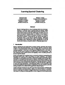
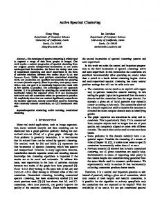
List of Figures 3.1. Weighted graph with three nodes . . . . . . . . . . . . . . . . . . . . . . . 3.2. Descriptive diagram of spectral clustering algorithm . . . . . . . . . . . . . 3.3. Heuristic search and graph . . . . . . . . . . . . . . . . . . . . . . . . . .
40 43 53
4.1. Feature space to high dimension . . . . . . . . . . . . . . . . . . . . . . . 4.2. High dimensional mapping . . . . . . . . . . . . . . . . . . . . . . . . . . 4.3. Accumulated variance criterion to determine the low dimension . . . . . .
58 60 68
5.1. Example of Dynamic Data . . . . . . . . . . . . . . . . . . . . . . . . . . 5.2. Graphic explanation of MKL for clustering considering the example of changing moon . . . . . . . . . . . . . . . . . . . . . . . . . . . . . . . . . . . 5.3. 2-D moving-curve . . . . . . . . . . . . . . . . . . . . . . . . . . . . . . . e = 3 clusters with N f = 100 frames 5.4. Clustering of 2-D moving-curve into K and N = 100 samples per frame . . . . . . . . . . . . . . . . . . . . . . . e = 4 clusters with N f = 100 frames 5.5. Clustering of 2-D moving-curve into K and N = 100 samples per frame . . . . . . . . . . . . . . . . . . . . . . .
71
6.1. 6.2. 6.3. 6.4. 6.5. 6.6. 6.7. 6.8. 6.9. 6.10. 6.11. 6.12. 6.13.
Examples of real data . . . . . . . . . . . . Motion Caption Database . . . . . . . . . . Subject #1 of Motion Caption Database . . 2D artificial databases . . . . . . . . . . . . Employed 3D databases . . . . . . . . . . . . . Three Gaussian Database . . . . . . . . . . Employed images . . . . . . . . . . . . . . Moon database . . . . . . . . . . . . . . . Example for explanation of PPQ measure three classes . . . . . . . . . . . . . . . . . Motion Caption Database . . . . . . . . . . Three Gaussian Database . . . . . . . . . . Subject #1 of Motion Caption Database . . Three-moving Gaussian clouds . . . . . . .
72 79 81 82
. . . . . . . . . . . . . . . . . 87 . . . . . . . . . . . . . . . . . 87 . . . . . . . . . . . . . . . . . 88 . . . . . . . . . . . . . . . . . 88 . . . . . . . . . . . . . . . . . 89 . . . . . . . . . . . . . . . . . 89 . . . . . . . . . . . . . . . . . 90 . . . . . . . . . . . . . . . . . 90 considering three clusters and . . . . . . . . . . . . . . . . . 96 . . . . . . . . . . . . . . . . . 99 . . . . . . . . . . . . . . . . . 99 . . . . . . . . . . . . . . . . . 101 . . . . . . . . . . . . . . . . . 101
22
List of Figures 7.1. Scatter plots for three-Gaussian data set with µ = [−0.3, 0, 0.3] and s = [0.1, 0.2, 0.3] (right column), and µ = [−1.8, 0, 1.8] and s = [0.1, 0.2, 0.3] (left column) . . . . . . . . . . . . . . . . . . . . . . . . . . . . . . . . . 7.2. Clustering performance for three-Gaussian data set with µ = [−1.8, 0, 1.8] and s = (0.1, 0.2, 0.3) . . . . . . . . . . . . . . . . . . . . . . . . . . . . . 7.3. HappyFace scatter plots for all studied methods for both training (left column) and test (right column) . . . . . . . . . . . . . . . . . . . . . . . . . 7.4. IRIS scatter plots for all studied methods for both training (left column) and test (right column) . . . . . . . . . . . . . . . . . . . . . . . . . . . . . . . 7.5. Dynamic analysis of Subject # 2 by KSC . . . . . . . . . . . . . . . . . . . 7.6. Clustering results for Subject # 2 . . . . . . . . . . . . . . . . . . . . . . . 7.7. Subject #2 tracking . . . . . . . . . . . . . . . . . . . . . . . . . . . . . . 7.8. Tracking Vectors for three-Gaussian moving . . . . . . . . . . . . . . . . . 7.9. Three-moving Gaussian regarding tracking-generated reference labels . . . 7.10. MKL weighting factors for Subject #1 . . . . . . . . . . . . . . . . . . . . 7.11. Clustering results for Subject #1 . . . . . . . . . . . . . . . . . . . . . . . 7.12. Clustering performance for three-moving Gaussian clouds . . . . . . . . . 7.13. Results over moon data set . . . . . . . . . . . . . . . . . . . . . . . . . . 7.14. Scatter plots for bullseye and happyface using the considered clustering methods . . . . . . . . . . . . . . . . . . . . . . . . . . . . . . . . . . 7.15. Clustering performance on image segmentation . . . . . . . . . . . . . . . 7.16. Clustering results after testing of considered databases . . . . . . . . . . . 7.17. Box plots of time employed for clustering methods. Improved MCSC at left hand and classical MCSC at right hand . . . . . . . . . . . . . . . . . . . . 7.18. Error bar comparing εM with the number of groups . . . . . . . . . . . . .
104 105 106 107 110 111 112 113 114 115 116 119 120 122 124 126 126 127
A.1. Graphically explanation of Kernel K-means for pixel clustering oriented to image segmentation . . . . . . . . . . . . . . . . . . . . . . . . . . . . . . 133 D.1. Relevance values for ‘E.coli’ data set. . . . . . . . . . . . . . . . . . . . . 147 D.2. Three first principal components of E.coli data set, applying each weighting method. . . . . . . . . . . . . . . . . . . . . . . . . . . . . . . . . . . . . 147 D.3. Classification percentage achieved with each weighting method performing feature extraction (applying PCA). A)No Weighting. B)PCA pre-normalization. C) Eigenvalues weighting. D)Q − α method. E)Q − b α method. F)ρ method. G)b ρ method. . . . . . . . . . . . . . . . . . . . . . . . . . . . . . . . . . . 147 D.4. Classification percentage achieved with each weighting method performing feature selection. A)No Weighting. B)PCA pre-normalization. C)Q − α method. D)Q − b α method. E)ρ method. F)b ρ method. . . . . . . . . . . . . 148
List of Tables 4.1. Kernel functions . . . . . . . . . . . . . . . . . . . . . . . . . . . . . . . .
61
5.1. Notation for the statement of theorems 5.3.1 and 5.3.2 . . . . . . . . . . . .
75
6.1. Real Data bases . . . . . . . . . . . . . . . . . . . . . . . . . . . . . . . . 6.2. contingency table for comparing two partitions . . . . . . . . . . . . . . .
86 93
7.1. 7.2. 7.3. 7.4. 7.5. 7.6. 7.7. 7.8. 7.9. 7.10. 7.11.
Overall results for considered real data . . . . . . . . . . . . . . . . . . . . Clustering performance for Subject # 2 in terms of considered metrics . . . Effect of number of groups over the Subject #2 . . . . . . . . . . . . . . . NMI and ARI for Subject # 1 clustering performance . . . . . . . . . . . . Clustering performance per frame for three-moving Gaussian clouds database Clusterings performance with PPQ along 10 iterations . . . . . . . . . . . Mean and standard deviation per cluster . . . . . . . . . . . . . . . . . . . Overall results for considered real and toy data along 10 iterations . . . . . Clustering performance with PPQ along 10 iterations . . . . . . . . . . . . Clustering processing time ratio along 10 iterations . . . . . . . . . . . . . Results for toy data sets . . . . . . . . . . . . . . . . . . . . . . . . . . . .
109 112 113 115 117 118 118 122 123 124 125
D.1. Notation used throughout this chapter . . . . . . . . . . . . . . . . . . . . 140 D.2. Classification performance applying feature extraction. Time correspond to the time needed to calculate the weighting vector, R% is the dimensionality reduction being 100% the original data set . . . . . . . . . . . . . . . . . . 150 D.3. Classification performance applying feature selection. . . . . . . . . . . . . 151
List of Algorithms 1. 2.
Normalized cut clustering . . . . . . . . . . . . . . . . . . . . . . . . . . . Heuristic Search for Clustering with prior knowledge and pre-clustering . .
48 54
3. 4.
Kernel spectral clustering: [qtrain , qtest ] = KSC(X, K(·, ·), K) Projected KSC: [qˆ train , qˆ test ] = PKSC(X, K(·, ·), K, p) . . . . � � e . . . . . . . . . . . KSCT: η = KSCT {X (1) , . . . , X (N f ) }, K n (t) oN f � � DKSC: qˇtrain = DKSC {X (1) , . . . , X (N f ) }, K(·, ·), K . . .
. . . . . . . . . . . . . . . .
65 69
. . . . . . . .
79
. . . . . . . .
84
5. 6. 7.
t=1
Q − α-based relevance analysis . . . . . . . . . . . . . . . . . . . . . . . . 145
Nomenclature Variables and functions Notation X K Ω U b U Z b Z e K
η Nf e Φ
dh b Φ n˜ e f H X e V e A λt u(t) Λ φ(·) K(·, ·) k·k ◦ tr(·) vec(·) ⊗
Denomination Description Data matrix X ∈ RN×d Number of clusters into data matrix K∈R Kernel or similarity matrix Ω ∈ RN f ×N f Rotation matrix U ∈ RN f ×N f b ∈ RN f טne Truncated rotation matrix U Projected data Z ∈ Rdh ×N f b ∈ Rdh טne Lower-rank projected data Z e∈R Number of clusters into frame matrix K Tracking vector η ∈ RN f Number of frames Nf ∈ R e ∈ RN f ×dh High dimensional representation matrix Φ High dimension dh >> d b ∈ RN f ×dh Reconstructed data matrix Φ Number of considered support vectors for frame matrix n˜ e ∈ N f Centering matrix for frame matrix H ∈ RN f ×N f Frame matrix X ∈ RN f ×Nd e ∈ RN f The degree matrix V e ∈ Rn˜ e Corresponding eigenvector matrix A The t–th eigenvalue of ΦΦT λt ∈ R T The t–th eigenvector of ΦΦ u(t) ∈ RN The Lagrange multipliers Λ ∈ RN×N Mapping function Kernel function Frobenius norm Hadamard product Trace Vectorization of its argument Kronecker product
26
List of Algorithms
Acronyms Term KSC DKSC MKL KSCT SVM LS-SVM PCA WPCA KPCA
Description Kernel spectral clustering Dynamic kernel spectral Clustering Multiple kernel learning KSC-based tracking Support vector machines Least-squares-Support Vector Machines Principal component analysis Weighted principal component analysis Kernel principal component analysis
Part I. Preliminaries
1. Introduction In the field of pattern recognition and classification, the clustering methods derived from graph theory and based on spectral matrix analysis are of great interest because of their usefulness for grouping highly non-linearly separable clusters. Some of its remarkable applications to be mentioned are human motion analysis and people identification [1, 2], image segmentation [3–5] and video analysis [6, 7], among others. The spectral clustering techniques carry out the grouping task without any prior knowledge –indication or hints about the structure of data to be grouped– and then partitions are built from the information obtained by the clustering process itself. Instead, they only require some initial parameters such as the number of groups and a similarity function. For spectral clustering, particularly, a global decision criterion is often assumed taking into account the estimated probability that two nodes or data points belong to the same cluster [8]. For this reason, this kind of clustering can be easily understood from a graph theory view point where such probability is to be associated to the similarity among nodes. Typically, clusters are formed in a lower dimensional space involving a dimensionality reduction process. This is done preserving the relationship among nodes as well as possible. Most approaches that deal with this matter are founded on linear combinations or latent variable models where the eigenvalue and eigenvector decomposition (here termed eigendecomposition) of the normalized similarity matrix takes place. In other words, spectral clustering comprises all the clustering techniques using information of the eigen-decomposition from any standard similarity matrix obtained from the data to be clustered. In general, these methods are of interest in cases where, because of the complex structure, clusters are not readily separable and traditional grouping methods fail. In the state of the art on unsupervised data analysis, we can find several approaches for spectral clustering. There are methods based on graph partitioning problems solved by a relaxed formulation that generally becomes a NP-complete problem [9–15]. These methods exploit the information given by the eigen-decomposition under the premise that any space generated by the eigenvectors (eigen-space) is directly related to the clustering quality [12]. Then, since it is possible to obtain a discrete solution, the muli-cluster clustering approach has emerged, named k-way normalized cuts [8]. Achieving such discrete solution implies to solve another clustering problem, albeit in a lower dimension. Therefore, the eigenvectors can be consid-
1.1 Motivation and problem statement ered as a new data set which can be grouped by means of a simple partitioning clustering method such as K-means [10]. The approach described in [10] corresponds to a recursive re-grouping method. However, the big disadvantage of this method is that it only works well when the information given by eigenvectors has a spherical structure [16]. Other works propose minimizing the difference between unconstrained problem solutions and some group indicators [17, 18] to find peaks and valleys of certain criterion capable of quantifying the group overlapping [19]. On the other hand, some spectral clustering approaches can be seen as particular cases of Kernel Principal Component Analysis (KPCA) as described in [20,21]. The work presented in [21] shows that conventional spectral clustering based on binary indicators, such as normalized cut [10], NJW algorithm [12] and random walk-based methods [9] are variants of weighted KPCA regarding different affinity matrices.
1.1. Motivation and problem statement In broad terms, clustering has shown to be a powerful technique for grouping and/or rank data as well as a proper alternative for unlabeled problems. Due to its versatility, applicability and feasibility, it has been preferred in many approaches. Nevertheless, despite several clustering techniques having been introduced, the selection and design of a grouping system is not a trivial task. Often, it is mandatory to analyze in detail the structure of data and the specific initial conditions of the problem in order to group the homogenous data points. Besides, it must be done in such a way that an accurate cluster recognition is accomplished. One of the biggest disadvantages of the spectral clustering methods is that most of them have been designed for analyzing only static data, that is to say, regardless of the temporary information. Therefore, when data are changing along time, clustering can be performed on single current data frame without analyzing the previous ones. Some works have addressed this important issue concerning applications such as human motion analysis [22, 23]. Other approaches are focused on the design of dynamic kernels for clustering [24,25] as well as the use of dynamic KPCA [26, 27]. In the literature, many approaches prioritize the use of kernel methods since they allow to incorporate prior knowledge into the clustering procedure. However, the design of a whole kernel-based clustering scheme able to group time-varying data achieving a high accuracy is still an open issue. This thesis presents the design of a kernel-based dynamic spectral clustering using a primaldual approach so as to carry out the grouping task involving the dynamic information, that is to say, the changes of data frames along time. To this end, a dynamic kernel-based approach to extend a simple primal formulation to dynamic data analysis is introduced. This approach may represent a contribution to pattern recognition mainly in applications involving timevarying information such as video analysis and motion detection, among others.
29
30
1 Introduction
1.2. Objectives 1.2.1. General objective To develop a whole kernel-based clustering scheme using a primal-dual formulation for grouping time-varying data.
1.2.2. Specific Objectives * To propose a kernel spectral clustering approach with a proper selection and/or tuning of initial parameters to group both complex and simple data. * To design a dynamic multiple kernel framework able to capture the evolutionary information in time-varying data. * To develop a whole clustering scheme based on kernels for grouping time-varying data frames via a primal-dual formulation.
1.3. Contributions of this thesis This thesis was done within the framework of clustering, specifically, spectral clustering based on kernels, yielding the following main contributions to the state of art on this field: • A new data projection to improve the performance of kernel spectral clustering is proposed. This projection consists of a linear mapping based on the M-inner product approach, for which an orthonormal eigenvector basis is chosen as the projection matrix. Moreover, projection matrix is calculated over the spectrum of kernel matrix. The strength of this approach is that local similarities and global structure are used to refine the projection procedure by preserving the most explained variance and reaching a projected space that improves the clustering performance within the KSC framework. Another advantage of the proposed data projection is that a more accurate estimation of the number of groups is provided. Since introduced projected KSC is derived from a support vector machine-based model, it can also be trained, validated, and tested in a learning framework using a model selection criterion. • A novel tracking approach based on the eigenvector decomposition of the normalized kernel matrix is proposed, which yields a ranking value for each single frame from the analyzed input sequence. As a result, obtained ranking values present a direct relationship with the underlying dynamic events contained in the sequence. This approach also provides substantial information to estimate both the number of groups and the ground truth.
1.4 Manuscript organization • Based on a multiple kernel learning approach, namely a linear of combination of kernels, a dynamic kernel spectral clustering (DKSC) approach is introduced. DKSC, from a set of kernels representing to a data matrix sequence, perform the clustering process over the input data using a cumulative kernel matrix obtained from the considered MKL approach. The weighting factors or coefficient for linear combination are those ranking values given by a proposed tracking approach. Then, proposed method is able to cluster dynamic data taking into account the past information. Also, this work achieved other additional contributions on related topics, which are not among the main topics but still important in the field of clustering: • Two novel alternatives to the conventional spectral normalized cut clustering (NCC) without using eigenvectors are introduced. One based on a piecewise heuristic search to determine the nodes having maximum similarity. Another one that consists of a variation of the NCC formulation aimed to pose a relaxed quadratic problem, which can be easy solved, for instance, by means of a conventional quadratic programming algorithm. Both proposed methods spend lower computational cost in comparison with conventional spectral clustering methods and keep a comparable performance as well. • A new supervised index for clustering performance, named probability-based performance quantifier (PPQ) is introduced. PPQ is based on simple probabilities calculated by relative frequencies and provides a relative value for each class from data base via the Bayes’ rule.
1.4. Manuscript organization The manuscript is divided into five parts, namely, I preliminaries, II methods, III experiments and results, IV final remarks, and V appendices. It is composed by eight main chapters, which are organized as follows: • Chapter 2 is a brief state of the art on kernel-based clustering for dynamic data. • In chapter 3, the normalize cut clustering (NCC) criterion from a graph-partitioning point of view is presented, aimed to solving multi-cluster problems via an eigenvector decomposition. Some alternatives to solve the NCC problem without using eigenvectors are introduced as well. • One of the capital chapters is chapter 4, in which the description of the kernel spectral clustering method is presented. Also, an optimal data projection for KSC is introduced. In addition, some definitions and basics about kernels are studied.
31
32
1 Introduction • Chapter 5 is the central chapter, which explains the dynamic version of KSC based on multiple kernel learning (MKL). Also, a tracking approach is introduced. • The experimental setup and results of this thesis are shown respectively in chapters 6 and 7. • In chapter 8, the conclusions achieved with this work and future work are presented.
2. State of the art on spectral clustering and dynamic data analysis Spectral clustering, just as any unsupervised technique, is a discriminative method, that is, it does not require prior knowledge about the classes for classification. As such, it performs the grouping process using only the information within the data and, generally, some starting parameters such as the number of resulting groups or any other hint about the initial partition. In this case, given that the spectral clustering is backed up by graph theory, the input parameters for clustering algorithms are the number of groups and the similarity matrix. The initialization is an important stage in the unsupervised methods since most of them are sensitive to the starting parameters; this means that if the initial parameters are not adequate, algorithm convergence may fail by falling on a suboptimal solution quite distant from the global optimum. On the other hand, as mentioned above, the unsupervised methods carry out the clustering with the direct information given by the data. Thus, if the initial representation space is not discriminative enough under the clustering criteria, feature extraction and/or selection stages may be, in some cases, required. Following, a brief theoretical background with a bibliographic scope on spectral clustering based on kernels is presented.
2.1. Spectral clustering Clustering based on spectral theory is a relatively new focus for unsupervised analysis; although it has been used in several studies that prove its efficiency on grouping tasks, especially in cases when the clusters are not linearly separable. This clustering technique has been widely used in a large amount of applications such as circuit design [9], computational load balancing for intensive computing [28], human motion analysis and people identification [1, 2], image segmentation [3–5] and video analysis [6, 7], among others. What makes spectral analysis applied to data clustering appealing is the use of the eigenvalue and eigenvector decomposition in order to obtain the local optima closest to the global continuous
34
2 State of the art on spectral clustering and dynamic data analysis optima. The spectral clustering techniques take advantage of the topology of data from a non-directed and weighted graph-based representation. This approach is known as graph partitioning; in it an initial optimization problem is usually posed formulated under some constraints. Often this formulation is relaxed and then becomes a NP-complete problem [9–14]. In addition, the estimation of global optima in a relaxed continuous domain is done through the eigenvector decomposition (eigen-decomposition) [8], based on the theorem by Perron - Frobenius, which establishes that largest strictly real eigenvalues associated to a positive definite and irreducible matrix determine their own spectral ratio [29]. In this case, such matrix corresponds to the affinity or similarity matrix containing the similarities among data points. In other words, the space created by the eigenvectors in the affinity matrix is closely related to the clustering quality. Under this principle, and considering the possibility of obtaining a discreet solution through eigenvectors, there have been proposed multi-cluster approaches such as the k-way normalized cut method introduced in [8]. In such method, to obtain the discrete solution, another optimization problem must be solved, albeit in a lower dimensional domain. Besides, leading eigenvectors can be considered as a new data set that can be clustered by a conventional clustering algorithm such as K-means [10, 30]. Then, a hybrid algorithm is achieved in which the spectral analysis algorithms may generate the eigenvector space and set adequate initial parameters, while partitioning algorithms would be in charge of the clustering itself. This means that the spectral analysis can support the conventional techniques generating an initialization improving the algorithm convergence. Nevertheless, similar to the hard membership values obtained from some center-based clustering algorithms [31], a spectral clustering scheme can cluster data alone outputting a cluster binary matrix denoting the data point membership regarding each cluster. To carry out this clustering approach, not only are the eigenvectors needed, but also is the orthonormal transformation of eigenvector solution (eigen-solution). This leads to the target of spectral clustering being the finding of the best orthonormal transformation that generates an appropriate discretization of the continuous solution [10]. In general, when dealing with bi-cluster problems, the solution of the relaxed problem is often a specific eigenvector [16]. However, when the problem is within a kind of multi-cluster framework, determining relevant information for the clustering task based on the eigensolution is not that simple. Among the approaches proposed to address the multi-way spectral clustering problem, we find recursive re-clustering methods (recursive-cuts) to obtain the cluster indicator vector as discussed in [10]. This approach is not optimal since it only takes into consideration an eigenvector and discards the information from the remaining vectors,
2.2 Kernel-based clustering which can also provide a clue as to the cluster conformation. The re-clustering approach amounts to applying a partitioning clustering method on the eigenvector space, although this only works properly when the eigen-space has a spherical structure [16]. In [30], authors propose a simple clustering algorithm consisting of a conventional method to estimate the most representative data points, one per cluster. This is done through the eigen-decomposition of the normalized similiraty matrix. Subsequently, an amplitude–re-normalized eigenvector matrix is obtained, which is clustered into K subsets using the K-means algorithm. Finally, the data points are assigned to the corresponding clusters according to the geometric structure of the initial data matrix. A later work [8] presents a method for multi-cluster spectral clustering in a more detailed manner, in which an optimization problem is posed to guarantee that the algorithm convergence lies within the global optimum region. To this end, two optimization sub-problems are formulated: one to obtain the global optimal values in an unconstrained continuous domain and another for getting a discrete solution corresponding to the continuos one. Unlike the algorithm introduced in [30], this method does not require an additional clustering algorithm since it generates a binary matrix on its own representing the data point membership. In this way each data point belong to an unique a cluster. In this study, orthonormal transformations and singular value decomposition are employed to determine the optimal discrete solution, taking into consideration the principle of orthonormal invariance and the optimal eigen-solution criterion. Another study [32] applies the foundations from [8] and [30] to explain theoretically the relationship between kernel K-means and spectral clustering, starting from the point of view of K-means objective function generalization towards obtaining a special case of the objective function able to solve the normalized cut (NC) problem. Then, a positive definite similarity matrix is assumed as well as algorithms based on local searches and optimization formulations are performed to improve the clustering process regarding the kernel. This is done in such a manner that it might be satisfied the optimization condition establishing that NC-based clustering objective function must be monotonically decreasing.
2.2. Kernel-based clustering More advanced approaches propose minimizing a feasibility measure between the solutions of the unconstrained problem and the allowed cluster indicator [17, 18], finding peaks and valleys of a cost function that quantifies the cluster overlapping [19]. Then, a discretization process is carried out. The problem of continuos solution discretization is formulated and solved in [33]. There exist graph-based methods associated with normalized and nonnormalized Laplacian, which provide relevant information contained in the Laplacian eigenvector is of great usefulness for the clustering task. As well, they often provide a straight-
35
36
2 State of the art on spectral clustering and dynamic data analysis forward interpretation about the clustering quality based on a random graph theory. Under the assumption that data is a random weigthed graph, it is demonstrated that spectral clustering can be seen as a maximal similarity-based clustering. In [18], some alternatives to solving open issues in spectral clustering are discussed, such as the selection of a proper analysis scale, extensions to multi-scale data management, the existence of irregular and partially known groups, and the automatic estimation of the number of groups. The authors propose a local scaling to calculate the affinity or similarity between each pair of data points. This scaled similarity improves the clustering algorithms in terms of both convergence and processing time. Additionally, taking advantage of the underlying information given by eigenvectors is suggested to automatically establish the number of groups. The output of this algorithm can be used as a starting point to initialize partitioning algorithms such as K-means. There are another approaches that have been pointed out to extend the clustering model to new data (testing data), i. e., out-of-sample extension. For instance, the methods presented in [34, 35] allow for extending the clustering process to new data, approximating the eigen-function (a function based on the eigen-decomposition) using the Nystr¨om’s method [36, 37]. Therein, a clustering method and a searching criterion are typically chosen in a heuristic fashion. Another spectral clustering perspective is the Kernel Principal Component Analysis (KPCA) [20, 21]. KPCA is an unsupervised technique for nonlinear feature extraction and dimensionality reduction [38]. Such method is a nonlinear version of PCA using positive definite matrices whose aim is to find the projected space onto an induced kernel feature space preserving the maximum explained variance [16]. The relationship between KPCA and spectral clustering is explained in [20, 21]. Indeed, the work presented in [21] demonstrates that the classical spectral clustering, such as normalized cut [10], the NJW algorithm [12] and random walk model [9] can be seen as particular cases of weighted KPCA, just with modifications on the kernel matrix. In [16], a spectral clustering model is proposed which is based on a KPCA scheme on the basis of the approach proposed in [21] in order to extend it to multi-cluster clustering, wherein coding and decoding stages are involved. To that end, a formulation founded on least squares method-based support vector machines (LSSVM) considering weighted versions [39, 40]. This formulation aims to a constrained optimization problem in a primal-dual framework that allows for extending the model to new isolated data without needing additional techniques (e. g. the Nystr¨om method). In this connection, a modified similarity matrix is proposed whose eigenvectors are dual regarding a primal optimization problem formulated in a high dimensional space. Also, it is proven that such eigenvectors contain underlying relevant information useful for clustering purposes and display a special geometric structure when the resulting clusters are well formed -in terms of compactness and/or separability.
2.3 Dynamic clustering The out-of-sample extensions are done by projecting cluster indicators onto the eigenvectors. As a model selection criterion, the method so-called Balanced Line Fit (BLF) criterion is proposed. This criterion explores the structure of the eigenvectors and their corresponding projections, which can be used to set the initial model parameters. Similarly, in [41], another kernel model for spectral clustering is presented. This method is based on the incomplete Cholesky decomposition. It is able to deal efficiently with largescale clustering problems. The set-up is made on the basis of a WPCA scheme based on kernels (WKPCA) from a primal-dual formulation. In it, the similarity matrix is estimated by using the incomplete Cholesky decomposition.
2.3. Dynamic clustering Dynamic data analysis is of great interest, there are several remarkable applications such as video analysis [42] and motion identification [43], among others. By using spectral analysis and clustering, some works have been developed taking into account the temporal information for the clustering task, mainly in segmentation of human motion [22, 23]. Other approaches include either the design of dynamic kernels for clustering [24, 25] or a dynamic kernel principal component analysis (KPCA) based model [26,27]. Another study [44] modifies the primal functional of a KPCA formulation for spectral clustering to add the memory effect. There exists another alternative known as multiple kernel learning (MKL), which has emerged to deal with different issues in machine learning, mainly, regarding support vector machines (SVM) [45, 46]. The intuitive idea of MKL is that learning can be enhanced when using different kernels instead of an unique kernel. Indeed, local analysis provided by each kernel is of benefit to examine the structure of the whole data when having local complex clusters.
37
Part II. Methods
3. Normalized cut clustering 3.1. Introduction The clustering methods based on graph partitioning are discriminative approaches to grouping homogeneous nodes or data points without making assumptions about the global structure of data, but local evidence on a pairwise relationship among data points is considered. Such relationship, known as similarity, defines how likely two data points are to belong to the same cluster. Then, all data points are split into disjunct subgraphs or subsets according to a similarity-based decision criterion. Most of approaches apply such criterion on a lowerdimensional space representing the original one, preserving the relationships among nodes as accurately as possible. Then, within a relaxed formulation, some feasible continuous solutions can be obtained by eigenvector decompositions [8]. Indeed, eigenvectors can be interpreted as geometric coordinates in order to directly cluster them by means of a conventional clustering technique as suggested in [18, 32]. Nonetheless, there are alternatives to achieve this clustering without using eigenvectors but taking advantages of multi-level schemes [47] or formulating easy-to-solve quadratic problems with linear constraints [15, 48]. In this work, we give special attention to the multi-cluster spectral clustering (MCSC) introduced in [8], since it computes a discrete solution from the space spanned by the eigenvectors regarding a certain orthonormal basis. Then, instead of using additional clustering stages, the MCSC generates some binary cluster indicators directly. The scope of this chapter encompasses a detailed explanation, formulation and solutions for the normalized cut clustering. We start mentioning some basics of graphs in section 3.2. Then, the MCSC method is described in section 3.3, by deriving a muti-cluster partitioning criterion from a graph theory point of view, as shown in section 3.3.1. The algorithm for MCSC is summarized in section 3.3.3.
3.2. Basics of graphs As mentioned above, a way to easily understand the spectral clustering methods is from a geometric perspective using graphs. In this section, some definitions around graphs are presented as well as properties and operations needed for further analysis.
40
3 Normalized cut clustering
3.2.1. Graph A graph is a non-empty finite set of nodes or data points, and edges connecting the nodes pairwise. Then, a so-called graph G can be described by the ordered pair G = (V, E), where V is the set of nodes and E is the set of edges.
3.2.2. Weighted graphs A weighted graph can be represented as G = (V, E, Ω), where Ω represents the relation among nodes, in other words, the affinity or similarity matrix. Given that Ωi j represents the weight of the edge between i-th and j-th node, it must be a non-negative value. In addition, in a non-directed graph is verified that Ωi j = Ω ji . Therefore, matrix Ω must be chosen as symmetric and positive semidefinite. Figure 3.1 shows an example of a weighted graph. Ω22
2
Ω23 = Ω32
Ω12 = Ω21
Ω11
1
3 Ω13 = Ω31
Ω33
Figure 3.1.: Weighted graph with three nodes
3.2.3. Properties and measures There are several useful measures and applications of graphs. In this work, we focus on two fundamental measures, namely, the total weighted connections from a subgraph to another one, and the degree. Consider the graph G = (V, E, Ω) and its subgraphs Vk , Vl ⊂ V. The total weighted connections from Vk and Vl is defined as: X links(Vk , Vl ) = Ωi j (3.1) i∈Vk , j∈Vl
The degree of non-weighted graph regarding a certain node is the number of edges adjacent thereto. Instead, in cases of weighted graph the degree is the total weighted connections
3.3 Clustering Method
41
from a certain subgraph to the whole graph. Therefore, the degree of Vk can be calculated as: degree(Vk ) = links(Vk , V)
(3.2)
The degree is often used as a normalization term for connection weights so that we can estimate the ratio of weighted connections from a subgraph regarding another one. For instance, the ratio of weighted connections between Vk and Vl regarding the total connections from Vk is: linkratio(Vk , Vl ) =
links(Vk , Vl ) degree(Vk )
(3.3)
3.3. Clustering Method In terms of clustering, the variable V = {1, · · · , N} represents the indexes of the data set to be grouped. Then, the aim of spectral clustering is to group the N data points from V K into K disjoint subsets, so that V = ∪l=1 Vl and Vl ∩ Vm = ∅, ∀l , m. Commonly, this decomposition is done by using spectral information and orthonormal transformations. Let us analyze two special linkratios: The first one is linkratio(Vk , Vk ), which measures the ratio of links staying within Vk itself [8]. The second one is linkratio(Vk , Vk \V), which measures the ratio of links escaping from Vk , being a complement of the first one. According to this, a suitable clustering is then achieved when both maximizing connections within partitions and minimizing connections between partitions. These two goals can be expressed as the k–way–normalized associations (knassoc) and normalized cut criteria (kncuts), which are respectively as follows: K 1X linkratio(Vk , Vk ) K k=1
(3.4)
K 1X linkratio(Vk , Vk \V) K k=1
(3.5)
knassoc(ΓVK ) = and kncuts(ΓVK ) =
being ΓVK = {V1 , · · · , VK } the set containing all partitions. Also, because a normalization term is applied, we can easily verify that knassoc(ΓVK ) + kncuts(ΓVK ) = 1
(3.6)
42
3 Normalized cut clustering
3.3.1. Multi-cluster partitioning criterion From equation 3.6, we can infer that maximizing the associations and minimizing the cuts are achieved simultaneously. Therefore, the objective function to be maximized for clustering purposes is in the form: ε(ΓVK ) = knassoc(ΓVK )
(3.7)
3.3.2. Matrix representation Henceforth, the partition set ΓVK is to be represented by a cluster binary indicator matrix M ∈ {0, 1}N×K such that M = [M1 , . . . , MK ]. Matrix M holds the membership of each data point regarding a certain cluster, in such a way that mik is the membership value of the data point i with respect to cluster k, so: mik = ⌊i ∈ Vk ⌋, i ∈ V, k ∈ [K]
(3.8)
where [K] denotes the set of entire numbers ranged into the interval [1, K], mik is the ik entry of matrix M , ⌊·⌋ is a binary indicator: it becomes 1 if the argument its true and 0 otherwise. Beside, since each node can only belong to one cluster, the condition M 1K = 1N must be guaranteed, where 1d is a d-dimensional all ones vector. Let D ∈ RN×N be the degree matrix for the similarity matrix defined as: D = Diag(Ω1N )
(3.9)
where Diag(·) denotes a diagonal matrix formed by the argument vector. Then, the measures given by equations (3.1) and (3.3) can be also written as: links(Vk , Vk ) = MkT ΩMk
(3.10)
degree(Vk ) = MkT DMk
(3.11)
and
According to the above, the multi-cluster partitioning criterion can be expressed as: K 1 X MkT ΩMk max ε(M ) = K k=1 MkT DMk
(3.12)
s. t. M ∈ {0, 1}N×K , M 1K = 1N
(3.13)
This the formulation for the normalized cut problem regarding the indicator matrix M , termed NCPM.
3.3 Clustering Method
43
3.3.3. Clustering algorithm The algorithm here studied to solve the NCPM is that introduced in [8]. Broadly, it consists of solving the optimization problem given in (3.12) over a relaxed continuous domain by means of eigendecompositions and orthonormal transformations. Then, the corresponding discrete solution is obtained. This solution is principled on the eigenvectors, given the fact eigenspace generates all the solutions closest to the optimal ones in a continuos domain. This algorithm is slightly sensitive to initialization and converge faster than another conventional algorithms. However, since it involves the computation of the Singular Value Decomposition (SVD) per iteration, computational cost may be significantly high specially for large data. Orthonormal transformations of the eigen-space are needed to span the whole family of global optimal solutions, which are further length normalized in order that each optimum corresponds to a partitioning solution in a continuous domain. Once such a continuous solution is obtained, we proceed to carry out an iterative discretization procedure via SVD and selecting the leading eigenvectors in accordance the assumed number of clusters. Algorithm’s general idea The first step of this method is setting the number of groups and selecting the similarity matrix Ω. Afterwards, we obtain the eigen-decomposition Z ∗ of the normalized similarity matrix regarding the graph degree. The matrix Z ∗ generates all the optimal global solutions on continuous domain through an orthonormal transformation R. Once length normalization ˜ ∗ . Finally, by means of an is applied, each found optimum represents a solution partition M ˜ ∗ is obtained. The algorithm stops iterative procedure, the discrete solution M ∗ closest to M ˜ ∗ , M ∗ ), where ε(M ˜ ∗ ) ≈ ε(M ˜ ). According to the example outputting the ordered pair (M ˜ ∗(2) , M ∗(2) ). The shown in Figure 3.2, the convergence occurs at the second iteration with (M ˜ ∗ guarantees that M ∗ is close to a global optimum [8]. optimality of M
Initialization M ∗(0) ˜∗ M Normalization
Updating
˜ ∗(0) M
Z ∗ R∗ Eigen-solution
˜ ∗(1) M
M ∗(1)
O
˜ ∗(2) M {Z R} ˜∗
b
M ∗(2)
Convergence
˜ ∗R} {M Figure 3.2.: Descriptive diagram of spectral clustering algorithm
44
3 Normalized cut clustering Solving the optimization problem In this section, some particular details of the optimization problem solution for spectral clustering are outlined. As mentioned above, the problem can be solved in two stages, as follows: First, the continuos global optimum is found. Second, discrete solution closest to that determined in the first stage is calculated. The convergence to a continuos global optimum is guaranteed through an orthonormal transformation of the eigenvectors of normalized similarity matrix, therefore writing the optimization problem in terms of Z ∗ is of usefulness. To this end, define Z as the scaled partition matrix [49], which corresponds to scaling the matrix M in the form 1
Z = M (M T DM )− 2 .
(3.14)
Since M T DM is a diagonal matrix, the columns of Z correspond to the columns of M scaled by the inverse root square of the degree of matrix Ω. Then, it is possible to say that one of the conditions that feasible solutions for the optimization problem must satisfy is: Z T DZ = IK , where IK is the identity matrix in size K × K. By omitting the initial constraints, a new optimization problem in terms of matrix Z can be posed, so:
max ε(Z) =
1 tr(Z T ΩZ) K
s. t. Z T DZ = IK
(3.15)
(3.16)
The fact of using the variable Z over a relaxed continuos domain makes that the discrete optimization problem turns to a continuos one easy to solve. To solve the latter problem involves taking into into account two special propositions: orhonormal invariance and optimal eigensolution. Hereinafter, the continuos NC problem in terms of Z is to be denoted as NCPZ. Proposition 3.3.1. (Orthonormal Invariance) Let R ∈ RK×K a rotation matrix and Z a possible solution for NCP, then ZR is also a solution when RT R = IK . Likewise, ε(ZR) = ε(Z), which means that they have the same objective function value. Indeed, if R is orthonormal it is easy to prove that tr((ZR)T Ω(ZR)) = tr(RT ZΩZR) = tr(Z T ΩZ) Therefore, despite an arbitrary orthonormal rotation, all the feasible solutions for NCPZkeep the same properties. In other words, all of them are equally likely to be considered as a global optimum. In proposition 3.3.2, a new NCPZ approach is posed aimed to solve the problem
3.3 Clustering Method
45
by an eigensolution Z ∗ as well as prove that the eigenvectors of the normalized similarity matrix are among the global optima. Let us define the normalized similarity matrix P as: P = D−1/2 ΩD−1/2
(3.17)
Matrix P is stochastic [50], thus we can easily verify that 1N is a trivial eigenvector of P associated to the largest eigenvalue, which is 1 due to the normalization regarding the degree. Proposition 3.3.2. (Optimal eigensolution) Let (V , S) be the eigen-decomposition of P , such that: P V = V S, V = [v1 , . . . , vN ] and S = Diag(s) with eigenvalues ordered decreasingly, so that s1 ≥, . . . , ≥ sN .
Such decomposition can be done from the orthonormal eigen-solution (V˜ , S) associated to 1 1 D− 2 ΩD− 2 where 1
˜ V = D− 2 V
(3.18)
and 1 1 D− 2 ΩD− 2 V˜ = V˜ S,
V˜ T V˜ = IN .
(3.19)
Then, any subset formed by K eigenvectors is a local optimum of NCPZ as well as the first K vectors determine the global optimum. Now, we can write the objective function value of the subsets to be solutions for NCPZ as: K 1X sπk ε[vπ1 , . . . , vπK ] = K k=1
(3.20)
Z ∗ = [v1 , . . . , vK ]
(3.21)
where π is an index vector of K distinct integers from [N] = {1, . . . , N}. Then, in accordance to the Proposition 3.3.2, global optima are obtained with π = [1, . . . , K], as follows:
whose eigenvalues and objective value are respectively: Λ∗ = Diag([s1 , . . . , sK ])
(3.22)
1 tr(Λ∗ ) = max ε(Z) (3.23) K Z T DZ=IK Summarizing, the global optimum of NCPZ is a subspace spanned by the eigenvectors associated to the largest K eigenvalues of P through orthonormal transformations in the form: ε(Z ∗ ) =
{Z T R : RT R = IK , P Z ∗ = ZΛ∗ }
(3.24)
Solutions for NCPM are upper bounded by the objective function value of the solutions Z ∗ R.
46
3 Normalized cut clustering Corollary 3.3.1. (Upper bounding) For any K (K ≤ N), we have that max ε(ΓVK )
K 1X ≤ max ε(Z) = sk K k=1 Z T DZ=IK
(3.25)
In addition, the optimal solution for NCPZ disminuye conforme se aumente el n´umero de grupos considerados. Corollary 3.3.2. (Decreasingly Monotonicity) For any K (K ≤ N), we have that max
Z T DZ=IK+1
ε(Z) ≤
max
Z T DZ=IK
ε(Z)
(3.26)
Once eigen-solution is obtained, space Z is transformed to retake the initial problem. Therefore, if T (·) is a function for mapping from M to Z, then T −1 is the normalization of M in the form: 1
Z = T (M ) = M (M T DM )− 2
(3.27)
and 1
M = T −1 (Z) = Diag( diag− 2 (ZZ T ))Z
(3.28)
where diag(·) represents a vector formed by the diagonal entries of the argument matrix. From a geometric point of view, by assuming the rows of matrix Z as coordinates from a K-dimensional space, we can infer that T −1 is a length normalization doing that all the points lie on the unit hypersphere centered at the origin. In this way, we transform a continuous optimum Z ∗ R from the Z-space to the M -space. Since matrix R is orthonormal, we can verify that: T −1 (Z ∗ R) = T −1 (Z ∗ )R
(3.29)
Previous simplification allows to directly characterize the continuos optima through T −1 (Z ∗ ) on the M -space, as follows: ˜ ∗R : M ˜ = T −1 (Z ∗ ), RT R = IK } {M
(3.30)
The second stage to etapa to solve NCPM is calculating the optimal discrete solution. In general, the optima of NCPZ are non-optimum solutions for NCPM [8]. Nevertheless, they are useful for determining a nearby discrete solution. Such solution may not be the absolute maximizer of NCPM but it is close to the global optimum due to the continuity of the objective function. Then, the discretization process is aimed to finding a discrete solution satisfying the binary conditions given by the initial formulation in equations (3.8) and (3.13). This is done in such a way that the found solutions are close to the continuos optimum, as described in (3.30).
3.3 Clustering Method
47
˜ ∗ is that satisfying Theorem 3.3.1. (Optimal discretization) An optimal discrete partition M the following optimization problem, termed OPD (Optimal discretization problem), in the form: ˜ ∗ Rk2F min φ(M , R) = kM − M s. t. M ∈ 0, 1N×K , M 1K = 1N , RT R = IK
(3.31)
(3.32) p
where kAkF denotes the Frobenius’s norm of matrix A, such that: kAkF = tr(AAT ). Then, a local optimum (M ∗ , R∗ ) can be iteratively solved by dividing OPD into two subproblems: ODPM and ODPR, which respectively correspond to the optimization problema formulation in terms of M and R, so: Optimization problem formulated by assuming R∗ known (ODPM) is: ˜ ∗ Rk2F min φ(M ) = kM − M
s. t. M ∈ 0, 1
N×K
, M 1K = 1N .
(3.33) (3.34)
Likewise, when M ∗ is known (ODPR), we have ˜ ∗ Rk2F min φ(R) = kM − M T
s. t. R R = IK
(3.35) (3.36)
The optimal solution for ODPM can be obtained by selecting the K eigenvectors associated to the K largest eigenvalues: m∗il = hl = arg min m ˜ i j i, j ∈ {1, . . . , K}, i ∈ V j
(3.37)
as well as the solution for ODPR can be reached through the singular values, as follows: ˜ U T M ∗T = U ΣU ˜ T , Σ = Diag(ω) R∗ = U
(3.38)
˜ ) is the singular value decomposition of X ∗T X ∗ , with U T U = IK , U ˜ TU ˜ = where (U , Σ, U IK and ω1 ≥, . . . , ≥ ωK . Proof. The objective function can extended in the form ˜ Rk2 = kM k2 + kM ˜ k2 − tr(M ˜ RT M ˜ + M TM ˜ R) = φ(M , R) = kM ∗ − M F F F T ˜ ∗T 2N − 2 tr(M R M ), ˜ ∗T ). Therewhat means that minimizing φ(M , R) is equivalent to maximizing tr(M RT M ˜ ∗T ) can be independently fore, in case of ODPM, since all the entries of diag(M R∗T M
48
3 Normalized cut clustering optimized, equation (3.37) is demonstrated. To demonstrate the solution for ODPR, we can form the corresponding Lagrangian using as multiplier the symmetric matrix Λ, so: ˜ ∗ RT M ∗T ) − 1 tr(ΛT (RT R − IK )), L(R, Λ) = tr(M 2
(3.39)
where the optimum (R∗ , Λ∗ ) must satisfy: ˜ ∗T M ∗ − RΛ = 0 ⇒ Λ∗ = R∗T M ˜ ∗T M ∗ LR = M
(3.40)
˜ U T , φ(R) = 2N − 2 tr(Σ) and the greatest value of Finally, because Λ∗ = U ΣU T , R∗ = U ˜ ∗ R∗ . tr(Σ) generates the matrix M ∗ nearest to M � Algorithm 1 summarizes the steps for the normalized cut clustering.
Algorithm 1 Normalized cut clustering 1: Input: Similarity matrix Ω, number of clusters K 2: Compute the degree matrix Ω: D = Diag(Ω1N ) 3: Find the optima eigen-solution Z ∗ : 1 1 T ˜ ˜[K] Diag(˜ s[K] ), V˜[K] V[K] = IK , V˜ [K] = [v˜ 1 , . . . , v˜ K ] 4: D − 2 ΩD − 2 V˜[K] = V 1 ∗ −2 ˜ 5: Z = D V[K] , [K] = {1, . . . , K} ˜ ∗ = Diag( diag− 21 (Z ∗ Z ∗T ))Z ∗ 6: Normalize Z ∗ : M 7: 8: 9: 10: 11: 12: 13: 14: 15: 16: 17:
Initialize M ∗ by calculating R∗ : R∗1 = [m ˜ ∗i1 , . . . , m ˜ ∗iK ], where i is a random index such that i ∈ 1, . . . , N c = 0N×1 for l = 2 to K do ˜ ∗ R∗ | c = c + |M l−1 ∗ ∗ Rl = [m ˜ i1 , . . . , m ˜ ∗iK ], where i = arg min c end for Set convergence parameters: δ, φ¯ ∗ = 0. ˜∗ : Find the optimal discrete solution M ∗ ∗ ˜ =M ˜ R M m∗i j = hl = arg max m ˜ i j i, j, l ∈ {1, . . . , K}, i ∈ V j
18: Find the optimal orthonormal matrix R∗ : ˜ ∗ = U ΣU ˜ T, Σ ¯ = Diag(ω) 19: M ∗T M 20: φ = tr(Σ) 21: if |φ¯ − φ¯ ∗ | < δ 22: Heuristic ends with the solution M ∗ 23: otherwise 24: φ¯ ∗ = φ¯ ˜ UT 25: R∗ = U 26: Go back to step 15 27: end if 28: Output: Cluster binary indicator matrix M ∗
3.4 Proposed alternatives to solve the NCC problem without using eigenvectors Summarizing, iteratively solution for OPD into two stages is as follows: First, the estima˜ ∗ R (by solving ODPR) is found. Second, determining the most tion of discrete optimum M suitable orthonormal transformation with ODPM). Then, heuristic is iterated until convergence. Both stages use the same objective function φ but they have different restrictions. Due to the iterative nature, this method can only guarantee the convergence to a local optimum. Nonetheless, convergence can be enhanced through setting proper initial parameters in both performance and speed. It is also important to mention that this is method is reasonably robust to the random initialization due to the orthonormal invariance of continuos optima [8].
3.4. Proposed alternatives to solve the NCC problem without using eigenvectors We introduce two novel approaches to solve the NCC problem: one by means of an heuristic search 3.4.1 and another one based on a quadratic problem formulation 3.4.2.
3.4.1. Heuristic search-based approach Perhaps, one of the most frequently used spectral clustering technique is the well-known normalized cut clustering (NCC). Mostly, approaches to deal with the NCC problem have been addressed to yield a dual problem, that is solved by means of an eigen-decomposition. For instance, K-means generalizations [51] and variations [18] based on kernels usually called kernel K-means. Also, there exist approaches that solve the graph partitioning problem by means of a minimum cut formulation [10] or by using a dual formulation deriving into a quadratic problem and determining clustering indicators for multi-cluster spectral clustering (MCSC) [8]. Nonetheless, because of the high computational cost that often involves the computation of eigenvectors, some studies have concerned about getting alternatives for solving the normalized cut clustering without using eigenvectors such as multilevel approaches with weighted graph cuts [47], and quadratic problem formulations with linear constrains [15, 48]. Here, we propose a heuristic search carried out over the representation space given by the similarities among data points. Our method is a lower computational cost alternative to MCSC methods based on eigenvector decompositions, that is a MCSC method based on a heuristic search, termed MCSChs. Proposed MCSChs significantly outperforms conventional spectral clustering methods for solving the NCC problem in terms of speed and achieves comparable performance results as well. The foundation of our method lies in deriving a new simple objective function by re-writing the quadratic expressions for MCSC [8] in such a way that we can intuitively design a searching process on the similarity represen-
49
50
3 Normalized cut clustering tation space. Also, in order to avoid that the final solution leads to a trivial solution where all elements are belonging to the same cluster, we propose both to incorporate prior knowledge, i.e., by taking advantage of the original labels to set initial data points for starting the grouping process as well as an initialization stage to guarantee proper initial nodes. Solution of NCC problem As explained before, the NCC problem can be expressed as: max M
1 tr(M ⊤ ΩM ) ; K tr(M ⊤ DM )
s. t. M ∈ {0, 1}N×K ,
M 1K = 1N
Let us considere the following mathematical analysis. Let H ∈ RK×K such that H = M ⊤ DM , then, each corresponding entry i j is d1 0 · · · 0 m1 j 0 d2 · · · 0 m2 j hi j = (m1i , . . . , mNi ) . . . . . ... ... .. .. mN j 0 0 · · · dN m1 j m X N 2 j = (m1i d1 , m2i d2 , . . . , mNi dN ) . = m si m s j d s .. s=1 mN j where D = Diag(d) and d = [d1 , . . . , dN ] = Ω1N . Then, tr(M ⊤ DM ) =
K X
hii =
i=1
but di =
N P
j=1
K X N X i=1 s=1
m2si d s =
K � N X � X m21i d1 + m22i d2 + · · · + m2Ni dN = di i=1
i=1
Ωi j and therefore:
tr(M ⊤ DM ) =
N X N X i=1 j=1
Ωi j = ||Ω||L1 = const.
(3.41)
Now, let G ∈ RN×N be an auxiliary matrix such that G = M ⊤ ΩM , then, each entry i j of G is: m1 j m1 j N N N X X X gi j = (m1i , . . . , mNi ) Ω ... = mti Ωt1 , mti Ωt2 , . . . , mti ΩtN ... t=1 t=1 t=1 mN j mN j N N N N N N X X X X X X = ms j mti Ωts = ms j mt j ωts = ms j mt j ωts s=1
t=1
s=1
t=1
s=1
t=1
3.4 Proposed alternatives to solve the NCC problem without using eigenvectors
51
Therefore, ⊤
�
tr M ΩM = = =
K X
K X N X N X
gii = i=1 i=1 s=1 t=1 K N XX i=1 s=1 K X i=1
m s j mti Ωts
m si (m1i Ω1s + m2i Ω2s + · · · + mNi ΩN s )
m1i (m1i Ω11 + m2i Ω21 + · · · + mNi ΩN1 )
+ m2i (m2i Ω12 + m2i Ω22 + · · · + mNi ΩN2 ) + . . . + mNi (m1i Ω1N + m2i Ω2N + · · · + mNi ΩNN )
In addition, since matrix Ω is symmetric, we have: X X X � (m1i m2i + m2i m1i ) + · · · + ΩNN tr M ⊤ ΩM =Ω11 m21i + Ω21 m2Ni K
K
K
i=1
i=1
i=1
Considering that K X
m2ni = 1
∀n ∈ [N],
i=1
we can write ⊤
�
tr M ΩM =Ω11 + Ω22 + · · · + ΩNN + 2 X � tr M ⊤ ΩM = tr (Ω) + 2 Ω pq δ pq
N XX
Ω pq m pi mqi
p>q i=1
(3.42)
p>q
where δ pq
1 = 0
if p′ = q′ if p′ , q′
(3.43)
Notice that δ pq becomes 0 in case of the dot product between the rows t and s equals to 0, i.e., when such rows are linearly independent. Otherwise, it yields 0 pointing out that row vectors are the same -containing 1 in the same entry. Finally,according to eq. 3.42, since P tr(Ω) is constant, the term to be maximized is plainly p>q Ω pq δ pq . Heuristic Search based on Normalized Cut Clustering
In order to solve the NCC problem, an approach is proposed, named NCChs, by using prior knowledge about the known data labeling and a pre-clustering stage to heuristically cluster
52
3 Normalized cut clustering the input data. Then, our method can be divided into three main stages, namely, grouping by an heuristic search, initial nodes setting, and pre-clustering.
- Prior knowledge stage P By maximizing p>q Ω pq δ pq , the solution may lead to a trivial solution in which all elements are belonging into the same cluster. In order to avoid this drawback, we propose to incorporate prior knowledge, i.e., by employing the original labels, to assign the membership of K data points (one per class) into matrix M . Therefore, clusters are assigned according to the maximum value of similarity but preserving the K initial seed nodes belonging to respective clusters. This can be easily done by setting the entry mik representing the prior nodes to be 1, and 0 for the remaining entries on the same row i.
- Pre-clustering Stage
Also, in order to avoid wrongly assigning closer data points belonging to different clusters, we firstly carry out a pre-clustering process, where a relatively low percentage of the whole data set (ǫ) is added to the seed nodes whose value of similarity is maximum, then the remaining data points are added in accordance to maximum similarity value between itself and any of the previously assigned elements or the seed nodes. Denote the indexes related to initial nodes as q = (q1 , . . . , qK ) where qk ∈ V. After the initial nodes are assigned, we seek for the ǫ% of data points per node with maximum similarity and these are assigned to their respective node. In this manner, the initial K seed clusters are formed.
- Heuristic search
Once the pre-clustering stage is done, we have K initial clusters. The remaining data points are assigned in accordance to the maximum similarity value between itself and any of the previously assigned data points. The proposed heuristic to form the final clusters works as follows. Each time that an entry Ωi j is chosen as the maximum similarity in the actual iteration, it is then removed by setting Ωi j = 0 in order to avoid taking it into consideration for the next iteration, and so on. This assignment process is done until all the data points are P N PK belonging into any cluster, in other words, i=1 k=1 mik = ||M || L1 = N. Note that we can employ L1 -norm since all entries of M are positive. A graphic explanation of the search is shown in Figure 3.3.
3.4 Proposed alternatives to solve the NCC problem without using eigenvectors h(k)∈{1,2,..., p}∪qk x(2) 1
x(1) 1
xq2 x(2) 2
(1) q1 x 2 (1) x3
x x(1) p b b
x(2) p b
b
Ωn b
h(1)
b
b
x(2) 3
Ωnh(2) b
b b
b b
b
x(k) 1 xqk x(k) 2
x(k) p b
b
b
Ω nh(k)
b b
xn
x(k) 3
Figure 3.3.: Heuristic search and graph
As can be appreciated, the initial data points assigned to each cluster correspond to the coordinates given by the seed nodes: {xq1 , . . . , xqK }. After, the seed nodes are assigned, preclustering is done by adding P data points to every seed node to form the initial clusters. Value P is selected as the integer closest to ǫ% of the number of data N. Term h(k) denotes the set of indexes related to cluster k including its corresponding seed node qk , which is incremented when new data points are added to cluster k. In the example shown in Figure 3.3, xn is the new data point to be grouped. To cluster it, we compare the similarity between xn and the actual formed clusters, i.e., Ωnh(k) , ∀k ∈ [K]. At the end, xn is assigned to that cluster presenting maximum similarity value regarding node n, following the rule: it is assigned to cluster k such that arg maxk Ωnh(k) , s. t. k ∈ [K]. The steps for heuristic search are detailed in Algorithm 2.
3.4.2. Quadratic formulation As another alternative to solve the NCC problem without calculating eigenvectors, an improved alternative to conventional k-way normalized cuts-based clustering is also presented. This approach which improves the computational cost avoiding the iterative search for tuning. Improved method also provides a better estimation of the initial parameter from the information given by the proposed solution. We solve the classical problem of spectral clustering without using any heuristical searching approach, instead, we accomplish a deterministic solution by means of solving an equation matrix of the form ARB = C, as discussed in [52]. This equation allows to determine the rotation matrix R, which generates an infinite number of solutions and is then chosen as that shows better convergence. Solving such equation matrix yields a solution that satisfies the condition given by the objective function but not the orthogonality condition. Therefore, we introduce a regularized form in order to obtain an orthonormal feasible solution.
53
54
3 Normalized cut clustering Algorithm 2 Heuristic Search for Clustering with prior knowledge and pre-clustering 1: Input: K, Ω, q, ǫ 2: Set P in accordance to ǫ% of N 3: M = 0N×K being 0N×K an all-zeros matrix of size N × K. 4: mqk k = 1; ∀ k ∈ [K]
5: c = [q1 , . . . , qK ] 6: for i = 1 to P do 7: for h = 1 to K do 8: i = max arg Ωiqh 9: mih = 1 10: Ωiqh = 0 11: Ωqh i = 0 12: c = [c, i] 13: end for 14: end for
15: while ||M ||L1 < N do 16: i, j = max arg Ωi j 17: while j < c do K P mik = 0 then 18: if k=1
19: ℓ = arg{c == j} 20: m j = mℓ ; Ω i j = 0 21: c = [c, j] 22: end if 23: end while 24: end while 25: Output: M
Clustering method Again, recalling the well-known k-way normalized cut-based clustering, described: 1 tr(M ⊤ ΩM ) K tr(M ⊤ DM ) s. t. M ∈ {0, 1}N×K , M 1K = 1N
(3.44a)
max =
(3.44b)
In order to guarantee that M becomes binary it is needed that ||M ||2F = tr(M ⊤ M ) = P P tr(E) = n, where E is a total adjacency matrix given by E = Diag( ni=1 mi1 , · · · , ni=1 miK ). Therefore, the NCPM optimization problem can be expressed as: max = tr(M ⊤ ΩM )
s. t. tr(M ⊤ DM ) = const.,
M 1K = 1N
(3.45)
3.4 Proposed alternatives to solve the NCC problem without using eigenvectors
55
Proposed NCPM Solution based on an One Iteration Tuning The NCPM optimization problem can be relaxed as follows. Let P = D−1/2 ΩD−1/2 be a normalized affinity matrix. Then, a relaxed NCPM version can be expressed as: max tr(L⊤ P L),
s. t. L⊤ L = IK
(3.46)
where L = D−1/2 M . A feasible solution to this problem is L∗ = VK R, where VK is any orthonormal basis of the K-dimensional principal subspace of P , and R is an arbitrary rotation matrix. At the end, a binarization process must be applied, e.g., by employing the sign function. Thus, there exists an infinite number of solutions. To overcome this issue with the aim to reach a deterministic solution without using an iterative algorithm, the following mathematical development is done. According to the constraint given in (C.1b), we have: M 1K = D1/2 L1K = D1/2 VK R1K = 1N
(3.47)
Therefore, a possible rotation matrix R can be chosen as R = 1/K 2 VK⊤ D−1/2 1N 1⊤K . Yet, the previous solution do not satisfy the orthonormal condition given by (3.46), since it holds that R⊤ R = NK D−1 , IK , and thus, R⊤ , R−1 . Then, as a way to avoid this drawback, a constrained optimization problem is introduced: min ||VK R1K − D−1/2 1N ||2F ,
s. t. R⊤ R = IK
(3.48)
where || · ||F stands for Frobenius norm. For the sake of simplicity, let us define A = VK , B = 1K , C = D−1/2 . Also, we introb = R + αIK to be determined that guarantees the duce a regularized orthonormal matrix R orthogonality condition. Then, the optimization problem is rewritten as: b − C||2 , min ||ARB F
b⊤ R b = IK ∴ ||R b⊤ R b − IK ||2 = 0 s. t. R F
(3.49)
By only considering the objective function to be minimized, the two following solutions are possible [52]: vec(R) = [B ⊤ ⊗ A]† vec(C) where B † represents the pseudo-inverse matrix of B, and a real non-negative definite solution. The latter solution, in its easiest form, is given by R = A− CB − + Y − A− AY BB − requiring that the Ben-Israel and Geville condition be satisfied [53], where the K × K dimensional matrix Y is arbitrary and A− denotes the inner inverse of A, such that AA− A = A. Moreover, both solutions turn out to be no orthogonal and cannot be directly applied. Then, the Gram-Schmidt orthogonalization procedure is, perhaps, the most intuitive solution. But, despite the orthogonal condition be satisfied, however, the original problem remains unsolved, i.e, there is no a solution that
56
3 Normalized cut clustering satisfies the relaxed problem. Instead, we propose a solution based on Lagrange multipliers, as follows. The Lagrangian corresponding to the problem (3.49) is written as follows: L(λ, R) = f (α, R) +
K X
λk gk (α, R)
(3.50)
k=1
where
K X k=1
� � b − C)⊤ (ARB b − C) f (α, R) = tr (ARB
� � λk gk (α, R) = tr (RT R − IK )⊤ (R⊤ R − IK )∆
Then, by solving
∂f ∂R
= 0 and
R = 2αA⊤ CB † − IK λ=
∂ ∂R
�PK
� ∂f ) , we obtain: λ g (α, R) = tr( k=1 k k ∂R
∂f 1 diag (R + (α − 1)IK )−1 2 ∂R
!
(3.51a) (3.51b)
where ∆ = Diag(λ), B † denotes the pseudo-inverse matrix of B and λ is the vector of Lagrange multipliers. At the end, a continuous estimation of matrix M can be written as c = D1/2 L = D1/2 VK R, b which is further binarized to determine the initial clustering M problem solution M . Parameter α is chosen at the minimal point of L, i.e., where both f and g are minimum.
4. Kernel spectral clustering 4.1. Introduction Kernel methods are of interest since they allow to incorporate prior knowledge into the clustering procedure [54]. In case of unsupervised clustering methods (that is to say, when clusters are naturally formed by following a given partition criterion), a set of initial parameters should be properly selected to avoid any local optimum solution distant from the sought global optimum. Here, the Kernel Spectral Clustering (KSC) proposed in [55] is explored, which is based on a weighted kernel principal component analysis (WKPCA) interpretation of spectral clustering with primal-dual least-squares SVM formulations. Typically, the initial parameters are the kernel or similarity matrix and the number of groups [18, 56]. But in some problems when data are represented in a high-dimensional space and/or data sets are complex containing linearly non-separable clusters, a proper feature extraction may be an advisable alternative [57, 58]. A projection generated by a proper feature extraction procedure may provide a new feature space in which the clustering procedure can be improved. In other words, data projection accomplishes a new representation space, where the clustering can be improved, in terms of a given mapping criterion, rather than providing clustering directly over the original input data. As a mapping criterion, the sample variance is mostly employed under the assumption that the whole data matrix holds the global structure [21]. However, this assumption may not be appropriate and even leads to a low clustering performance when clusters are highly non-linear separable involving local complex structures [57]. Furthermore, the clustering model can be biased or over-fitted for specific local structures. In this work, a novel data projection approach aimed to improve the performance of kernel spectral clustering is proposed. Introduced data projection consists of a linear mapping based on the M-inner product approach, for which an orthonormal eigenvector basis is computed as the projection matrix. Moreover, used projection matrix is computed over the spectrum of kernel matrix. Since introduced variation of KSC, termed, projected KSC (PKSC) is derived from a support vector machine-based mode, it can also be trained, validated, and tested in a learning framework using a model selection criterion. Also, PKSC is able to manage both simple and complex structure data.
58
4 Kernel spectral clustering The scope of this chapter encompasses the description of the kernel spectral clustering method in section 4.3 and the introduced data projection for KSC in section 4.4. This chapter starts by explaining some definitions and basics about kernels in section .
4.2. Kernels for clustering Broadly speaking, the term kernel is used to define a function that establishes the similarity among given input elements. Kernels allow for mapping from a d-dimensional input space representing a data set to a higher dimension dh space, where dh >> d. In terms of clustering, the advantage of mapping the original data space onto a higher one lies in the fact that the latter space may provide more cluster separability as seen in figure 4.1. Furthermore, it must be taken into account that the mapping is done before carrying out any clustering process. Then, the success of the clustering task can be partly attributed to the kernel-matrix-building function when grouping algorithms are directly associated with the chosen kernel. Φ(1)
x(1)
×
×
×
×
×
×
×
×
×
× × × × × × × × × × ×
× x(2)
× ×
×
× ×
×
×
× ×
Φ(2)
×
× Φ(3)
Figure 4.1.: Feature space to high dimension
Currently, kernels with special structure aimed to attend particular interests have been proposed. For instance, in [59], a structural cluster kernel (SCK) is introduced incorporating similarities induced by a structural clustering algorithm to improve graph kernels recommended by literature. Also, Mercer kernels have been employed for unsupervised partitioning with automatic estimation of the inherent number of groups [60]. As well as for solving multi-cluster problems [61]. The aim of this chapter is to describe some basics and fundamental aspects regarding kernels, in particular, for clustering purposes. Section 4.2.1 presents in general terms the definition of kernel and some properties and related concepts. Finally, in section 4.2.2, the most common kernel functions coming from positive definite matrix are described.
4.2 Kernels for clustering
59
4.2.1. Kernel function In terms of human learning theory [62], one of the fundamental problems is the discrimination among elements or objects. Take the following instance: We have a set of objects formed by two different classes; then, when a new object appears the task is to determine to which class such an object belongs. This is usually done by taking into account the object’s properties as well as similarities and differences with regards to the two previously known classes. According to the above, and regarding kernel theory, we need to create or choose a similarity or affinity measure to compare the data. Kernels considered in this work are positive definite, and then Gram Matrix (or kernel matrix) must be positive definite as well. In other words, we can define a kernel function in the form K(·, ·) :Kd × Kd −→ K xi , x j
7−→ K(xi , x j )
(4.1)
where K = C or R. Note that in this case we have assumed elements xi to be real and ddimensional. Then, if we have a total of N elements or data points, a N × N matrix Ω with entries Ωi j = K(xi , x j ) is called Gram matrix or kernel matrix as well. Therefore, the kernel matrix must be a positive matrix, i.e., a N × N complex matrix Ω satisfying N N X X i=1 j=1
ci c¯ j Ωi j ≥ 0
(4.2)
for all ci ∈ C is called positive definite, being c¯i the complex conjugate of ci . Similarly, a real symmetric N × N matrix K satisfying 4.2 for all ci ∈ R is also called positive definite [63]. Note that a symmetric matrix is positive if and only if all its eigenvalues are non-negative. In the literature, a number of different terms are used for positive definite kernels, such as reproducing kernel, Mercer kernel, admissible kernel, support vector kernel, non-negative definite kernel and covariance function [63]. Now, let us consider a function to map from the d-dimensional space to that dh dimensional one is in the form φ(·), such that: φ(·) :Rd −→ Rdh
xi 7−→ φ(xi )
(4.3)
� � The matrix Φ = φ(x1 )⊤ , . . . , φ(xN )⊤ ⊤ , Φ ∈ RN×dh , is a high dimensional representation of the original data X ∈ RN×d .
60
4 Kernel spectral clustering
φ(·) Rdh
Rd x1
φ(x1)
xn
φ(xn)
Φ ∈ RN×dh
X ∈ RN×d
Figure 4.2.: High dimensional mapping
An interesting and strongly useful property is the so-called kernel trick. This property gains importance in kernel theory, since it permits to replace a positive definite kernel with another kernel that is finite and approximately positive definite. For instance, from a given algorithm formulated in terms of a positive definite kernel K, one can construct an alternative algorithm ˜ [63], in such a manner that ΦΦT = Ω. by replacing it by another positive definite kernel K Then, in this case, kernel ΦΦT has been estimated as Ω. The fact to use Ω as an alternative estimation of ΦΦT is denominated kernel trick.
4.2.2. Types of kernel functions Radial basis function (RBF) kernels are those that can be written in terms of similarity or dissimilarity measure, in the form: K(xi , x j ) = f (d(xi , x j)),
(4.4)
where d(·, ·) is a measure on the domain of X, in this case Rd , so: d(·, ·) :Rd × Rd −→ R+ xi , x j
7−→ d(xi , x j )
(4.5)
and f is a function defined on R+ . Usually, such measure arises from the inner product; E
qD
x − x ,x − x . d(x , x ) = x − x = i
j
i
j
i
j
i
j
In Table 4.1, some common kernels recommended by the state of the art are described.
4.2 Kernels for clustering
61
Kernel name lineal Polynomial Rational quadratic Exponential Gaussian
Definition E D xi , x j Ed D xi , x j
2
xi − x j
1− , σ ∈ R+
x − x
2 + σ i
j
xi − x j exp − , σ ∈ R+ 2σ2
xi − x j
2 , σ ∈ R+ exp − 2σ2
Domain Rd Rd Rd Rd Rd
Table 4.1.: Kernel functions
Special kernels - Scaled Gaussian kernel matrix An alternative to the Gaussian kernel is a local scaled version regarding the data point neighborhood as follows: ||xi − x j ||2 Ωi j = exp − σi σ j
!
(4.6)
where σi is the scaling parameter defined as σi = ||xi − xi (m)|| being xi (m) the m-th nearest neighbor to data point xi . The parameter m is established regarding the nature of the input data. This kernel is widely explained in [18]. - Multiple-kernel learning Multiple kernel learning (MKL) approaches have emerged to deal with different issues in machine learning, mainly, regarding support vector machines (SVM) [45, 46]. The intuitive idea of MKL is that learning can be enhanced when using different kernels instead of an unique kernel. Indeed, local analysis provided by each kernel is of benefit to examine the structure of the whole data. Herein, we consider a MKL approach, in which each dimension of matrix X is considered as independent data matrix and then the resultant kernel is a linear combination of the set of obtained kernels [5]. Let us define X ∈ RN×d as the input data matrix formed by the data points to be clustered and xi ∈ Rd as the i-th data point, such that i ∈ [N], [N] = {1, . . . , N} and X = [x⊤1 , . . . , x⊤N ]⊤ . We will denote the ℓ-th variable (column (ℓ) ⊤ vector) as x(ℓ) = [x(ℓ) 1 , . . . , xN ] . A basic multiple kernel learning (MKL) approach can be expressed as a linear combination of variable-related kernels. In particular, for a Gaussian
62
4 Kernel spectral clustering kernel Ω ∈ RN×N , we have: Ω=
d X
ρ ℓ Ωℓ
(4.7)
ℓ=1
where Ωℓ is the kernel associated to variable ℓ being each entry (ℓ) 2 |xi − x(ℓ) | j − , ∀i, j ∈ [N] Ω(ℓ) i j = exp 2 2σ
(4.8)
and ρ = [ρ1 , . . . , ρd ] is the vector of coefficients. As explained in [5], vector ρ can be estimated under a variable-relevance criterion, for example, a PCA-derived one as follows: ρ=
d X ℓ=1
λℓ vℓ ◦ vℓ
(4.9)
where λℓ and vℓ are respectively the ℓ-th eigenvalue and eigenvector of the covariance matrix of X and ◦ stands for the Hadamard (element-wise) product.
4.3. Least-squares SVM formulation for kernel spectral clustering KSC is aiming to split the input data matrix X ∈ RN×d : X = [x⊤1 , . . . , x⊤N ]⊤ , into K disjoint subsets, where xi ∈ Rd is the i-th d dimensional data point, N is the number of data point, and K is the number of desired groups. In the following, the clustering mode is described. Let e(l) ∈ RN be the l-th projection vector, which is assumed in the following latent variable form: e(l) = Φw (l) + bl 1N
(4.10)
where w (l) ∈ Rdh is the l-th weighting vector, bl is a bias term, ne is the number of considered latent variables, notation 1N stands for a N dimensional all-ones vector, and the matrix � � Φ = φ(x1 )⊤ , . . . , φ(xN )⊤ ⊤ , Φ ∈ RN×dh , is a high dimensional representation of data. The function φ(·) maps data from the original dimension to a higher one dh , i.e., φ(·) : Rd → Rdh . Therefore, e(l) represents the latent variables from a set of ne binary cluster indicators obtained with sign(e(l) ), which are to be further encoded to obtain the K resultant groups. Grounded on the least-squares SVM formulation of equation (4.10), the following optimization problem can be stated: ne ne 1 X 1X (l)⊤ (l) max γl e V e − w (l)⊤ w (l) (4.11a) (l) (l) (l) 2 l=1 e ,w ,b 2N l=1 s. t. e(l) = Φ⊤ w (l) + bl 1N
(4.11b)
4.3 Least-squares SVM formulation for kernel spectral clustering
63
where γl ∈ R+ is the l-th regularization parameter and V ∈ RN×N is a diagonal matrix representing the weight of projections. Thinking of further analysis, we express the above primal formulation in matrix terms, as follows: 1 1 tr(E ⊤ V EΓ ) − tr(W ⊤ W ) E,W ,b 2N 2 ⊤ s. t. E = ΦW + 1N ⊗ b max
(4.12a) (4.12b)
where b = [b1 , . . . , bne ], b ∈ Rne , Γ = Diag([γ1 , . . . , γne ]), W = [w (1) , · · · , w (ne ) ], W ∈ Rdh ×ne , and E = [e(1) , · · · , e(ne ) ], E ∈ RN×ne . Notations tr(·) and ⊗ denote the trace and the Kronecker product, respectively. By minimizing the previous cost function, the goals of minimizing the weighting variance of E and maximizing the variance of W are reached simultaneously. Let ΣE the weighting covariance matrix of E and ΣW the covariance matrix of W . Since matrix V is diagonal, we have that tr((V 1/2 E)⊤ V 1/2 E) = tr(ΣE ). In other words, ΣE is the covariance matrix of weighted projections, i.e., the projections scaled by square root of matrix V . As well, tr(W ⊤ W ) = tr(ΣW ). Then, KSC can be seen as a Kernel WPCA approach.
4.3.1. Solving the KSC problem To solve the KSC problem, we form the corresponding Lagrangian of problem from equation (4.11) as follows: L(E, W , Γ , A) =
1 1 tr(Γ E ⊤ V E) − tr(W ⊤ W ) 2N 2 ⊤ − tr(A (E − ΦW − 1N ⊗ b⊤ ))
(4.13)
where matrix A ∈ RN×ne holds the Lagrange multiplier vectors A = [α(1) , · · · , α(ne ) ], and α(l) ∈ RN is the l-th vector of Lagrange multipliers. Solving the partial derivatives on L(E, W , Γ , A) to determine the Karush-Kuhn-Tucker conditions, we obtain: ∂L = 0 ⇒ E = NV −1 AΓ −1 ∂E ∂L = 0 ⇒ W = Φ⊤ A ∂W ∂L = 0 ⇒ E = ΦW ∂A ∂L = 0 ⇒ b⊤ 1 N = 0 ∂b
64
4 Kernel spectral clustering Therefore, by eliminating the primal variables from initial problem (4.11) and assuming a kernel trick such that ΦΦ⊤ = Ω, being Ω ∈ RN×N a given kernel matrix (see chapter 4.2), the following eigenvectors-based dual solution is obtained: AΛ = AV (IN + (1N ⊗ b⊤ )(ΩΛ)−1 )Ω
(4.14)
where Λ = Diag(λ), Λ ∈ RN×N , λ ∈ RN is the vector of eigenvalues with λl = N/γl , λl ∈ R+ . Also, taking into account that the kernel matrix represents the similarity matrix of a graph with K connected components as well as V = D−1 where D ∈ RN×N is the degree matrix defined as D = Diag(Ω1N ); then the K − 1 eigenvectors contained in A, associated to the largest eigenvalues, are piecewise constant and become indicators of the corresponding connected parts of the graph. Therefore, value ne is fixed to be K − 1 [55]. With the aim of achieving a dual formulation, but satisfying the condition b⊤ 1N = 0 by centering vector b (i.e. with zero mean), the bias term should be chosen in the form bl = −1/(1⊤N V 1N )1⊤N V Ωα(l) .
(4.15)
Thus, the solution of problem of equation (4.12) is reduced to the following eigenvectorrelated problem: AΛ = V HΩA
(4.16)
where matrix H ∈ RN×N is the centering matrix that is defined as H = IN −
1 1⊤N V
1N
1N 1⊤N V ,
where IN denotes a N-dimensional identity matrix and, Ω = [Ωi j ], Ω ∈ RN×N , being Ωi j = K(xi , x j ), i, j ∈ [N]. Notation K(·, ·) : Rd × Rd → R stands for the kernel function. As a result, the set of projections can be calculated as follows: E = ΩA + 1N ⊗ b⊤
(4.17)
Once projections are calculated, we proceed to carry out the cluster assignment by following an encoding procedure applied on projections. Because each cluster is represented by a single point in the K − 1-dimensional eigenspace, such that those single points are always in different orthants due also to the KKT conditions, we can encode the eigenvectors considering that two points are in the same cluster if they are in the same orthant in the corresponding eigenspace [55]. Then, a code book can be obtained from the rows of the matrix containing the K − 1 binarized leading eigenvectors in the columns, by using sign(e(l) ). Then, matrix e = sgn(E) is the code book being each row a codeword. E
4.4 Proposed data projection for KSC
65
4.3.2. Out-of-sample extension KSC can be extended to out-of-samples analysis without re-clustering the whole data to determine the assignment cluster membership for new testing data [55]. In particular, defining z ∈ Rne as the projection vector of a testing data point xtest , and by taking into consideration the training clustering model, the testing projections can be computed as: z = A⊤ Ωtest + b
(4.18)
where Ωtest ∈ Rne is the kernel vector such that Ωtest = [Ωtest1 , . . . , ΩtestN ]⊤ , where Ωtesti = K(xi , xtest ). Once, the test projection vector z is computed, a decoding stage is carried out that consists of comparing the binarized projections with respect to the codee and assigning cluster membership based on the minimal Hamming words in the code book E distance [55].
4.3.3. KSC algorithm Following the pseudo-code (Algorithm 3) to perform KSC is shown. Algorithm 3 Kernel spectral clustering: [qtrain , qtest ] = KSC(X, K(·, ·), K) 1: Input: K, X, K(·, ·)
Form the kernel matrix Ω such that Ωi j = K(yi , x j ) Determine E through (4.17) e = sgn(E) Form the training codebook by binarizing E Assign the output training labels qtrain according to similar codewords 6: Compute the training codewords for testing 7: Assign the output testing labels qtest according to the minimal Hamming distance when comparing with training codewords
2: 3: 4: 5:
8: Output: qtrain , qtest
4.4. Proposed data projection for KSC In some pattern recognition problems when data are represented in a significantly high dimensional space or have redundant information, feature extraction and selection process take place as an essential stage for designing a clustering scheme. The problem of analyzing and determining the relevance of features or attributes representing a data set is typical in the pattern recognition and learning machine fields. It is often necessary in different science fields:
66
4 Kernel spectral clustering word processing,bio-informatics, among others. In [64], a relevance concept is presented, which is based on the Laplacian spectral properties of the affinity matrix using either supervised and unsupervised inferences. The feature selection process is performed trough an iterative optimization method based on least squares. This method is called Q − α, being Q a rotation matrix and α a weighting vector. In another work [65], authors apply the Q − α with a power embedded algorithm. Another works, [66–68] combine feature selection approaches with dimensionality reduction so that the relevance vectors are used as weighting factors are to carry a process of weighted principal component analysis (WPCA). Also, [67] presents a scheme based on a generalized distance allowing to express several WPCA approaches for feature extraction purposes according to a similarity matrix. In the following, we introduce a data projection for improving the KSC performance. Data projection transforms data from the original d-dimensional feature space into a reduced pdimensional one. However, since the cluster structure is the most important characteristic describing the input data, the main goal of data projection is to find a lower dimensionality representation maximally preserving the original cluster structure. Herein, we introduce a data projection that focus on the analyzes of the local data structure to improve the KSC clustering method. Specifically, we propose the dimension reduction based on the M-inner product approach, in which the similarity between data points is considered, as described in [68] for clustering purposes. Proposed scheme improves the performance of kernel spectral clustering since, firstly, the data global structure is taken into account in the projection process and, secondly, kernel method exploit the local structures information. Proposed data projection is summarized as follows: Given both an input data matrix X, as well as any orthonormal rotation matrix Q ∈ Rd×d , such that QT Q = Id ; then, we can introduce a lineal data projection, as Y = XQ, where Y ∈ RN×d . To accomplish the dimensionality reduction, we consider the reduced b ∈ Rd×p , that is a truncated representation of Q, where p < d and satisfies an rotation matrix Q bT Q b = I p . Likewise, a truncated linearly projected data Y b ∈ RN×p is othonormal condition: Q b = X Q. b Consequently, we can yield an expression for reconstructed introduced, such that Y ⊤ b = Y bQ b ,X b ∈ RN×d . Since Q b is p-dimensional, X b becomes a lower rank data matrix X matrix representing the original data X. b such that Y b holds the projected vectors mostly conIn order to obtain a rotation matrix Q, tributing to the explained variance regarding matrix Σ, and using the M-inner norm as a distance measure to quantify the quality of provided data projection, it is possible to device
4.4 Proposed data projection for KSC
67
the following optimization problem: b 2 = max tr(Q b⊤ X ⊤ ΣX Q) b min ||X − X|| Σ b Q
b⊤ Q b = Id s. t. Q
b Q
(4.19a) (4.19b)
where ||X||2Σ denotes the squared M-norm of X regarding any positive semi-definite matrix Σ, such that ||X||2Σ = tr(X ⊤ ΣX). Formulation given by equation (4.19a) takes place, since we can verify the following identity [68]: b 2 + tr(Q b⊤ X ⊤ ΣX Q) b ||X||2Σ = ||X − X|| Σ
This is widely explained in appendix D. Then, because ||X||2Σ remains constant, the aim of b⊤ X ⊤ ΣX Q) b can be reached simultab 2 as well as maximizing tr(Q minimizing ||X − X|| Σ neously. Furthermore, to incorporate the information given by the assumed similarity into the data projection process, we employ the kernel matrix Ω as positive semidefinite matrix, i.e., Σ = Ω. By considering the maximization problem in equation (4.19a), we can write its Lagrangian, as follows: b ∆) = tr(X ⊤ ΩX) − tr(∆⊤ (Q b⊤ Q b − Id )) L(Q,
Then, equating the partial derivatives in the form:
∂ b⊤ X ⊤ ΩX Q) b = ∂ tr(∆⊤ (Q b⊤ Q b − Id )), tr(Q b b ∂Q ∂Q
we can pose the following eigenvector-related problem: X ⊤ ΩXQ = Q∆
(4.20)
where ∆ = Diag(δ), ∆ ∈ Rd×d , and vector δ = [δ1 , . . . , δd ] holds the Lagrangian multipliers. From Equation (4.20), we can infer that a feasible solution of this problem can b as be accomplished by selecting the Lagrange multipliers as the eigenvalues and matrix Q ⊤ the longest p eigenvectors of X ΩX. Dimension p can be established by means of wellknown explained variance criterion. Finally, the output projected data can be computed as b = X Q. b Assuming y b , the projections for training data are: Y bi as the i-th row vector of Y b + 1 N ⊗ b⊤ E = ΩA
b = [Ω ci j ] and Ω ci j = K(b where Ω yi , ybj ).
(4.21)
68
4 Kernel spectral clustering
4.4.1. Out-of-sample extension of PKSC Within this framework, the codeword for a test data point z b is btest + b z = A⊤ Ω
(4.22)
btest ∈ Rne is the test kernel vector such that where Ω btest = [Ω btest1 , . . . , Ω btestN ]⊤ , Ω
(4.23)
btesti = K(b with Ω yi , y btest ), and y btest being the truncated projection for xtest given by the linear ⊤ ⊤ ⊤ b combination y btest = Q xtest . Then, the test projection vector z b is compared with the code b book sign(E) to determine the cluster membership.
4.4.2. Estimation of the lower dimension
For PKSC, there is another aspect to be taken into consideration that is the estimation of the needed value p to accomplish the truncated linearly projection. With this aim, the accumulated variance for data projection is carried out by setting a m% of accumulated variance to be captured for selected eigenvectors, value p can be determined as follows: Let b δ the P d ⊤ normalized eigenvalues vector of matrix X ΩX such that b δi = δi / i=1 δi . Then, value p is Pp b chosen at i=1 δi ≈ m/100. Figure 4.3 depicts graphically how the value p can be selected using the explained variance criterion.
b δi
At m%, we obtain p
1
...
p
p+1
p+2
i Figure 4.3.: Accumulated variance criterion to determine the low dimension
4.4 Proposed data projection for KSC
4.4.3. PKSC algorithm Algorithm 4 summarizes the steps for PKSC. Algorithm 4 Projected KSC: [qˆ train , qˆ test ] = PKSC(X, K(·, ·), K, p) 1: Input: K, X, K(·, ·), p
b as the eigenvectors associated with the largest p eigenvalues of X ⊤ ΩX, being 2: Compute Q Ωi j = K(xi , x j ). b = X Q. b 3: Compute Y b with entries Ωi j = K(b 4: Form the kernel matrix Ω yi , y bj ) b : [qˆ train , qˆ test ] = KSC(X, K(·, ·), K) (see Algorithm 3) 5: Apply KSC over Y 6: Output: qˆ train , qˆ test
69
5. Proposed dynamic spectral clustering 5.1. Introduction Nowadays, dynamic or time-varying data analysis is of great interest for the scientific community, specially in automation and pattern recognition. Video analysis [42] and motion identification [43] are some of the applications. Spectral matrix analysis is one of the approaches to address this issue. Spectral techniques, particularly within the graph-cut framework, have proved to be a suitable tool in several aspects of interest in pattern recognition and machine learning even when data are time-varying, such as the estimation of the number of clusters [56], feature extraction and selection [69] as well as clustering [16] and classification [43]. In particular, spectral clustering has taken an importan place in pattern recognition due to its capability of accurately grouping data having complex structure. There are several spectral clustering approaches mainly related to graph partitioning [70]. The most suitable techniques are those based on kernels. Nevertheless, one of the biggest disadvantages of spectral clustering techniques is that most of them have been designed for static data analysis, that is to say, without taking into consideration the changes along time. Some works have been developed taking into account the temporal information for the clustering task, mainly in segmentation of human motion [22, 23]. Other approaches include either the design of dynamic kernels for clustering [24, 25] or a dynamic kernel principal component analysis (KPCA) based model [26, 27]. Another study [44] modifies the primal functional of a KPCA formulation for spectral clustering to add the memory effect. Also, there exists another alternative known as multiple kernel learning (MKL), which has emerged to deal with different issues in machine learning, mainly, regarding support vector machines (SVM) [45, 46]. The intuitive idea of MKL is that learning can be enhanced when using different kernels instead of an unique kernel. Indeed, local analysis provided by each kernel is of benefit to examine the structure of the whole data when having local complex clusters. From this idea, in this work, we introduce a dynamic kernel spectral clustering (DKSC) approach based on MKL. First, MKL is used in such a manner that kernel matrices
5.2 Multiple kernel learning for clustering
71
are computed from an input data sequence, in which each data matrix represents a frame at a different time instance. Afterwards, a cumulative kernel is calculated as a linear combination of the previously obtained kernels where the weighting factors are obtained by ranking each sample contained in the frame. Such ranking corresponds to a tracking vector, which is obtained by combining the relevance procedure proposed in [69] and the MKL approach presented in [5]. Finally, data are clustered using the cumulative kernel matrix. In Figure 5.1, a dynamic clustering problem is presented aimed to detect the full moon in a sequence of N f pictures (frames) even when it is not completely visible. Then, dynamic clustering should be able to cluster each picture into full moon and background despite being the moon hidden, by considering the temporal information, i.e. the clustering information when grouping previous frames.
Centers
Cluster 1: Background
Frame 1
Cluster 2: Moon
Frame N f /2
Frame N f
Figure 5.1.: Example of Dynamic Data
This chapter is organized as follows: Section 5.2 explains the use of MKL for clustering purposes. In section 5.3, a possible calculation of the MKL weighting factors by means of a tracking procedure is introduced. In section 5.4, the dynamic kernel spectral clustering (DKSC) is outlined, that is an extension of KSC to time-varying data. In particular, our DKSC approach is based on multiple kernel learning (MKL), as described in section 5.2.
5.2. Multiple kernel learning for clustering Let us consider a sequence of N f input data matrices such that {X (1) , . . . , X (N f ) }, where ⊤ X (t) = [x1(t)⊤ , . . . , x(t)⊤ N ] is the data matrix associated to time instance t. In order to take into consideration the time effect within the computation of kernel matrix, we can apply a multiple kernel learning approach, namely a linear combination of all the input kernel matrices until the current matrix. Then, at instance T , the cumulative kernel matrix can be
72
5 Proposed dynamic spectral clustering computed as: ˇ (T ) = Ω
T X
ηt Ω (t)
(5.1)
t=1
where η = [η1 , . . . , ηT ] are the weighting factors or coefficients and Ω (t) is the kernel matrix (t) (t) associated to X (t) such that Ω(t) i j = K(xi , x j ). Since ηt is the weighting factor associated to the data matrix at time instance t within a sequence, η can be seen as a tracking vector. In Figure 5.2, the example of moving moon is recalled to graphically explained how the MKL works for clustering purposes. Each frame is represented by a feature space (data matrix) X (t) which is mapped to a high-dimensional space Φ(t) . Then, the corresponding kernels Ω are calculated. Finally, the cumulative kernel matrix Ωˇ is obtained by a linear combination of previously determined kernels. Coefficients or weighting factors for such linear combination are preset or calculated regarding each frame.
X (1)
x(2)
X (t)
x(2)
x(1)
x(1) Background Φ(1)
Φ(1)
Φ(1)
x(1) Moon
Φ(t)
Φ(1)
Φ(2)
Φ(2)
η1 Ω (1)
X (T )
x(2)
···
+
···
ηt Ω (t)
Φ(T )
Φ(2)
···
+
···
ηT Ω (T)
=
Ωˇ (T )
Figure 5.2.: Graphic explanation of MKL for clustering considering the example of changing moon
Cumulative kernel matrices can also be calculated in a recursive fashion by applying ˇ (T ) = Ω ˇ (T −1) + ηT Ω (T ) Ω
(5.2)
ˇ (0) = 0N×N . with Ω
5.3. Tracking by KSC The KSC-based tracking (KSCT) approach proposed here arises from the combination of KSC with a relevance ranking for feature selection introduced in [69]. Such ranking comes from a definition of feature relevance aimed to selecting a subset of features founded on
5.3 Tracking by KSC spectral properties of the Laplacian of the data matrix, which is based on a continuous ranking of the features by means of a least-squares maximization problem. The maximization is done over a functional such that sparse solutions for the ranking values are obtained by a spectral decomposition of a non-negative matrix [69]. What makes this approach interesting within the context of dynamic data analysis is the possibility to get a ranking value for each frame in the process of time-varying data analysis. In addition, such feature relevance approach measures the relevance of a subset of features against its influence on the cluster assignment. KSCT is aimed to track moving samples or frames matching each frame to an unique meaningful value. This approach may be of helpfulness because of its unsupervised nature, since, in practice, labeling is often not available for motion tracking applications. Proposed approach works as follows: It starts by clustering the input data by means of KSC with a manually established number of groups and a determined kernel function. Then, we linearly project the high dimensional representation of input data in order to apply a sample relevance ranking process as proposed in [69]. The projection matrix is obtained as a sparse solution of a quadratic optimization problem, where an energy (also called variance) term is maximized. It is proved that projection matrix is the same as the eigenvector matrix given by KSC. Finally, a tracking vector is obtained by a linear combination of such eigenvectors in a similar way as that described in [5].
5.3.1. Tracking vector Similarly as the relevance analysis explained in [69] in which a functional regarding a non-negative matrix is introduced, we pose an optimization problem with the difference that our focus is obtaining the ranking values for samples instead of features, as follows: Consider a data matrix sequence {X (1) , . . . , X (N f ) }, where N f is the number of frames and ⊤ X (t) = [x1(t)⊤ , . . . , x(t)⊤ N ] is the data matrix associated to time instance t in size N × d. Also, consider the frame matrix X ∈ RN f ×Nd which is formed in such a way that each row is a frame by letting x˜ t ∈ RNd be the vectorization of coordinates representing the t-th frame. In other words, X = [x˜ ⊤1 , . . . , x˜ ⊤N f ]⊤ and x˜ t = vec(X (t) ). The corresponding kernel matrix e ∈ RN f ×N f such that Ω e i j = K(x˜ i , x˜ j). Then, the high dimensional can be expressed as Ω e ∈ RN f ×dh is representation matrix Φ h i e = φ(x˜ 1 )⊤ , . . . , φ(x˜ N )⊤ ⊤ , Φ f
e ⊤ U , where U is where φ(·) : RNd → Rdh . Assume a linear projection in the form Z = Φ an orthonormal matrix in size N f × N f . Also, a lower rank representation of Z is assumed b=Φ e ⊤U b , where U b is in size N f × c (c < N f ). Then, an energy maximization in the form Z
73
74
5 Proposed dynamic spectral clustering problem can be written as: b ⊤Ω eU b) max tr(U
(5.3a)
b U
b ⊤U b = Ic s. t. U
(5.3b)
Indeed, by using the kernel trick, we have b⊤ Z) b = tr(U b ⊤Φ eΦ e ⊤U b ) = tr(U b ⊤Ω eU b ), tr(Z
Recalling the KSC dual problem explained in chapter 4 (specifically equation 4.16), we can write the centering matrix for frame matrix X, so: f = IN f − H
1 e, 1N f 1⊤N f V ⊤ e 1N f V 1N f
e is chosen as the degree matrix given by D e = Diag(Ω1 e N f ). where V
b which means to preThen, normalizing regarding degree and centering both Z and Z, −1/2 e by L eV e multiply Φ , we can infer that b ⊤Ω eU b) = tr(U
c X t=1
e λt
e comes from the Cholesky decomposition of H f such that L e⊤ L e=H f and e where L λl is the l-th eigenvalue obtained by KSC when applied over X with a determined number of clusters e being e as described in chapter 4. Therefore, a feasible solution of the problem is U = A, K, (1) (c) e = [α A ˜ ,...,α ˜ ] the corresponding eigenvector matrix. Thus, c is the same number of considered support vectors n˜ e . Similarly as the MKL approach explained in [5], we introduce a tracking vector η ∈ RN f as the solution of minimizing the dissimilarity term given by e − Φk b 2F kΦ
(5.4)
b a lower-rank representation of Φ. e Then, subject to some orthogonality conditions, being Φ the ranking vector can be calculated by: η=
n˜ e X ℓ=1
λ˜ℓ α ˜ (ℓ) ◦ α ˜ (ℓ)
(5.5)
where ◦ denotes Hadamard (element-wise) product. Accordingly, the ranking factor ηi is a single value representing an unique frame in a sequence. Notation a˜ means that variable a is
5.3 Tracking by KSC
75
e related to Ω.
Since η comes from a linear combination of the squared eigenvectors being the coefficients the corresponding eigenvalues which are positive, the positivity of tracking vector is guaranteed. In addition, we can normalize the vector by multiplying it by 1/max |η| in order to keep the entries of η ranged into the interval [0, 1]. b closest to Φ, e dissimilarity stated in To pose an optimization problem for determining the Φ b ∈ RN f טne , as follows: equation 5.4 has to be minimized regarding U e − Φk b 2F min kΦ
(5.6a)
b U
b ⊤U b = In˜ s. t. U e
(5.6b)
For further statements and demonstrations, let us consider the notation given in Table 5.1. Term
Notation
Description
Original data matrix Rotation matrix Truncated rotation matrix Projected data Lower-rank projected data Reconstructed data matrix Covariance (kernel) matrix
Φ U b U Z b Z b Φ
Φ ∈ RN f ×dh U ∈ RN f ×N f , U T U = IN f b ∈ RN f טne , U b TU b = In˜ e U Z ∈ Rdh ×N f , Z = Φ⊤ U b ∈ Rdh טne , Z b = Φ⊤ U b Z N ×d b ∈ R f h, Φ b=U bZ b⊤ Φ
Ω
Ω ∈ RN f ×N f and Ω = ΦΦ⊤
Table 5.1.: Notation for the statement of theorems 5.3.1 and 5.3.2
Theorem 5.3.1. (Optimal low-rank representation) A feasible optimal solution of the problem b 2F min kΦ − Φk b U
b ⊤U b = In˜ s. t. U e
b as the n˜ e largest eigenvectors of Ω. is selecting U
Proof. The objective function can be extended as: b 2F = hΦ − Φ, b Φ − Φi b = tr((Φ − Φ) b T (Φ − Φ)) b = ||Φ − Φ|| b T Φ − ΦT Φ b +Φ b T Φ) b = tr(ΦT Φ) − 2 tr(Φ b T Φ) + tr(Φ b T Φ) b tr(ΦT Φ − Φ
(5.7)
76
5 Proposed dynamic spectral clustering Also, trace satisfies the duality b T Φ) + tr(Φ b T Φ) b = tr(ΦΦT ) − 2 tr(ΦΦ b T ) + tr(Φ bΦ b T) tr(ΦT Φ) − 2 tr(Φ
PN Another term of interest is ||Φ||2F = l=1f γt λt where λt and u(t) represent respectively the (t)T T t–th eigenvalue and eigenvector of ΦΦT and γt = λ−1 Φ Φu(t) . Then, re-arranging t u equation 5.7, we have: ||Φ −
b 2F Φ||
=
Nf X t=1
γ t λt − 2
n˜ e X
γ t λt +
t=1
n˜ e X
γ t λt =
t=1
Nf X
γ t λt
(5.8)
t=˜ne +1
Therefore, we can notice that there exists a direct relationship between ||Φ||2F and equation 5.8 that can be expressed as: ||Φ||2F
=
n˜ e X t=1
b 2F = tr(ΦΦ b T ) + ||Φ − Φ|| b 2F . γt λt + ||Φ − Φ||
b 2 can be expressed as maximizSince ||Φ||2A is constant, the problem of minimizing ||Φ − Φ|| F b T ). ing its complement tr(ΦΦ In addition,
b T ) = tr(U bZ b⊤ Φ⊤ ) = tr(U bU b ⊤ ΦΦ⊤ ) = tr(U b ⊤ ΦΦ⊤ U b ). tr(ΦΦ
and, thus, the new optimization problem becomes: b TΩU b) max tr(U
(5.9a)
b U
b ⊤U b = In˜ e s. t. U
(5.9b)
To solve the previous problem, we can write a Lagrangian in the form: b |Ω) = f (U b |Ω) + L(U
n˜ e X t=1
� � b ) = tr(U b TΩU b ) − tr Λ(U b⊤U b − In˜ e ) λt gt (U
where Λ = Diag(λ1 , . . . , λn˜ e ) are the Lagrange multipliers. By solving the first order condition n˜ e � ∂ X ∂ � b b ) , f (U |Ω) = λt gt (U b b t=1 ∂U ∂U
we have that
b=U bΛ ⇒ U b ⊤ΩU b=Λ ΩU
5.3 Tracking by KSC
77
b are the eigenvalue and eigenvector matrix, reThen, a feasible solution is when Λ and U spectively. Furthermore, since this is a maximization problem, n˜ e largest eigenvectors must be selected. � Theorem 5.3.2. (Ranking vector) Let Λ = Diag(λ1 , . . . , λN f ) and U = [u(1) , . . . , u(N f ) ] the eigen-decomposition of Ω = ΦΦ⊤ . The ranking of how much contribute each dimension b 2 when considering a n˜ e –dimensional orthonormal base can be of Φ⊤ to minimize kΦ − Φk F calculated as: η=
n˜ e X ℓ=1
λℓ u(ℓ) ◦ u(ℓ) ,
(5.10)
being η = [η1 , . . . , ηN f ]⊤ and ηi the rank value for φi . Proof. Let us consider the singular value decomposition ⊤
Φ = U SV =
Nf X
st u(t) v (t)⊤
(5.11)
t=1
and φℓ ∈ Rdh be the ℓ-th row of Φ. Then, V = [v (1) · · · v (dh ) ] ∈ Rdh ×dh are the eigenvectors of Φ⊤ Φ as well as U = [u(1) · · · u(N f ) ] ∈ RN f ×N f are the eigenvectors of Ω. Matrix S ∈ RN f ×dh is formed by the singular values {s1 , . . . , sN f }. Eigenvectors must be normalized in such a way that ku(t) k = 1 and kv (ℓ) k = 1 for all ℓ ∈ {1, . . . , dh} and t ∈ {1, . . . , N f } in order to guarantee that the base becomes orthonormal. bt , which can be expressed as linear Consider any vector φt and its lower-rank representation φ combinations as follows: φt =
dh X
cℓt v (ℓ)
ℓ=1
and bt = φ
n˜ e X
cℓt v (ℓ) ,
ℓ=1
where cℓt is the ℓ-th coefficient associated to t-th row and n˜ e < N f < dh . Afterwards, since d ⊤ d h h X X (ℓ) (ℓ) bt k2 = hφt − φ bt , φt − φ bt i = c v kφt − φ c v ℓt ℓt F ℓ=˜ne +1
=
dh X
ℓ=˜ne +1
c2ℓt v (ℓ)⊤ v (ℓ) =
dh X
ℓ=˜ne +1
c2ℓt
ℓ=˜ne +1
78
5 Proposed dynamic spectral clustering and kφt k2F
=
dh X
c2ℓt
ℓ=1
bt k2 + = kφt − φ F
n˜ e X
c2ℓt ,
ℓ=1
bℓ k2 is the same as maximizing minimizing kφℓ − φ F Then, recalling equation 5.11, we have that b ⊤ΩU b) = tr(U
n˜ e X dh X
c2ℓt =
n˜ e X
Pn˜ e
s2t tr(u(t) u(t)⊤ ) =
t=1
t=1 ℓ=1
2 t=1 cℓt .
n˜ e X
λt u(t)⊤ u(t) =
t=1
n˜ e X
λt .
t=1
b ⊤Ω U b) Thus, we can infer that the contribution of φt to either maximize the quadratic form tr(U b 2 is given by or minimize kΦ − Φk F ηt =
n˜ e X
2 s2ℓ (u(ℓ) t )
=
n˜ e X
2 λℓ (u(ℓ) t )
ℓ=1
ℓ=1
(ℓ) where u(ℓ) t is the entry t of vector u .
Finally, for all the N f dimensions, the ranking vector is then
η=
n˜ e X ℓ=1
(ℓ)
λℓ u ◦ u
(ℓ)
=
n˜ e X ℓ=1
λℓ α(ℓ) ◦ α(ℓ) ,
(5.12)
This can also be inferred from the energy term ΦΦ⊤ that, according to equation 5.11, can be written as: ΦΦ⊤ = U SV⊤ VS ⊤ U ⊤ = U SS ⊤ U ⊤ And, tr(U SS ⊤ U ⊤ ) = tr(U ΛU ⊤ ).
�
5.3.2. KSC-based tracking algorithm The steps for calculating the proposed KSC-based tracking (KSCT) vectors are summarized in Algorithm 5.
5.3 Tracking by KSC
79
� � e Algorithm 5 KSCT: η = KSCT {X (1) , . . . , X (N f ) }, K
e a frame sequence {X (1) , . . . , X (N f ) }, a kernel function K(·, ·) Input: Number of clusters K,
1. Form the frame matrix X = [e x⊤ e⊤N f ] such that x et = vec(X (t) ) 1 ,...,x e to get the eigenvalues Λ = Diag(λ1 , . . . , λn˜ e ) and eigenvectors 2. Apply KSC over X with K e A = [α(1) , · · · , α(˜ne ) ]: [A, Λ] = KSC(X, K(·, ·), K) Pn˜ e (ℓ) (ℓ) e−1 λℓ α ◦ α with n˜ e = K 3. Compute η = ℓ=1
4. Normalize η as η ← η/ max |η|
Output: Tracking vector η
5.3.3. Toy example: moving-curve To illustrate the performance of the tracking vector, let us consider the following toy example of a moving-curve. At time instance t, the effect of a 2-D curve moving in an arc from down up is emulated by the XY coordinates: ! | cos(2πτ )|⊤ (t) x = −| cos(2πτ )|⊤ and ! |t sin(2πτ )|⊤ y = , |t sin(2πτ )|⊤ (t)
where each entry of vector τ is τn = n/N with n ∈ {1, . . . , N/2}, being N the number of samples per frame. Then, we can form the corresponding data matrix X (t) ∈ RN×2 as X (t) = [x(t) , y (t) ] as well as the frame sequence {X (1) , . . . , X (N f ) }. Then the video effect until a certain frame T is done by keeping the previous frames to show the trace of path followed by the curve. Figure 5.3 depicts the arc moving effect, when considering N = 100, and N f = 10.
1.2
1.2
1
1
0.8
0.8
0.6
0.6
0.4
0.4
0.2
0.2
0
0
−0.2
−0.2
−1
−0.8
−0.6
(a)
−0.4
−0.2
0
0.2
0.4
0.6
Frames from 1 to N f /2
0.8
1
−1
−0.8
−0.6
(b)
−0.4
−0.2
0
0.2
0.4
0.6
Frames from N f /2 + 1 to N f
Figure 5.3.: 2-D moving-curve
0.8
1
80
5 Proposed dynamic spectral clustering The clustering is done by using KSC aimed to identify two natural movements or clusters e = 2). To carried out the clustering, KSC is used with a scaled Gaussian kernel K(·, ·) (K by selecting the 7th (m = 7) nearest neighbor as scaling parameter, as explained in chapter 4.2 (section 4.2.2). The whole frame matrix is used for training, then q˜train are the cluster assignment to color the frames according to the found groups, being e q˜train = KSC(X, K(·, ·), K).
(5.13)
To add noise to the moving-curve model, we consider an additive noise to be applied over the Y coordinate in the form νn, where ν is the noise level and n ∈ RN is the introduced noise following a Gaussian distribution n ∼ N(0, 1), so: yn(t) = y + νn.
(5.14)
Some examples of the tracking performance are shown in figures 5.4 and 5.5 when setting the number of frames to be N f = 100 and the number of samples per frame to be N = 100, representing two experiments changing the number of groups and noise conditions. Figure 5.4 shows the behavior of tracking vector for clustering the frame matrix into 3 clusters e = 3) while Figure 5.5 is for K e = 4. (K
Tracking vector is calculated in both noisy and non-noisy environments by varying the noise e clusters. In both figures, for level ν, by assuming that the frame matrix X is to be split into K each considered level noise, clustered sequence at time instance t is shown on the top row as well as the behavior of the corresponding vector plotting on the bottom row. To assess the robustness of this approach, we assess the tracking vector over the noise levels ν ∈ {0.05, 0.1}. No noise case is also considered (ν = 0). For visualization, purposes some meaningful frames from the two experiments are selected. For the first experiments, selected frames are t ∈ {31, 71, 100}. Likewise, frames t ∈ {31, 50, 75, 100} are selected for the second experiment. Also, in order to observe the behavior of tracking vector between clusters, frame matrices are clustered with KSC as shown in equation 5.13 by considering the same conditions mentioned above. As it can be appreciated, the shape of the tracking vector has inflections on the transition from a cluster to the next one. Then, the vector plotting is directly related to the the changes along the frame sequence. In addition, since there are no changes in the tracking vector when adding noise, it is possible to say that is less sensitive to noisy input data.
5.3 Tracking by KSC
81
ν = 0 (No noise) 1.2
1.2
1
1
1
0.8
0.8
0.8
0.6
0.6
0.6
0.4
0.4
0.4
0.2
0.2
0.2
0
0
−0.2 −1
1.2
0
−0.2 −0.8
−0.6
−0.4
−0.2
0
0.2
0.4
0.6
0.8
1
−1
−0.2 −0.8
−0.6
−0.4
−0.2
0
0.2
0.4
0.6
0.8
1
−1
1
1
1
0.9
0.9
0.9
0.8
0.8
0.8
0.7
0.7
0.7
0.6
0.6
0.6
0.5
0.5
0.5
0.4
0.4
0.4
0.3
0.3
0.3
0.2
0.2
0.2
0.1
0.1
0
0
10
20
30
40
50
60
70
80
90
100
−0.8
−0.6
−0.4
−0.2
20
30
40
−0.6
−0.4
−0.2
20
30
40
−0.6
−0.4
−0.2
20
30
40
0
0.2
0.4
0.6
0.8
1
0.1
10
20
30
40
50
60
70
80
90
100
0
10
50
60
70
80
90
100
ν = 0.05 1.2
1.2
1
1
1
0.8
0.8
0.8
0.6
0.6
0.6
0.4
0.4
0.4
0.2
0.2
0.2
0
0
0
−0.2
−0.2
−0.2
−1
−0.8
−0.6
−0.4
−0.2
0
0.2
0.4
0.6
0.8
1
−1
1.2
−0.8
−0.6
−0.4
−0.2
0
0.2
0.4
0.6
0.8
1
−1
1
1
1
0.9
0.9
0.9
0.8
0.8
0.8
0.7
0.7
0.7
0.6
0.6
0.6
0.5
0.5
0.5
0.4
0.4
0.4
0.3
0.3
0.3
0.2
0.2
0.2
0.1
0.1
0
10
20
30
40
50
60
70
80
90
100
−0.8
0
0.2
0.4
0.6
0.8
1
0.1
0
10
20
30
40
50
60
70
80
90
100
0
10
50
60
70
80
90
100
ν = 0.1 1.2
1.2
1
1
1
0.8
0.8
0.8
0.6
0.6
0.6
0.4
0.4
0.4
0.2
0.2
0.2
0
0
−0.2 −1
1.2
0
−0.2 −0.8
−0.6
−0.4
−0.2
0
0.2
0.4
0.6
0.8
1
−1
−0.2 −0.8
−0.6
−0.4
−0.2
0
0.2
0.4
0.6
0.8
1
−1
1
1
1
0.9
0.9
0.9
0.8
0.8
0.8
0.7
0.7
0.7
0.6
0.6
0.6
0.5
0.5
0.5
0.4
0.4
0.4
0.3
0.3
0.3
0.2
0.2
0.2
0.1
0.1
0
0
10
20
30
40
50
60
t = 31
70
80
90
100
−0.8
0
0.2
0.4
0.6
0.8
1
0.1
10
20
30
40
50
60
t = 71
70
80
90
100
0
10
50
60
70
80
90
100
t = 100
e = 3 clusters with N f = 100 frames and N = 100 Figure 5.4.: Clustering of 2-D moving-curve into K samples per frame
82
5 Proposed dynamic spectral clustering ν = 0 (No noise) 1.2
1.2
1.2
1
1
1
1
0.8
0.8
0.8
0.8
0.6
0.6
0.6
0.6
0.4
0.4
0.4
0.4
0.2
0.2
0.2
0.2
0
0
0
−0.2 −1
−0.2 −0.8
−0.6
−0.4
−0.2
0
0.2
0.4
0.6
0.8
1
−1
1.2
0
−0.2 −0.8
−0.6
−0.4
−0.2
0
0.2
0.4
0.6
0.8
1
−1
−0.2 −0.8
−0.6
−0.4
−0.2
0
0.2
0.4
0.6
0.8
1
−1
1
1
1
1
0.9
0.9
0.9
0.9
0.8
0.8
0.8
0.8
0.7
0.7
0.7
0.7
0.6
0.6
0.6
0.6
0.5
0.5
0.5
0.5
0.4
0.4
0.4
0.4
0.3
0.3
0.3
0.3
0.2
0.2
0.2
0.2
0.1
0.1
0.1
0
0
0
10
20
30
40
50
60
70
80
90
100
10
20
30
40
50
60
70
80
90
100
−0.8
−0.6
−0.4
−0.2
10
20
30
40
−0.8
−0.6
−0.4
−0.2
10
20
30
40
−0.8
−0.6
−0.4
−0.2
10
20
30
40
0
0.2
0.4
0.6
0.8
1
0.1
10
20
30
40
50
60
70
80
90
100
0
50
60
70
80
90
100
ν = 0.05 1.2
1.2
1.2
1.2
1
1
1
1
0.8
0.8
0.8
0.8
0.6
0.6
0.6
0.6
0.4
0.4
0.4
0.4
0.2
0.2
0.2
0.2
0
0
0
0
−0.2
−0.2
−0.2
−0.2
−1
−0.8
−0.6
−0.4
−0.2
0
0.2
0.4
0.6
0.8
1
−1
−0.8
−0.6
−0.4
−0.2
0
0.2
0.4
0.6
0.8
1
−1
−0.8
−0.6
−0.4
−0.2
0
0.2
0.4
0.6
0.8
1
−1
1
1
1
1
0.9
0.9
0.9
0.9
0.8
0.8
0.8
0.8
0.7
0.7
0.7
0.7
0.6
0.6
0.6
0.6
0.5
0.5
0.5
0.5
0.4
0.4
0.4
0.4
0.3
0.3
0.3
0.3
0.2
0.2
0.2
0.2
0.1
0.1
0.1
0
10
20
30
40
50
60
70
80
90
100
0
10
20
30
40
50
60
70
80
90
100
0
0.2
0.4
0.6
0.8
1
0.1
0
10
20
30
40
50
60
70
80
90
100
0
50
60
70
80
90
100
ν = 0.1 1.2
1.2
1.2
1
1
1
1
0.8
0.8
0.8
0.8
0.6
0.6
0.6
0.6
0.4
0.4
0.4
0.4
0.2
0.2
0.2
0.2
0
0
0
−0.2 −1
−0.2 −0.8
−0.6
−0.4
−0.2
0
0.2
0.4
0.6
0.8
1
−1
1.2
0
−0.2 −0.8
−0.6
−0.4
−0.2
0
0.2
0.4
0.6
0.8
1
−1
−0.2 −0.8
−0.6
−0.4
−0.2
0
0.2
0.4
0.6
0.8
1
−1
1
1
1
1
0.9
0.9
0.9
0.9
0.8
0.8
0.8
0.8
0.7
0.7
0.7
0.7
0.6
0.6
0.6
0.6
0.5
0.5
0.5
0.5
0.4
0.4
0.4
0.4
0.3
0.3
0.3
0.3
0.2
0.2
0.2
0.1
0.1
0.1
0
10
20
30
40
50
60
70
t = 31
80
90
100
0
10
20
30
40
50
60
t = 50
70
80
90
100
0
0
0.2
0.4
0.6
0.8
1
0.2
0.1
10
20
30
40
50
t = 75
60
70
80
90
100
0
50
60
70
80
90
100
t = 100
e = 4 clusters with N f = 100 frames and N = 100 Figure 5.5.: Clustering of 2-D moving-curve into K samples per frame
5.4 Dynamic KSC
83
5.3.4. Links with relevance analysis The tracking approach proposed here is related to relevance analysis carried to determine relevant features or variables into a data set aiming to the dimensionality reduction and/or feature extraction. All relevance methods are focused to determine the relevance of each feature which is often arranged in the columns of data matrix. Then, consider a data matrix X = Φ⊤ , such that X ∈ Rdh ×N , comprising N data points or samples described by a dh dimensional feature set {x(1) , . . . , x(N) }, where x(ℓ) is the column ℓ of data matrix. To represent each feature, consider the index ξℓ and then the whole feature set is represented by ξ = {ξ1 , . . . , ξN }. Besides, each sample is associated to one, and only one, element from the class label set c = {ck ∈ N : k = 1, . . . , K, }, where K is the number of data subsets. Then, for each one of the features ξℓ ∈ ξ, the relevance function g is defined as follows: g : RN×d × R → R+ (Xξ , ξℓ )
7→ g(Xξ , ξℓ )
such that g(X, ξi ) increases when the relevance of ℓ-th feature is greater. In this case, function g(·, ·) is assumed as a tracking vector. More details about the feature extraction problem for ranking variables are explained in Appendix D.
5.4. Dynamic KSC By combining MKL and KSC, a version of KSC for dynamic data is introduced, termed Dynamic KSC (DKSC). This approach works as follows: Given a sequence of data matrices {X (1) , . . . , X (N f ) } representing frames, being N f the number of frames, the corresponding kernel matrices {Ω (1) , . . . , Ω (N f ) } are calculated with (t) (t) Ω(t) i j = K(xi , x j ).
(5.15)
Then, the weighting factor or tracking vector η is calculated by using (5.5) over the frame matrix X. Afterwards, MKL is applied by means of equation (5.1) to obtain the accumulated kernel matrices {Ωˇ (1) , . . . , Ωˇ (N f ) }. Finally, assuming a certain number of clusters K, KSC is applied over each pair (X (t) , Ωˇ (t) ) with t ∈ {1, . . . , N f }, achieving as a result the cluster (t) assignment vector qˇtrain . Summarizing, the cumulative kernel matrix is used to clustering data at time instance T taking into consideration the information given by the previous frames clustering as well as the current frame. Hence, this approach can be called dynamic.
84
5 Proposed dynamic spectral clustering
5.4.1. Dynamic KSC algorithm In Algorithm 6, the steps for applying DKSC are described. � � n (t) oN f = DKSC {X (1) , . . . , X (N f ) }, K(·, ·), K Algorithm 6 DKSC: qˇtrain t=1
Input: Number of clusters K, a frame sequence {X (1) , . . . , X (N f ) }, a kernel function K(·, ·) � � 1. Compute the weighting factors η = KSCT {X (1) , . . . , X (N f ) }, K (see Algorithm 5)
(t) (t) 2. Calculate the kernel matrices {Ω (1) , . . . , Ω (N f ) } with Ω(t) i j = K(xi , x j ) 3. Calculate the accumulated kernel matrices ˇ (0) = 0N×N Set Ω For t = 1, . . . , N f ˇ (t) = Ω ˇ (t−1) + ηt Ω (t) Ω End n (t) oN f (N ) (1) , . . . , qˇtrainf } by clustering = {qˇtrain 4. Determine the cluster assignment vectors qˇtrain t=1 ˇ K) ˇ qˇ(t) = KSC(X (t) , Ω, each X (t) into K groups by KSC setting as a kernel matrix Ω: train n (t) oN f (t) for each frame t ∈ {1, . . . , N f }: qˇtrain Output: Cluster assignment vector qˇtrain t=1
Part III. Experiments and results
6. Experimental setup This chapter describes the considered databases (section 6.1), used performance measures (section 6.2) as well as the descriptions of the experiments carried out to assess the proposed dynamic clustering (section 6.3).
6.1. Considered database for experiments 6.1.1. Real databases Static real data Table 6.1 summarizes the real data used for the analysis, and exhibits the high variability between data nature. Notation N, d and K refer to the number of data points, attributes (features) and classes, respectively. Table 6.1.: Real Data bases Data set Auto mpg
Source [71]
N 398
d 6
K 2
Biomed
[72]
194
5
2
Breast Diabetes
[71] [71]
683 768
9 8
2 2
Glass
[71]
214
9
4
Heart
[71]
297
13
2
Imox Iris Liver
[72] [71] [71]
192 150 345
8 4 6
4 3 2
Mfeat-kar Mfeat-zer Satellite
[72] [72] [71]
2000 2000 6435
64 47 36
10 10 6
Soybean1
[71]
266
35
15
Texturel Wine
[72] [71]
81920 178
7 13
5 3
Description Multivariate real attributes on automobile description concerning to city-cycle fuel consumption. Multivariate real attributes on blood measurements for ”normal” and ”carrier” samples. Multivariate integer attributes on breast cancer samples. Multivariate integer attributes on glucose and insulin doses for diabetes patients. Multivariate real attributes on 6 types of glass; defined in terms of their oxide content. Multivariate real and integer attributes on heart symptoms and ECG wave variations. Multivariate real attributes for digital characters I,M,O,X. Multivariate real attributes from size measurements on iris plants. Multivariate real and integer attributes on blood tests sensitive to liver disorders. Karhunen-Love coefficients of handwritten numerals (0-9). Zernike coefficients of handwritten numerals (0-9). Multivariate integer attributes on multi-spectral values of pixels in 3x3 neighborhoods in a satellite image. Multivariate categorical attributes on Michalski’s famous soybean disease. N/A Multivariate real and integer attributes derived from the chemical analysis of wine samples.
6.1 Considered database for experiments
87
Figure 6.1 shows scatter plots of some real databases.
(a)
(c)
(b)
Iris dataset
(d)
Heart dataset
Biomed dataset
Glass dataset
Figure 6.1.: Examples of real data
Dynamic real data Motion caption
0.2
0
0
−0.2
−0.2
Y
(a)
1
1 0.5 0.5
X
Frame 95
1.5
Y
(b)
X
Frame 140
Y
(c)
−0.4
1.5
1
1 0.5 0.5
X
Frame 182
1.5
1
1 0.5 0.5
0 −0.2
−0.4
−0.4
1.5
1
−0.2
−0.2
−0.4
−0.4
0.2
Z
0.2
0
Z
0.2
0
Z
0.2
Z
Z
The data used in this work was obtained from mocap.cs.cmu.edu. The database was created with funding from NSF EIA-0196217. Such database is known as Graphics Lab Motion Capture Database from Carnegie Mellon University. Here, it is called Motion caption. In 6.2, the trial number 4 (02 04), particularly, the subject #2 (jump, balance) is shown.
Y
(d)
X
Frame 280
1.5
1
1 0.5 0.5
Y
(e)
1 0.5 0.5
X
Frame 404
Figure 6.2.: Motion Caption Database
In figure 6.3, the trial number 1 (01 01), particularly, the subject #1 (progressive jump, here namedsubject # 1) is presented showing 3D and 2D views of the frame sequence as well as some representative frames. The two first jumps are considered, such that the first one is between frames 1 and 280, while the second one between 281 and 560.
88
6 Experimental setup 1
0.8
0.6
0.5
Z
Z
1
0.4
0 0
1
0.5
0.2
0.5 1
X
(a)
0
0
Y
−0.8
−0.6
−0.4
(b)
3D view
−0.2
Y
0
0.2
0.4
0.6
0.8
2D view
Frame examples
X Y
(c)
(d)
2
(e)
240
(f)
280
450
(g)
Figure 6.3.: Subject #1 of Motion Caption Database
6.1.2. Toy databases Static toy data 2D toy data In figure 6.4 the 2D toy data bases are depicted, they are also employed in [18].
(a)
4Gaussians
(b)
Bulls eye 2
circles
(d)
dataset 4 clust
(g)
dataset2
(e)
(c)
Bulls eye 3
circles
dataset 5 clust
(f)
dataset1
(h)
(i)
HappyFace
dataset3
Figure 6.4.: 2D artificial databases
560
6.1 Considered database for experiments
89
3D toy data collections The 3D artificial data bases employed are here named Swiss-roll, Weird roll, Fishbowl and S 3D (see figure 6.5).
6
6
4
4
2
2
0
0
−2
−2
−4
−4
−6
−6
−8
−8
−10 5
−5
0
5
10
15
20 −10 5 −5
10
(a) Swiss-roll
0
5
10
15
20
10
(b) Weird roll
0.6
2.5
0.4
2
0.2
1.5
0 1 −0.2 0.5 −0.4 0
−0.6
−0.5
−0.8 −0.8
0 −0.5 −0.6
−0.4
−0.2
0
0.2
0.4
0.6
4
0.5 2 −0.8
0.8
−0.6
(c) Fishbowl
−0.4
−0.2
0
0.2
0.4
0.6
0.8
(d) S 3D
Figure 6.5.: Employed 3D databases
Dynamic toy data Three-moving-Gaussian clouds An artificial three dimensional Gaussian data sequence is created, which consists of Gaussian data with 3 clusters in such a way that the deviation standard is the same for all the frames and means are decreasing to move per frame each cluster towards each other. In the example of Figure 6.11, for a total of N f frames the mean and standard deviation vectors at t-th frame are respectively in the form µ = [µ1 , µ2 , µ3 ] = [−20(1 − t/N f ), 0, −20(1 − t/N f )] and s = [s1 , s2 , s3 ] = [1, 2, 3], being µ j and s j the mean and standard deviation corresponding to the j-th cluster, respectively; as well as j ∈ {1, 2, 3} and t ∈ {1, . . . , N f }. The number of data samples per cluster is set to be 300 and the considered total of frames is N f = 100. 0.8 0.6 0.4 0.2
0.8 0.6 0.4 0.2
0.8 0.6 0.4 0.2
0.8 0.6 0.4 0.2
−0.2 −0.4 −0.6 −0.8
−0.2 −0.4 −0.6 −0.8
−0.2 −0.4 −0.6 −0.8
−0.2 −0.4 −0.6 −0.8
−0.5
(a)
0.5
−0.5
0.5
Frame 19
(b)
Frame 51
−0.5
(c)
0.5
Frame 82
Figure 6.6.: Three Gaussian Database
−0.5
(d)
0.5
Frame 100
90
6 Experimental setup
6.1.3. Image database The image database here used is the free access Berkeley Segmentation Data set [73]. Figure 6.7 shows some examples of this database.
(a)
(b)
113044
(d)
(c)
118035
(e)
181091
12003
24004
Figure 6.7.: Employed images
6.1.4. Video databases Moon database The real data set herein named moon-data set corresponding to the frames of a video showing when moon is being covered by a cloud. Some snapshots from this database are presented in figure 6.8.
(a)
01754
(b)
01717
(c)
01569
Figure 6.8.: Moon database
(d)
01532
6.2 Clustering Performance Measures
6.2. Clustering Performance Measures This section describes the measures used to quantify the clustering performance regarding both supervised (section 6.2.1) or unsupervised (section 6.2.2) inferences depending on whether the labels are known. Supervised measures are applied by comparing the ground truth with the cluster indicators returned by the clustering algorithm. Also, two novel measures are introduced in section Throughout this section, consider a N-dimensional data set arranged in a data matrix X ∈ RN×d , which is to be clustered into K clusters.
6.2.1. Supervised measures Confusion matrix-derived measures Nonetheless, this work takes advantage of the data set labels and therefore supervised measures are accomplished. Thus, performance outcomes can be contrasted with another similar works. In particular, each assembled cluster can be split into two clases: one holding the majority elements regarding to the class of interest (IC), and another having the minority elements being of different classes (OC). – True Positive (T P ), the number of data points IC classified correctly. – True negative (T N ), the number of data points OC, classified correctly. – False positive (F P ), the number of data points OC classified as IC. – False negative (F N ), the number of data points IC classified as OC. After computing the above described measures, the following values of sensitivity (S e), specificity (S p), and clustering performance (CP) are estimated as: TP TP + FN TN Sp = TN + FP TN + TP CP = TN + FP + TP + FN Se =
The sensibility and specificity quantify the proportion of elements from IC and theOC that are correctly classified, respectively. Both indexes measure the partition quality with respect to ideal case, when the quantity of clusters equates to the number of classes, but each cluster holding just one class.
91
92
6 Experimental setup Nonetheless, there is no ideal partition, i.e., either, the number of clusters is lower than the number of classes, because the variables considered do not discriminate distinct classes or it should be expected more clusters than classes. Besides, some clusters may contain majority and minority elements from another classes. Therefore, the partition might be penalized when holding a relatively large number of groups regarding number of classes, for instance, by means of a factor as e−ηkr /ka
(6.1)
where kr is the number of groups resulting from the clustering, ka , is the admissibility value of groups, and η, 0 < η ≤ 1, is an adjusting value. In this way, the measure m that can be S e , S p or C P is weighted as follows: −ηk /k me r a , kr > ka m= m, kr ≤ ka The value of η must be greater than 0, and it can be less than 1 for a less rigorous penalization (0 < η ≤ 1). Rand Index Another supervised measure is the Rand index which takes advantage of labels given by different partitions. Given a set of N elements X = {x1 , x2 , . . . , xN }, and two partitions of X, S S T V = {v1 , . . . , vR } and U = {u1 , . . . , uC }, such that Ri=1 vi = X = Cj=1 u j and vi vi′ = ∅ = T u j u j′ for 1 ≤ i , i′ ≤ R and 1 ≤ j , j′ ≤ C. Suppose V is the ground truth labels and U a clustering result. Let a be the number of pairs of objects that are placed in the same class in V and in te same cluster in U, b be the number of pairs of objects in the same class in V but not in the same cluster in U, c be the number of pairs of objects in the same cluster in U but not in the same class in V, and d be the number of pairs of objects in different classes and different clusters in both partitions. Intuitively, a and d can be considered as the number of agreements between U and V while b and c as disagreements. The Rand index [74], RI, is,
RI =
a+d a+d = �N � a+b+c+d
(6.2)
2
The Rand index is in the range [0, 1], with 0 indicating that the two partitions do not agree on any pair of points and 1 when agree perfectly. A problem with the Rand index is that it does not guarantee that random label assignments will get a value close to zero, especially if the number of cluster is in the same order of magnitude as the number of samples, it means that the expected value of two random partitions does not take a constant value. To counter this effect the adjusted Rand index is defined.
6.2 Clustering Performance Measures
93
Adjusted Rand Index The adjusted Rand index, proposed by [75], is the corrected for chance version of the Rand index. It assumes the generalized hypergeometric distribution as the model of randomness, i.e., the V and U partitions are picked at random such that the number of objects in the classes and clusters are fixed. The overlap between V and U can be summarized in a contingency table where each entry ni j denotes the number of objects in common between Vi and U j , ni· and n· j denotes the number of objects in class vi and cluster u j respectively [76]. Table of contingency is illustrated in Table 6.2. Table 6.2.: contingency table for comparing two partitions
Class Cluster v1 v2 .. .
u1 n11 n21 .. .
u2 n12 n22 .. .
··· ··· ··· .. .
uC n1C n2C .. .
Sums n1· n2· .. .
vR Sums
nR1 n·1
nR2 n·2
··· ···
nRC n·C
nR· n·· = N
The general form of an index with a constant expected value is, ad justed index =
index − expected index max index − expected index
then, the adjusted Rand index (ARI), is P �ni j � hP �ni· � P �n· j �i �N� / 2 i 2 j 2 i, j 2 − ARI = hP �n � P �n �i hP �n � P �n �i �N � 1 ·j i· − i 2i· j 2· j / 2 i 2 + j 2 2
(6.3)
(6.4)
Normalized Mutual Information
Mutual information is an information theoretic based measure, which are built upon fundamental concepts from information theory [77] and provides a sound indication of the shared information between a pair of clusterings. Let I(U, V) denote the mutual information between U and V, and H(U) denote the entropy of U, where,
H(U) = − I(U, V) =
C X n·i i=1
N
log
C X R X ni j i=1 j=1
N
n·i , N
log
ni j /N n·i n j· /N 2
(6.5) (6.6)
94
6 Experimental setup Since I(U, V) is a metric and has no upper bound, then for an easier interpretation and comparisons, a normalized version of I(U, V) that range from 0 to 1 is desirable. Several normalizations are possible based on the observation that I(U, V) ≤ min(H(U), H(V)), for this work is used a normalizing using the geometric mean, as follows [78],
N MI(U, V) = √
I(U, V) H(U)H(V)
(6.7)
This normalized variant is bounded in [0, 1], it is 1 when the two clusterings are identical, and 0 when they sharing no information about each other. For a detailed description of mutual information normalizations see [79].
6.2.2. Unsupervised measures Fisher Criterion , J This measure quantifies how well each data point is grouped into clusters regarding the Euclidean distance-based compactness, which is estimated as follows: tr J=
K � P
k=1
xk − X tr
K P
�⊤ �
k=1
Sk
�!
xk − X ! , J ∈ R+
(6.8)
where xk is the mean of the k-th cluster, X is the mean of the whole data X ∈ RN×d , and Sk is the covariance matrix associated to cluster k. The number of groups, K, is chosen as the original one regarding each tested database. Silhouette, S Silhouette measures how compact the formed clusters are through the within to between cluster variance ratio [80], is estimated as: min{bi − ai } N 1 X bik , ε s ∈ [−1, 1] S = N i=1 sup{ai , min{bi }}
(6.9)
∀i
where ai is the average distance from the i-th data point to the other points within the k-th cluster, vector bi = [bi1 , . . . , biK ] holds every value bik , which is the average distance from the i-th point to points belonging to cluster k.
6.2 Clustering Performance Measures
95
Variance Ratio Criterion, VRC VRC, also known as Calinski-Harabasz Index [80, 81] quantifies the quality of the data partition with:
VRC =
tr(B) N − k × tr(W ) k − 1
(6.10)
where W and B are the whitin-group and between-group dispersion matrices, respectively, defined as:
W =
Ni K X X k=1 l=1
(xk (l) − xk )(xk (l) − xk )⊤
(6.11)
and B=
k X k=1
Nk (xk − x)(xk − x)⊤
(6.12)
where Nk is the number of objects assigned to the k-th cluster, xk (l) is the l-th object assigned to such cluster. Compact and separated clusters are expected to have small values of tr(W ) and large values of tr(B). Hence, the better the data partition the greater the value of the ratio between tr(B) and tr(W ). The normalization term (N − K)/(K − 1) prevents this ratio to increase monotonically with the number of clusters.
6.2.3. Proposed performance measures Probability-based performance quantifier In this work, we propose a novel supervised measure that takes advantages of the original labels. This measure, named probability-based performance quantifier and denoted as PPQ, returns a number between 0 and 1 per cluster being 1 when all data points are rightly clustered in accordance to the original labels. Let c ∈ RN be a vector containing the original labels of certain data set in such a manner cℓ ∈ [C] = {1, . . . , C} and C is the number of classes. Let the set of cluster index vectors {V1 , . . . , VK } and Nk be the number of data points assigned to cluster Vk , then N1 + . . .+ NK = N. Similarly as a Bayes’ rule, PPQ related to cluster k can be calculated as:
PPQ(cℓ ) =
K P
k=1
p(Vk == cℓ |V)p(cℓ |Vk ) p(c == cℓ |V)
(6.13)
96
6 Experimental setup where p(Vk == cℓ |V) is the probability that data points labeled with cℓ are grouped into cluster k: p(Vk == cℓ |V) =
ne (Vk == cℓ ) , N
(6.14)
p(cℓ |Vk ) is the relative probability that data points labeled with cℓ are grouped as k regarding its own cluster p(cℓ |Vk ) =
ne (Vk == cℓ ) , Nℓ
(6.15)
p(cℓ |V) is the total probability that a data point can be grouped as k-labeled p(cℓ |V) =
ne (c == cℓ ) N
(6.16)
and ne (·) denotes the number of nodes satisfying its argument condition. Term p(cℓ |Vk ) works as a penalty factor avoiding that measure value becomes one in all cases, since it ceases being 1 in case of wrongly assignments, i.e., when there are label-mixed clusters. To understand better how to apply the PPQ, let us consider the example given in Figure 6.9.
1 1 1
V1
2
1 1
V2
2
3 3 3
V3
Figure 6.9.: Example for explanation of PPQ measure considering three clusters and three classes
According to the example, we have: P(V1 == 1|V)P(V1 |V1 ) + P(V1 == 2|V)P(V1 |V2 ) + P(V1 == 3|V)P(V1 |V3 ) P(V1 |V) (0.3)(1) + (0.2)(1) + (0)(0) = =1 0.5 P(V2 == 1|V)P(V2 |V1 ) + P(V2 == 2|V)P(V2 |V2 ) + P(V2 == 3|V)P(V2 |V3 ) PPQ(2) = P(V2 |V) (0)(0) + (0)(0) + (0.4)(0.2) PPQ(2) = = 0.4 0.2 P(V3 == 1|V)P(V3 |V1 ) + P(V3 == 2|V)P(V3 |V2 ) + P(V3 == 3|V)P(V3 |V3 ) PPQ(3) = P(V3 |V) (0)(0) + (0)(0) + (0.6)(0.3) = 0.6 PPQ(3) = 0.3
PPQ(1) =
6.2 Clustering Performance Measures
97
Notice that, despite spending two clusters, class labeled 1 achieves a PPQ equals to 1. This is because there is no mixed labels inside the cluster assignment, in contrast to the the two remaining clusters. Cluster coherence As another cluster validity measure to be considered, clustering quality is assessed that is based on spectral graph partitioning [8], when a good clustering desires both tight connections within partitions and loose connections between partitions. Thus, the cluster coherence is calcules as follows: ǫM =
k 1 X MlT ΩMl k l=1 MlT DMl
(6.17)
where M is the matrix formed by the membership values of all elements to each cluster: mi j = m(q j /xi ), Ml denotes a membership submatrix associated to the cluster l, Ω is the assumed similarity matrix and D is the degree of matrix Ω. Due to normalization with respect to the similarity matrix, the maximum value of εM is 1, therefore, it indicates a good clustering if its value is near 1. Furthermore, because of the nature of the function, a large set of groups is penalized.
98
6 Experimental setup
6.3. Experiment description This section describes the experiments carried out to assess the performance of the improved KSC (PKSC), as well as Dynamic clustering approach based on MKL, involving tracking (KSCT) and dynamic KSC (DKSC).
6.3.1. Experiments for assessing the projected KSC performance The proposed method, termed Projected Kernel Spectral Clustering (PKSC) is compared with the baseline KSC, multi-cluster spectral clustering [8], as well as the standard Kmeans [82]. Clustering performance is assessed on both training and test sets extracted from artificial and real databases described in section 6.1. The employed measures used to quantify the clustering performance are the Fisher criterion, silhouette index, and the cluster coherence as explained in appendix 6.2. As a result, it is shown that PKSC improves the performance of the baseline kernel spectral clustering, but also outperforms the another compared clustering methods.
6.3.2. Experiments for KSC-based tracking Some experiments are carried out considering two databases: Motion Caption and an artificial three-moving Gaussian, which are in detail described in appendix 6.1. Proposed tracking is assessed regarding the clustering performance by KSC (chapter 4), kernel K-means (Appendix A) and Min-Cuts [70]. To quantify the clustering performance, normalized mutual information and adjusted random index metrics are used, as described in section 6.2. In general, obtained results show clearly that there exists a direct relationship between the proposed tracking vector and the analyzed dynamic data. Databases Motion caption: For experiments, we use the trial number 4 (02 04) of motion caption database, particularly, the subject #2 (jump, balance). Each frame is in size 38 × 3 representing the coordinates X, Y and Z of the subject’s body points, therefore each x(t) i is 114-dimensional. Since 484 frames are considered, data matrix at time instance t is X (t) is in size 484×114. This database is described in section 6.1.1. Some sample frames are shown in 6.10.
99
0.2
0
0
0.2 Z
0.2
0
Z
0.2
0
Z
0.2 Z
Z
6.3 Experiment description
0
−0.2
−0.2
−0.2
−0.2
−0.2
−0.4
−0.4
−0.4
−0.4
−0.4
1.5
1
Y
0.5 0.5
(a)
1.5
1
1
Y
X
0.5 0.5
(b)
Frame 95
Y
X
Frame 140
1.5
1
1
(c)
0.5 0.5
Y
X
Frame 182
1.5
1
1
(d)
0.5 0.5
Y
X
Frame 280
1.5
1
1
(e)
1 0.5 0.5
X
Frame 404
Figure 6.10.: Motion Caption Database
Three-moving-Gaussian clouds: An artificial three dimensional Gaussian data sequence is created, which consists of Gaussian data with 3 clusters in such a way the deviation standard is static for all the frames and means are decreasing to move per frame each cluster towards each other. In Figure 6.11, some frames of moving Gaussian are depicted.
0.8 0.6 0.4 0.2
0.8 0.6 0.4 0.2
0.8 0.6 0.4 0.2
0.8 0.6 0.4 0.2
−0.2 −0.4 −0.6 −0.8
−0.2 −0.4 −0.6 −0.8
−0.2 −0.4 −0.6 −0.8
−0.2 −0.4 −0.6 −0.8
−0.5
0.5
−0.5
0.5
−0.5
0.5
(a)
Frame 19
(b)
Frame 51
(c)
Frame 82
−0.5
(d)
0.5
Frame 100
Figure 6.11.: Three Gaussian Database
The data generation is as follows: For a total of N f frames the mean and standard deviation vectors at t-th frame are respectively in the form µ = [µ1 , µ2 , µ3 ] = [−20(1 − t/N f ), 0, 20(1 − t/N f )] and s = [s1 , s2, s3 ] = [1, 2, 3], being µ j and s j the mean and standard deviation corresponding to the j-th cluster, respectively; as well as j ∈ {1, 2, 3} and t ∈ {1, . . . , N f }. The number of data samples per cluster is 300 and the considered total of frames is 100. Thus, each frame is in size 900 × 2 which means that x(t) i is of length 1800 as well as data matrix (t) 100×1800 is X ∈ R . Data matrices from the both above databases are z-score normalized regarding their columns before starting the clustering process.
100
6 Experimental setup Clustering and Kernel Parameters All the experiments are performed under specific initial parameters, namely, the number of clusters K and kernel function. For Motion Caption database (subject #2), parameter K is set to be 5. In case of moving Gaussian, we empirically determine that K = 4. The considered kernel for both cases is the local-scaled Gaussian kernel as explained in section 4.2 (section 4.2.2). Free kernel scaling parameter m is empirically set by varying it within an interval and then it is chosen as that one achieving greatest Fisher’s criterion value. In the case of Motion Caption, we obtain m = 35; while m = 10 for the moving Gaussian. For comparison purposes, kernel K-means (KKM) and Min-Cuts are also considered [70]. The clustering performance is quantified by two metrics: normalized mutual information (NMI) and adjusted random index (ARI) calculated as explained in section 6.2. Both metrics return values ranged into the interval [0, 1], being closer than 1 when better is the clustering performance.
6.3.3. Experiments for Dynamic KSC Experiments are carried out using two databases. On one hand, a subject from Graphics Lab Motion Capture Database from Carnegie Mellon University, here called Motion Caption. On the other hand, an artificial three-moving Gaussian clouds in which the mean of each cloud is changed along the frames. For comparison purposes, some conventional spectral clustering techniques are also considered, namely, kernel k-means (KKM) and min-cuts (MC) [70]. Also, standard K-means (KM) is considered. The normalized mutual information (NMI) and adjusted random index (ARI) metrics are used to quantify the clustering performance. The introduced PPQ measure is considered as well, which is explained in section 6.2.
Databases Motion caption: In this work, we use the trial number 1 (01 01), particularly, the subject #1 (progressive jump). The two first jumps are considered, such that the first one is between frames 1 and 280, while the second one between 281 and 560. Each frame X (t) per jump is in size 280 × 114 whose rows contain the vectorization of coordinates X, Y and Z of the subject’s body points, therefore each xˆ i is the dimension of 31920. Note that we consider two jumps which means N f m = 2. Then, frame matrix X is in size 2 × 31920. In Figure 6.12, the subject # 1 sequence is presented showing 3D and 2D views of the frame sequence as well as some representative frames.
6.3 Experiment description
101 1
0.8
0.6
0.5
Z
Z
1
0.4
0 0
0.2
1
0.5
0.5 0
1
X
(a)
0
Y
−0.8
−0.6
−0.4
(b)
3D view
−0.2
0
Y
0.2
0.4
0.6
0.8
2D view
Frame examples
(c)
(d)
2
(e)
240
(f)
280
(g)
450
560
Figure 6.12.: Subject #1 of Motion Caption Database
Three-moving Gaussian clouds: An artificial three dimensional Gaussian data sequence is considered, which consists of Gaussian data with 3 clusters in such a way the deviation standard is static for all the frames and means are decreasing to move per frame each cluster towards each other. Namely, for a total of N f m frames the mean and standard deviation vectors for t-th frame are respectively in the form µ = [µ1 , µ2 , µ3 ] = [−5 + 0.5t, 0, 5 − 0.5t] and s = [s1 , s2, s3 ] = [0.1, 0.3, 0.8], being µ j and s j the mean and standard deviation corresponding to the j-th cluster, respectively, with j ∈ {1, 2, 3} and t ∈ {1, . . . , N f m }. The number of data samples per cluster is 200 and the considered total of frames is 10. Thus, each frame X (t) is in size 600 × 3 which means that xˆ i is of length 1800 as well as frame matrix X is in size 10 × 1800. In Figure 7.12, some frames of moving Gaussian clouds are depicted. 1.5
1.5
1
1
0.5
0.5
1.2
1
0
0
−0.5
−0.5
0.8
0.5
0.6
x(2)
x(2)
x(2)
x(2)
1
0.4
0
0.2 0
−0.5
−0.2 −1 −1
−0.5
0
0.5
1
1.5
−1 −0.5
0
x(1)
(a)
Iter 1
0.5
1
1.5
−0.4 −0.5
0
x(1)
(b)
Iter 7
0.5
1
1.5
−1 −1
−0.5
x(1)
(c)
Iter 8
0
0.5
1
1.5
x(1)
(d)
Iter 10
Figure 6.13.: Three-moving Gaussian clouds
In addition, before starting the clustering process, data matrices from the both above databases are z-score normalized regarding their columns.
102
6 Experimental setup Clustering and Kernel Parameters All the experiments are performed under specific initial parameters, namely, the number of clusters K per each frame and the kernel function. For Motion Caption database (subject #1), parameter K is set to be 3, in order to recognize three underlying movements. In the case of moving Gaussian clouds, we beforehand know that K3. The kernel matrices associated to the data sequence are calculated by the local-scaled Gaussian kernel explained in section 4.2 (specifically, section 4.2.2). The scaling parameter σi is chosen as the Euclidean distance between the sample xi and its corresponding m-th nearest neighbor. Free parameter m is empirically set by varying it within an interval and then it is chosen as that one showing greatest Fisher’s criterion value. In the case of Motion Caption, we obtain m = 10; while m = 10 for e is applied the scaled Gaussian kernel as well. the moving Gaussian clouds. To compute Ω e is done by setting the number K = N f m and m = 1 for both The clustering for the pair (X, Ω) Motion Caption and moving-Gaussian clouds. For comparison purposes, K-means (KM), kernel K-means (KKM) and min-cuts(MC) are also considered [70], which are applied over the data sequence by applying the same MKL approach as as that considered for KSC. The clustering performance is quantified by two metrics: normalized mutual information (NMI) [83] and adjusted random index (ARI) [84]. Both metrics return values ranged into the interval [0, 1], being closer than 1 when better is the clustering performance.
7. Results and discussion 7.1. Results for experiments of projected KSC (PKSC) 7.1.1. Clustering Results of Three-Gaussian Data Sets Quality of assessed clustering is provided for all considered methods by using the scatter plots that are shown in Figure 7.1, which are obtained assuming a mean vector µ = [µ1 , µ2 , µ3 ] and a standard deviation vector s = [s1 , s2 , s3], being µi and si the mean and standard deviation corresponding to i−th cluster, respectively. Namely, clustering is performed for two a priori fixed values of separability: lower separability (i.e., µ = [−0.3, 0, 0.3], and s = [0.1, 0.2, 0.3]), and a high separability (i.e., µ = [−1.8, 0, 1.8] and s = [0.1, 0.2, 0.3]). As expected, all considered methods (including PKSC) properly determine each one of the clusters when they are linearly separable (see left column of Figure 7.1), is when taking the high level of separability. If assuming the low level of separability, when clusters become closer each other (i.e., by reducing the means), the K-means technique yields three closely balanced groups, as seen in right column of Figure 7.1. This fact can be explained since K-means is a center-based clustering, which seeks the minimization of the within-cluster variance and centers are updated per iteration within a heuristic search. In contrast, both KSC and MCSC are not longer able to form the three desired multidimensional clusters. Instead, they accomplish a big cluster along with other two small clusters that rather should be assumed as outliers. This fact may be explained since both KSC and MCSC evaluate the data local structure, i.e., they consider the local dissimilarity among points estimated by an RBF kernel for a given scale parameter σ. In other words, both methods form clusters in accordance the chosen parameter σ. Furthermore, the selected σ is adequate for PKSC, but it is not enough neither for MCSC nor for KSC. For compact and close clusters, therefore, MCSC and KSC require a more thorough search for selecting the bandwidth parameter than the proposed method. As regards the proposed PKSC method, because of introduced projection one can see that it yields a suitable representation space allowing to estimate more accurately the number of groups, when clusters become closer each other. Figure 7.2 shows the estimated box plots for all considered clustering methods for both assumed separability levels.
104
7 Results and discussion 1 y (2)
y (2)
1 0
−1 −1
0(1)
1
y
0
−1 −1
0y(1)
1
PKSC 1 x(2)
x(2)
1 0 −1 −1
0x(1)
0 −1 −1
1
0x(1)
1
0x(1)
1
0x(1)
1
KSC 1 x(2)
x(2)
1 0 −1 −1
0x(1)
0 −1 −1
1
MCSC 1 x(2)
x(2)
1
0
−1 −1
0x(1)
1
0 −1 −1
KM Figure 7.1.: Scatter plots for three-Gaussian data set with µ = [−0.3, 0, 0.3] and s = [0.1, 0.2, 0.3] (right column), and µ = [−1.8, 0, 1.8] and s = [0.1, 0.2, 0.3] (left column)
As seen, the PKSC method achieves a significant difference in terms of the considered clustering performance measures. Particularly, the proposed method reaches higher values of both Silhouette and Fisher’s criterion measures than the other considered approaches do. This fact may be explained since the proposed data projection builds a space where clusters turn out to be more compact. In fact, a weighted variance, which is given in the form
7.1 Results for experiments of projected KSC (PKSC) 1
1
0.5
0.5
(a) Cluster coherence for train- (b) Cluster coherence for testing ing 15
50 40 30 20 10
10 5
(c) Fisher’s criterion for training (d) Fisher’s criterion for testing 1
1
0.5
0 PKSC KSC MCSC KM
PKSC KSC MCSC KM
(e) Silhouette for training
(f) Silhouette for testing
Figure 7.2.: Clustering performance for three-Gaussian data set with µ = [−1.8, 0, 1.8] and s = (0.1, 0.2, 0.3)
X ⊤ ΩX, restricts the eigenvalues to be within a lower dimensional space in comparison with the original variance. Besides, when considered data represents properly the clusters to be identified, compactness should guarantee certain level of separability. Nonetheless, the cluster coherence measure reaches slightly worse values for PKSC method than for other clustering methods. As seen from definition of ε(M) in equation (6.17), this drawback may be explained due to the compactness conditions supplied by the data set biasing the kernel matrix.
7.1.2. Clustering Results on Artificial Data Sets In this case, the dimensional reduction stage is not carried out, but only the feature extraction is performed. In addition, all considered artificial data sets are two-dimensional for which the data structure must be preserved, consequently, the discarding of variables is not desirable. Therefore, the value m is set to be 100 %. Figure 7.3 shows the estimated scatter plots corresponding to all considered methods performed for HappyFace data collection.
105
106
7 Results and discussion
0.3
x(2)
0
-0.3
(2)
1
x
(2)
-0.3 -0.7 -1.3 PKSC
-1 x(1)
-1.3
0.5 0
0.5
0
0.5 0
(1)
KSC 1
x
(2)
x
(2)
1
x
0.5
0.5 0
1 (1)
x
(2)
x
1
0.5 0
1 (1)
x
1
x
MCSC
1
0.5
0.5 (1)
x (2)
0.5 (1)
1
0.5 0
-0.7
1
1
x
0.5 0
-1 x(1)
x
x(2)
0.3
0.5
1 (1)
KM
x
Figure 7.3.: HappyFace scatter plots for all studied methods for both training (left column) and test (right column)
In terms of quantitative clustering evaluation, the only suitable measure is the cluster coherence measure for concretely considered artificial data sets having high nonlinear structure. Particularly, the clustering measure, ε(M), that is estimated after 50 iterations for all artificial data sets shows the following average performance (µ ± s): 0.999 ± 7.05 × 10⁻⁴ for PKSC, 0.951 ± 9.12 × 10⁻³ for KSC, 0.990 ± 4.2 × 10⁻³ for MCSC, and 0.87 ± 3.14 × 10⁻³ for KM, being µ and s the mean and standard deviation, respectively. As seen from these estimated figures, proposed PKSC method reaches the best value of cluster coherence overperforming the base version KSC method, but providing more stability that enhances the estimation of initial parameters such as number of groups, kernel bandwidth, and kernel matrix. Therefore, the usage of data projection improves the provided clustering in terms of the dependence on the assumed Gaussian form within the kernel construction. As a result, one can infer that PKSC can deal with datasets having quite nonlinear structure.
7.1 Results for experiments of projected KSC (PKSC)
107
7.1.3. Clustering Results of Real Data Aiming to quantify the clustering performance of training and testing data sets, Figure 7.4 shows an example of scatter plots computed for the concrete case of Iris database, which is selected for illustration purposes due to fact that it is the only one holding clusters with moderate compactness, but high separability.
1 0.8
x(3)
x(3)
0.8 0.6 0.4
0.6 0.4
0.2
0.2
1
0.8
0.8 0.6 x(2)
0.6
0.8 x(1)
1 0.8
0.6
x(2)
0.6
x(1)
0.6
x(1)
0.6
x(1)
PKSC 1 0.8
x(3)
x(3)
0.8 0.6 0.4
0.6 0.4
0.2
0.2
1
0.8
0.8 0.6 x(2)
0.6
0.8 x(1)
1 0.8
0.6
x(2)
KSC 1 0.8
x(3)
x(3)
0.8 0.6 0.4
0.6 0.4
0.2
0.2
1
0.8
0.8
x(2)
0.6
0.8 0.6
1 0.8
0.6
x(2)
x(1)
MCSC 1
x(3)
x(3)
0.8 0.6 0.4
0.8 0.6 0.4
0.2
0.2
1
0.8
0.8
x(2)
0.6
0.8 0.6
1 0.8
0.6
x(1)
x(2)
0.6
x(1)
KM Figure 7.4.: IRIS scatter plots for all studied methods for both training (left column) and test (right column)
108
7 Results and discussion As seen, the KM method infers correctly all three corresponding compact clusters. Moreover, because of relaxed compactness and separability properties of Iris database, the Euclidean distance along with the centroid-based searching lead to a suitable clustering providing similar results in both training and test procedures. In case of MCSC method, although the clustering performs properly in training procedure due to the separability property of data, MCSC method fails during test procedure due to the presence of two overlapped clusters. As a result, clustering forms one big cluster and another small one instead of an expected couple of balanced clusters. This drawback can be explained due to the low accuracy of the dissimilarity matrix, which is estimated by using an RBF when clustering parameters are not properly enough selected. In case of KSC method, even though the clustering performs well in the training set, KSC infers a lower number of groups (K = 2). This flaw is caused by the suboptimal estimation of bandwidth parameter σ that is carried out by encoding where the number of groups is estimated, as remarked in [21]. Lastly, the proposed PKSC method performs correctly clustering in both training and test procedures. The introduced data projection improves the assignment to each data point, since the data is mapped by using an ortonormal basis of the eigenvectors of the weighted covariance matrix related to local dissimilarities. Besides of a better performed clustering among compared techniques, the PKSC method does not require for an exhaustive searching during the tuning of parameter σ, and therefore, it reduces the computational burden. For quantitative evaluation of compared clustering methods, the estimated mean value of considered measures are shown in Table 7.1, which are computed after 50 iterations. It must be quoted that for the concrete case of PKSC, dimension p is fixed to be m = 99% to preserve most of the explained variance when carrying out the dimensionality reduction process. The table is organized in such a manner that shown data sets are sorted increasingly with respect to complexity structure from top to bottom. To quantify such complexity, Fisher’s criterion is chosen because it measures the ratio of within- and between- variance. As reference method to arrange the Table, we select KM because of its simplicity and under the assumption that this method is appropriate to cluster data guaranteeing a relatively high compactness degree. This assumption is often satisfied by real data when data points adequately represent the clusters to be formed An estimation of the clustering gain process can be given as the absolute difference between the clustering performance achieved by each method and the one reached by the baseline KM method.
7.1 Results for experiments of projected KSC (PKSC)
109
Table 7.1.: Overall results for considered real data Data set Iris
Biomed
Auto mpg
Breast
Glass
Diabetes
Heart
Method KM MCSC KSC PKSC KM MCSC KSC PKSC KM MCSC PKSC KSC KM MCSC PKSC KSC KM MCSC KSC PKSC KM MCSC KSC PKSC KM MCSC KSC PKSC
J µ±s 2.8 ± 0.15 2.01 ± 0.1 2.7 ± 0.12 3.25 ± 0.2 1.5 ± 0.09 0.95 ± 0.1 1.1 ± 0.11 1.5 ± 0.3 0.90 ± 0.11 0.62 ± 0.13 1.04 ± 0.22 0.89 ± 0.15 0.85 ± 0.1 0.85 ± 0.12 1.25 ± 0.26 0.85 ± 0.14 0.54 ± 0.11 0.45 ± 0.12 0.50 ± 0.18 0.55 ± 0.19 0.54 ± 0.091 0.45 ± 0.1 0.50 ± 0.11 0.55 ± 0.21 0.11 ± 0.26 0.14 ± 0.26 0.14 ± 0.3 0.16 ± 0.31
Sˆ µ±s 0.7 ± 9 ∗ 10−3 0.45 ± 9 ∗ 10−3 0.55 ± 1 ∗ 10−2 0.75 ± 1.4 ∗ 10−2 0.60 ± 1 ∗ 10−2 0.25 ± 1.1 ∗ 10−2 0.45 ± 1.4 ∗ 10−2 0.65 ± 9 ∗ 10−2 0.42 ± 9 ∗ 10−3 0.30 ± 9 ∗ 10−3 0.51 ± 9 ∗ 10−3 0.35 ± 9 ∗ 10−3 0.78 ± 9.1 ∗ 10−3 0.61 ± 1 ∗ 10−2 0.78 ± 1.4 ∗ 10−2 0.78 ± 1.1 ∗ 10−2 0.61 ± 1.1 ∗ 10−2 0.41 ± 1.1 ∗ 10−2 0.53 ± 1.2 ∗ 10−2 0.61 ± 1.7 ∗ 10−2 0.61 ± 9.1 ∗ 10−3 0.42 ± 9.2 ∗ 10−3 0.55 ± 1.1 ∗ 10−2 0.61 ± 1.3 ∗ 10−2 0.32 ± 1.2 ∗ 10−2 0.37 ± 1.2 ∗ 10−2 0.39 ± 1.7 ∗ 10−2 0.42 ± 2.1 ∗ 10−2
As seen from Table 7.1, both methods KSC and MCSC have positive clustering gain process just in the case of Heart database. That is, both methods can not over perform the baseline KM in the remaining databases, in terms of J and Sˆ measures, in turn, the proposed PKSC shows a positive clustering gain process for all considered real databases. PKSC outperforms all considered methods by using either clustering performance measure. Measure ε(M) is discarded for real data because this measure only works well for artificial data. Nonetheless, it is important to note that KSC shows better performance in comparison with respect to MCSC.
110
7 Results and discussion
7.2. Experimental results for DKSC based on MKL 7.2.1. Results for KSC tracking Results for Motion Caption database After applying KSC over matrix X, vector η is calculated using equation (5.5). Figure 7.5 is the dynamic analysis achieved by KSC. The tracking vector plotting is shown in Figure 7.5(a). As it can be appreciated, η has a multi-modal shape. Since the eigenvectors α e(ℓ) point out the direction where samples have the most variability measured in term of a generalized inner product (Φ⊤ Φ), we can infer that each mode might represent a different cluster. In Figure 7.5(b), the reference labeling vector is shown which is obtained by detecting the local minima through a simple search. Such vector is henceforth considered as the reference labels to quantify the clustering performance by NMI and ARI.
1 0.9 0.8 0.7
ηi
0.6 0.5 0.4 0.3 0.2 0.1
0
50
100
150
200
250
300
350
400
450
i
(a)
Tracking vector η
1 0.9 0.8 0.7 0.6 0.5 0.4 0.3 0.2 0.1 0
100
200
(b)
300
400
500
Reference labels
Figure 7.5.: Dynamic analysis of Subject # 2 by KSC
In Figure 7.6, we can observe the dynamic behavior tracking done for all considered methods. We match the tracking vector with cluster indicators yielded by each method.
7.2 Experimental results for DKSC based on MKL
111
1
1
1
1
0.8
0.8
0.8
0.8
0.6
0.6
0.6
0.6
0.4
0.4
0.4
0.4
0.2
0.2
0.2
0.2
100
(a)
200
300
400
500
Reference Labels
100 200
(b)
300
KSC
400
500
100 200
(c)
300
400
500
KKM
100 200
(d)
300
400
500
Min-Cuts
Figure 7.6.: Clustering results for Subject # 2
It is easy to appreciate that KSC performs a better clustering in comparison to the other methods. This fact can be attributed to the coherence and evident linkage between the tracking vector and KSC. Also, note that the samples are organized in sequence, then we expect resultant clusters contain no isolated or disconnected (out of sequence) samples. In other words, clustering indicators reach low values when samples or frames are intermittently clustered along time. Then, KKM and Min-Cuts generate partially wrong grouping. Nevertheless, it is worth mentioning that this experimental framework was done with a specific type of kernel as well as a determined parameter tuning, i.e., maximal Fisher’s criterion in this case. Thus, it is possible that such a tuning process may not be appropriate for those methods. Albeit, it must be taken into account that Fisher’s criterion is applied regardless the method, that is to say that tuning process is done considering no the clustering method but the nature of data by means of the within- and between-variance ratio (Fisher’s criterion). The trial 4 (02 04) is a vertical jump as shown. Then, by comparing Figure 6.10 with Figure 7.5, we can appreciate that the identified local minima determine five clusters representing five dynamic instances along time, associated to subject #2. We name those clusters as follows: starting jump (between frames 1 and 95), jumping on the air (between frames 96 and 182), arrival to the ground (between frames 183 and 280), back step (between 281 and 404) and quiet – Standing (between frames 405 and 484). The direct relationship between tracking vector η and the partition of natural movements from Subject #2 can be plainly appreciated in Figure 7.7, where the top row shows one representative frame per cluster (in different color) while bottom row depicts the η curve until the last frame of the corresponding cluster. As expected, each mode – frames between inflections forming a concave curve – from η plotting corresponds to a natural cluster, which may even be determined by simple inspection. The tracking effect can also be verified in Table 7.2. In terms of the considered measures, we can observe that KSC outperforms both KKM and Min-Cuts, which means that the clustering method might be coherent with the tracking procedure. In this connection, KSC is the
112
7 Results and discussion
−0.2
−0.2
−0.4
−0.2
−0.4 1
Y
(a)
Y
X
0.5 0.5
(b)
Frame 95
Y
X
1.5
1
1 0.5 0.5
(c)
Frame 182
−0.4
1.5
1
1
0.5 0.5
(d)
Frame 280
Y
X
1
1
1
1
0.8
0.8
0.8
0.8
0.8
0.6
0.6
0.6
0.6
0.6
0.4
0.4
0.4
0.4
0.4
0.2
0.2
0.2
0.2
0.2
(f)
starting jump
100 200 300 400 500
(g)
jumping - on the air
100 200 300 400 500
(h)
arrival to the ground
100 200 300 400 500
(i)
back step
1 0.5 0.5
(e)
Frame 404
1
100 200 300 400 500
1.5
1
1
Y
X
0 −0.2
−0.4
1.5
1
1 0.5 0.5
−0.2
−0.4
1.5
0.2 Z
0
Z
0.2
0
Z
0.2
0
Z
0.2
0
Z
0.2
X
Frame 484
100 200 300 400 500
(j)
quiet – standing
Figure 7.7.: Subject #2 tracking
most suitable since η comes from the eigenvectors. Measure NMI ARI
Clustering Method KSC KKM Min Cuts 0.8410 0.6982 0.6974 0.8163 0.5752 0.5400
Table 7.2.: Clustering performance for Subject # 2 in terms of considered metrics
7.2.2. Results for Three-moving Gaussian database Similarly to the previous database, now we explore the dynamic behavior when Gaussian data are moving towards each other. Figure 7.8 depicts the tracking vectors when varying the number of clusters from 2 to 6 on top, and the corresponding reference labeling vectors at bottom. As it can be noted, either K = 2 or K = 4 seems to be the proper number of clusters because in those modes are well formed and then easily identifiable. Then, our approach can also be used to determine the number of groups in a sequence of frames. Indeed, in Table 7.3 the best performance is reached when clustering data with those values of K.
7.2 Experimental results for DKSC based on MKL
113
1
1
1
1
1
0.8
0.8
0.8
0.8
0.8
0.6
0.6
0.6
0.6
0.6
0.4
0.4
0.4
0.4
0.4
0.2
0.2
0.2
0.2
0.2
20
40
(a)
60
80
100
20
40
(b)
k=2
60
80
100
20
40
(c)
k=3
60
80
100
20
40
(d)
k=4
60
80
100
20
40
(e)
k=5
60
80
100
80
100
k=6
Tracking vector 1
1
1
1
1
0.8
0.8
0.8
0.8
0.8
0.6
0.6
0.6
0.6
0.6
0.4
0.4
0.4
0.4
0.4
0.2
0.2
0.2
0.2
0.2
20
40
60
80
100
20
40
60
80
100
20
40
60
80
100
20
40
60
80
100
20
40
60
Reference labels
Figure 7.8.: Tracking Vectors for three-Gaussian moving
Measure
NMI
ARI
K 2 3 4 5 6 2 3 4 5 6
Clustering Method KSC KKM Min-Cuts 1 0.9291 1 0.5817 0.8068 0.7257 0.8839 0.8306 0.6408 0.7426 0.9470 0.5966 0.6998 0.7803 0.5900 1 0.9600 1 0.4017 0.8135 0.7046 0.8924 0.8227 0.5037 0.5840 0.9416 0.4148 0.5281 0.6761 0.3393
Table 7.3.: Effect of number of groups over the Subject #2
For instance in Figure 7.9, the tracking effect with K = 4 is shown. Again, each mode represents a single cluster.
7.2.3. Results for DKSC Results for Motion Caption Database Motion caption database has not a ground truth to apply label-based metric to assess the clustering performance. However, because weighting factors η are ranking values related
114
7 Results and discussion Scatter plots 0.8 0.6 0.4 0.2
0.8 0.6 0.4 0.2
0.8 0.6 0.4 0.2
0.8 0.6 0.4 0.2
−0.2 40 −0.4
−0.2 −0.4 −0.6 −0.8
−0.2 −0.4 −0.6 −0.8
−0.2 −0.4 −0.6 −0.8
−0.6 −0.8 −0.5
−0.5
0.5
−0.5
0.5
−0.5
0.5
0.5
Tracking vector plotting .5
0.8
0.8
0.8
0.8
0.6
0.6
0.6
0.6
0.4
0.4
0.4
0.4
0.2
0.2
0.2
0.2
20
40
60
Frame 19
80
100
20
40
60
80
Frame 51
100
20
40
60
80
Frame 82
100
20
40
60
80
100
Frame 100
Figure 7.9.: Three-moving Gaussian regarding tracking-generated reference labels
to samples, we can considere each instance (man position) as a sample. Then, KSC can be applied to generate the eigenvectors needed to compute η. If analyzing each jump separately, corresponding η vectors should provide information about the clusters contained in the frame (jump). Figure 7.10 shows the η vector corresponding to each jump. We can observe that η has a multi-modal shape. According to (5.5), η is computed from the eigenvectors α e(ℓ). Such eigenvectors point out the direction where samples have the most variability measured in term of a generalized inner product (Φ⊤ Φ). Then, we can argue that each mode might represent a different cluster. Under this assumption, we obtain the reference label vectors by detecting the local minima, considering each inflection as a cluster. In Figure 7.11, we can notice that for both jumps DKSC identifies three meaningful movements, namely: starting/preparing the jump, on the air and arrival to ground. In contrast, the remaining methods cluster either no contiguos instances what does not make sense since they are in a sequence, and incomplete underlying movements, i.e., incomplete jumps or static position split into two clusters. Despite of that kernel k-means and min-cuts are applied within the proposed MKL framework, DKSC outperforms them. It can be also appreciated in Table 7.4. Results are obtained by comparing the clustering indicators of each method with the determined reference labels.
7.2 Experimental results for DKSC based on MKL
0.8
0.8
0.6
0.6
Z
1
Z
1
0.4
0.4
0.2
0.2
0
−0.8
−0.6
−0.4
(a)
−0.2
0
Y
0.2
0.4
0
0.6
−0.6
−0.4
(b)
1
1
0.8
0.8
0.6
0.6
0.4
−0.2
0
Y
0.2
0.4
0.6
DKSC for frame 2
0.4
0.2
0.2
0
50
100
(c)
150
t
200
250
0
50
100
(d)
η for frame 1
1
1
0.9
0.9
0.8
0.8
0.7
0.7
0.6
0.6
0.5
0.5
0.4
0.4
0.3
0.3
0.2
0.2
0.1 0
−0.8
DKSC for frame 1
ηt
ηt
115
150
t
200
250
η for frame 2
0.1 0
50
(e)
100
150
200
250
300
Reference labels for X (1)
0
0
50
(f)
100
150
200
250
300
Reference labels for X (2)
Figure 7.10.: MKL weighting factors for Subject #1
Our approach reaches greater values than the other methods, then in terms of NMI and ARI it is posible to affirm that DKSC is a suitable approach to cluster frames in this kind of applications.
Measure NMI ARI
Frame 1 2 1 2
DKSC 0.9181 0.7624 0.9448 0.7000
Clustering Method KKM KM 0.8427 0.4736 0.7202 0.6009 0.8761 0.3777 0.6762 0.4991
MC 0.7065 0.4102 0.6239 0.2755
Table 7.4.: NMI and ARI for Subject # 1 clustering performance
116
7 Results and discussion
1
0.8
Z
0.6
0.4
0.2
0
−0.8
−0.6
−0.4
−0.2
0
Y
(a)
0.2
0.4
0.6
0.8
0.2
0.4
0.6
0.8
0.4
0.6
0.8
0.2
0.4
0.6
0.2
0.4
0.6
DKSC
1
0.8
Z
0.6
0.4
0.2
0
−0.8
−0.6
−0.4
(b)
−0.2
Y
0
KKM with MKL
1
0.8
Z
0.6
0.4
0.2
0
−0.8
−0.6
−0.4
(c)
−0.2
Y
0
0.2
Min-Cuts with MKL
1
0.8
Z
0.6
0.4
0.2
0
−0.8
−0.6
−0.4
−0.2
Y
(d)
0
KSC
1
0.8
Z
0.6
0.4
0.2
0
−0.8
−0.6
−0.4
−0.2
Y
(e)
0
KM
Figure 7.11.: Clustering results for Subject #1
7.2 Experimental results for DKSC based on MKL Results for Three-moving Gaussian clouds The NMI and ARI values for the clustering performance are shown in Table 7.5. Measure
NMI
ARI
Iteration 1 2 3 4 5 6 7 8 9 10 1 2 3 4 5 6 7 8 9 10
Clustering Method DKSC KKM KM 1 0.9549 1 1 1 1 1 1 1 1 1 0.9904 1 1 0.9763 1 0.6570 0.9488 1 1 0.9069 1 1 0.8024 1 0.6507 0.2864 1 0.6637 0.2359 1 0.9703 1 1 1 1 1 1 1 1 1 0.9950 1 1 0.9851 1 0.4535 0.9607 1 1 0.9139 1 1 0.7677 1 0.4582 0.2096 1 0.4664 0.1509
Table 7.5.: Clustering performance per frame for three-moving Gaussian clouds database
We can appreciate that proposed method outperforms kernel k-means despite the dynamic scheme as well the standard k-means. In Figure 7.12, we can appreciate 4 selected frames from the total of 10 representing the three-moving Gaussian clouds. In particular, we select 1, 7, 8 and 10 since they show significant changes in the performance of considered clustering methods. We can appreciate that when Gaussian clouds are relatively far to each other, all considered clustering methods work well. In contrast, when they are closer –showing overlapping– the best performance is achieved by DKSC. K-means, since it is a center-based approach, is not able to identify the clusters properly. Even, kernel k-means, despite of the use of MKL, no performs a right clustering in all cases. For instance, note that in frame 7 and 8 clusters are mixed. This can be attributed to the random initial centers selected to start the algorithm. The clustering performance is also measured by PPQ as shown in Table 7.6. The PPQ value is calculated for each cluster such that PPQ(k) with k ∈ 1, 2, 3. In Table 7.7, the overall
117
118
7 Results and discussion results are presented –mean and standard deviation of the performance achieved by each method per cluster. Once again, it can also be noticed that DKSC works the best in comparison with the other considered methods. Albeit seeming that there is no a significant difference according the overall results, for frames 7, 8 and 9 the PPQ is considerably low for all methods excepting proposed DKSC.
Method
Iteration 6 7 1 1 0.9217 0.8772 0.9217 0.8772
PPQ(k) k=1 k=2 k=3
1 1 1 1
2 1 1 1
3 1 1 1
4 1 0.995 0.995
5 1 0.9901 0.9901
DKKM
k=1 k=2 k=3
1 1 1
1 1 1
1 1 1
1 1 1
1 1 1
1 1 1
DKSC
k=1 k=2 k=3
1 1 1
1 1 1
1 1 1
1 1 1
1 1 1
1 1 1
KM
8 0.9852 0.7658 0.7707
9 0.7168 0.5580 0.5401
10 0.4338 0.3462 0.5176
0.5 1 0.5
0.5 0.5 1
1 1 1
1 1 1
1 1 1
1 1 1
1 1 1
1 1 1
Table 7.6.: Clusterings performance with PPQ along 10 iterations
Method KM DKKM DKSC
k=1 0.9136 ± 0.1904 0.9 ± 0.2108 1±0
PPQ(k) (µ ± σ) k=2 0.8454 ± 0.2261 0.95 ± 0.1581 1±0
k=3 0.8612 ± 0.1902 0.95 ± 0.1581 1±0
Table 7.7.: Mean and standard deviation per cluster
It can also be noted in Figure 7.12, where those frames perform a wrongly clustering. Then, among the considered methods, DKSC is the most suitable for this task because the matter is a time-varying framework and therefore during all the frame clustering must work well. As a conclusion, we can say that our approach is an alternative to manage applications involving both hidden objects and dynamic data.
7.2 Experimental results for DKSC based on MKL Frame 1
119
Frame 7
1.5
Frame 8
1.5
Frame 10
1.2
1
0
0
−0.5
−0.5
0.8
0.5
0.6
x(2)
1
0.5
x(2)
1
0.5
x(2)
x(2)
1
0.4
0
0.2 0
−0.5
−0.2 −1 −1
−0.5
0
0.5
1
−1 −0.5
1.5
0
x(1)
0.5
1
−0.4 −0.5
1.5
0
x(1)
0.5
1
−1 −1
1.5
−0.5
0
x(1)
0.5
1
1.5
1
1.5
1
1.5
1
1.5
x(1)
Original Labels 1.5
1.5
1.2
1
0
0
−0.5
−0.5
0.8
0.5
0.6
x(2)
1
0.5
x(2)
1
0.5
x(2)
x(2)
1
0.4
0
0.2 0
−0.5
−0.2 −1 −1
−0.5
0
0.5
1
−1 −0.5
1.5
0
x(1)
0.5
1
−0.4 −0.5
1.5
0
x(1)
0.5
1
−1 −1
1.5
−0.5
0
x(1)
0.5
x(1)
KM 1.5
1.5
1
1
0.5
0.5
1.2
1
0
0
−0.5
−0.5
0.8
0.5
0.6
x(2)
x(2)
x(2)
x(2)
1 replacements
0.4
0
0.2 0
−0.5
−0.2 −1 −1
−0.5
0
0.5
1
−1 −0.5
1.5
0
x(1)
0.5
1
−0.4 −0.5
1.5
0
x(1)
0.5
1
−1 −1
1.5
−0.5
0
x(1)
0.5
x(1)
KKM with MKL 1.5
1.5
1
1
0.5
0.5
1.2
1
0
0
−0.5
−0.5
0.8
0.5
0.6
x(2)
x(2)
x(2)
x(2)
1
0.4
0
0.2 0
−0.5
−0.2 −1 −1
−0.5
0
0.5
x(1)
1
1.5
−1 −0.5
0
0.5
1
1.5
−0.4 −0.5
0
0.5
1
1.5
−1 −1
−0.5
0
x(1)
x(1)
0.5
x(1)
DKSC Figure 7.12.: Clustering performance for three-moving Gaussian clouds
Hidden object analysis: other results To assess the performance of DKSC in a real application, we employ the real data set here named moon-data set corresponding to the frames of a video showing when the moon is being covered by a cloud. From this data set, we select a subsequence of 10 images, namely: Moonrise 01458, 01495, 01532, 01569, 01606, 01643, 01680, 01717 and 01754. We assume the Gaussian Radial Basis Function (RBF) for estimating the kernel matrix as described in 4.2. The free parameter σ for the Gaussian kernel is selected from the set σ = [0.8, 1, 1.25, 1.6, 2] by employing the measure F RC , which determines the optimum σ
120
7 Results and discussion value when greatest is its value [85]. DKSC is compared with a variation of kernel k-means described in [18] (Dynamic KKM), which consists of using the proposed dynamic kernel given in equation (5.1). This method is termed dynamic kernel k-means (DKKM). As well, the standard k-means is considered to show how distance-based methods (that corresponds to the natural partitioning) works on dynamic frameworks and make evident the need to take into account the memory or dynamic effect. For this work, we assume that all kernels have the same relevance setting η = 1T , where notation 1d represents an all-ones vector in size d. In Figure 7.13, we can observe the behavior of the three considered methods regarding the original images. DKSC and DKKM achieves good results for the clustering task, but DKSC works better even in the last frame where the moon is barely visible.
(a)
01754
(b)
(c)
01717
01569
(d)
01532
Original Moon-dataset
(e)
01754
(f)
01717
(g)
01569
(h)
01532
(k)
01569
(l)
01532
DKKM
(i)
01754
(j)
01717
DKSC Figure 7.13.: Results over moon data set
7.3 Results for proposed alternatives to NCC
7.3. Results for proposed alternatives to NCC Following are presented additional results to show the performance of the two alternatives to NCC, namely NCChs and quadratic problem for NCC described in chapter 3.
7.3.1. Experimental results for NCChs NCChs performance is compared with those obtained by kernel K-means [18], min-cuts [10] and MCSC [8]. Clustering performance is assessed by four measures: Fisher’s criterion, silhouette, variance ratio criterion [80] and a novel supervised measure. Some data sets from the UCI repository [71] are considered for experiments. Also, images taken from Berkeley databases [73]. To assess the performance of our method, we employ some real data sets, namely (see appendix 6.1): Iris, Biomed, Heart, Glass as well as toy data sets described in [18] (Bulls eye 3circles, 4gaussians and HappyFace). Also, some images extracted from the free access Berkeley Segmentation Data set described in 6.1.3. Images are characterize by RGB color space and the xy position of each pixel. Due to memory usage restrictions, we resize the images at 20% of the original size. All methods are performed with the number of clusters K set as that original one and using a scaled exponential similarity matrix as described in section 4.2, setting empirically the neighborhood free parameter m to be 9. For comparison purposes, the following representative spectral clustering methods are considered: kernel K-means (KKM) [18], min cuts (Min-cuts) [10] and multi-cluster spectral clustering (MCSC) [8]. To adequately compare the methods, we standardize the results by setting the same initial parameters for all cases. Then, each clustering method is run with a given number of clusters K and a set of initial nodes q. Experiments were done using MatLab Version 7.12.0.635 (R2011a) on computer with RAM 8Gb, and processor Intel(R) Xeon(R) CPU X5660 2.8GHz.
Results over real and toy data The scatter plots representing two data sets with the partitions obtained by the clustering methods are shown in Figure 7.14. We chose these particular examples in order to show that methods such as KKM and Min-cuts may lie in a local optimum differing from that global one or expected accordingly the original labels (see bottom row in Figure 7.14). This fact can be attributed to that the assumed initial nodes for the auxiliary clustering (K-means), as well as the similarity matrix could not be appropriate for this kind of clustering. Meanwhile, for both proposed MCSChs and MCSC, we can appreciate a stable performance. This can also be noted in Table 7.8, where the resultant performance of each considered clustering method is shown. Such performance is quantified with the first three measurements (J, S , VCR) applied over both real and toy data sets. In general, we can note that MCSChs exhibits
121
122
7 Results and discussion comparable results with respect to the other clustering methods. Accordingly, we can say that our method obtains clusters so compact and well-defined as those obtained by eigenvectorbased methods. MCSChs
KKM
Min-cuts
MCSC
Figure 7.14.: Scatter plots for bullseye and happyface using the considered clustering methods
Data Set
Meas.
MCSChs
KKM
Min-cuts
MCSC
bullseye
J S VRC
0.000 - 0.000 -0.202 - 0.000 0.014 - 0.000
0.000 - 0.000 -0.202 - 0.000 0.014 - 0.000
0.000 - 0.000 -0.202 - 0.000 0.014 - 0.000
0.000 - 0.000 -0.202 - 0.000 0.014 - 0.000
fourgaussians
J S VRC
2.786 - 0.000 0.836 - 0.000 3675.217 - 0.000
2.808 - 0.000 0.838 - 0.000 3695.773 - 0.000
2.808 - 0.000 0.838 - 0.000 3695.773 - 0.000
2.807 - 0.002 0.838 - 0.000 3695.649 - 0.391
happyface
J S VRC
0.273 - 0.000 0.338 - 0.000 79.043 - 0.000
0.699 - 0.000 0.328 - 0.000 93.140 - 0.000
0.385 - 0.000 0.255 - 0.000 93.924 - 0.000
0.273 - 0.000 0.338 - 0.000 79.043 - 0.000
iris
J S VRC
2.009 - 0.000 0.626 - 0.000 460.103 - 0.000
2.717 - 0.000 0.732 - 0.000 557.594 - 0.000
2.717 - 0.000 0.732 - 0.000 557.594 - 0.000
2.379 - 0.170 0.697 - 0.019 533.525 - 13.373
biomed
J S VRC
0.150 - 0.000 0.461 - 0.000 74.755 - 0.000
0.183 - 0.000 0.594 - 0.000 100.229 - 0.000
0.150 - 0.000 0.454 - 0.000 74.266 - 0.000
0.176 - 0.005 0.558 - 0.016 94.066 - 3.465
heart
J S VRC
0.265 - 0.000 0.240 - 0.000 78.896 - 0.000
0.389 - 0.000 0.578 - 0.000 218.841 - 0.000
0.353 - 0.000 0.542 - 0.000 194.051 - 0.000
0.390 - 0.005 0.568 - 0.010 233.049 - 1.283
glass
J S VRC
0.305 - 0.000 0.445 - 0.000 84.166 - 0.000
0.222 - 0.000 0.486 - 0.000 65.224 - 0.000
0.254 - 0.000 0.297 - 0.000 56.112 - 0.000
0.231 - 0.006 0.471 - 0.015 67.901 - 2.978
Table 7.8.: Overall results for considered real and toy data along 10 iterations
Table 7.9 shows the clustering performance measured by means of the introduced PPQ, which quantifies per cluster the ratio of right assignment in comparison with the original labels. For a right classification, we expect to get 1 for all posible values of k. As can be noted,
7.3 Results for proposed alternatives to NCC
123
our method exhibits comparable average values with relatively low standard deviations. The value of PPQ(k) decreases when the k-th cluster is hardly separable from any other, and then a clustering process may be not enough. Instead, the use of a complex supervised classifier must be preferred. Data Set
PPQ(k)
MCSChs
KKM
Min-cuts
MCSC
bullseye
k=1 k=2 k=3
1.0000 - 0.0000 1.0000 - 0.0000 1.0000 - 0.0000
1.0000 - 0.0000 1.0000 - 0.0000 1.0000 - 0.0000
1.0000 - 0.0000 1.0000 - 0.0000 1.0000 - 0.0000
1.0000 - 0.0000 1.0000 - 0.0000 1.0000 - 0.0000
k k k k
=1 =2 =3 =4
0.9855 - 0.0170 0.9742 - 0.0000 1.0000 - 0.0000 0.9677 - 0.0000
1.0000 - 0.0000 1.0000 - 0.0000 1.0000 - 0.0000 1.0000 - 0.0000
1.0000 - 0.0000 1.0000 - 0.0000 1.0000 - 0.0000 1.0000 - 0.0000
1.0000 - 0.0000 0.9980 - 0.0062 1.0000 - 0.0000 0.9976 - 0.0077
happyface
k=1 k=2 k=3
1.0000 - 0.0000 1.0000 - 0.0000 1.0000 - 0.0000
0.4551 - 0.0000 0.3641 - 0.0000 0.3544 - 0.0000
0.7255 - 0.0000 0.5682 - 0.0000 1.0000 - 0.0000
1.0000 - 0.0000 1.0000 - 0.0000 1.0000 - 0.0000
iris
k=1 k=2 k=3
0.9157 - 0.0730 0.8735 - 0.0000 0.8735 - 0.0000
0.8500 - 0.0000 0.7750 - 0.0000 0.7750 - 0.0000
1.0000 - 0.0000 0.7750 - 0.0000 0.7750 - 0.0000
1.0000 - 0.0000 0.8141 - 0.0257 0.8141 - 0.0257
biomed
k=1 k=2
0.7017 - 0.1305 0.6095 - 0.0000
0.7355 - 0.0000 0.6537 - 0.0000
0.7896 - 0.0000 0.6012 - 0.0000
0.8115 - 0.0045 0.6428 - 0.0085
heart
k=1 k=2
0.5015 - 0.0546 0.4629 - 0.0000
0.5070 - 0.0000 0.4688 - 0.0000
0.5512 - 0.0000 0.4759 - 0.0000
0.5512 - 0.0025 0.4758 - 0.0030
glass
k k k k
0.4656 - 0.2586 0.4439 - 0.0000 0.1493 - 0.0000 0.7812 - 0.0000
0.4504 - 0.0000 0.4543 - 0.0000 0.1352 - 0.0000 0.7510 - 0.0000
0.4123 - 0.0000 0.3997 - 0.0000 0.0935 - 0.0000 0.3783 - 0.0000
0.4704 - 0.0053 0.4478 - 0.0062 0.1310 - 0.0061 0.7574 - 0.0057
fourgaussians
=1 =2 =3 =4
Table 7.9.: Clustering performance with PPQ along 10 iterations
Results over image databases The clustering performance can be measured by means of image segmentation results as seen in Figure 7.15. Again, our method performs successfully. The segmentation performance is quantified by a supervised index ξ explained in [86], such that ξ ∈ [0, 1]. Proposed MCSChs achieves in all cases the best performance, showing clearly the benefit of the use of a few of prior knowledge, just K seed nodes are needed. In Table 7.10, the processing time employed by each method is depicted. Processing times are given as a proportion of the highest one. In this case, highest process times for all images are T p(1) = 66.61 and T p(2) = 66.01.
124
7 Results and discussion MCSChs
(a)
KKM
(b)
ξ = 0.6992
Min cuts
ξ = 0.7001
MCSC
(c)
ξ = 0.6906
(d)
ξ = 0.6882
(g)
ξ = 0.8096
(h)
ξ = 0.7786
(k)
ξ = 0.7008
(o)
ξ = 0.7078
(p)
ξ = 0.7992
(s)
ξ = 0.6727
(t)
ξ = 0.6771
K=2
(e)
(f)
ξ = 0.8228
ξ = 0.7858
K=4
(i)
(j)
ξ = 0.6485
ξ = 0.6823
(l)
0.6901
K=4
(m)
ξ = 0.8140
(n)
ξ = 0.7700
K=7
(q)
ξ = 0.7190
(r)
ξ = 0.7065
K=4 Figure 7.15.: Clustering performance on image segmentation
Method
Image 113044
Image 118035
MCSChs KKM Min-cuts MCSC
0.6328T p(1) 0.9019T p(1) 0.8733T p(1) T p(1)
0.6561T p(2) 0.9154T p(2) 0.9054T p(2) T p(2)
Table 7.10.: Clustering processing time ratio along 10 iterations
We can appreciate that our method spends the least processing time. Then, we can say that our method achieves comparable results regarding the other considered methods, but consuming lower computational cost.
7.3 Results for proposed alternatives to NCC
125
7.3.2. Experimental results for NCC quadratic formulation For assessing the performance of proposed method, we carry out experiments on toy data sets as well as the Berkeley Segmentation Dataset [73] to evaluate our method in terms of segmentation. As a clustering performance measure, we apply the total clustering performance taking advantage of the labels and segmented reference images and introduce an unsupervised measure that takes into consideration the quality clustering in terms of spectral information. Also, we include stages for estimating the number of groups and computing the affinity matrix as described in [18]. We compared our method with a conventional K-means and a K-way normalized-based clustering, as explained in [8]. Experiments are carried out on two well-known database collections: Firstly, a toy data comprising the following several data sets (Swiss-roll, weird roll, fishbowl, and S-3D) described in 6.1.2. Secondly, an image collection extracted from the free access Berkeley Segmentation Dataset. For some experiments, we considered the first 100 train images from 2092 until 66039 (in ascendent order) - image database is described in chapter 6. All considered images are size scaled at 20% and characterized per pixel by means of standard and normalized RGB color space, and XY position. Estimation of the number of groups, K, is based on calculation of the eigenvector set of the affinity matrix. In particular, matrix Ω is selected as the scaled exponential affinity matrix (Scaled Gaussian kernel) as described in section 4.2. Performance of discussed method is assessed by means of three considered clustering indicators: clustering performance, estimated number ˆ and the introduced cluster coherence as an unsupervised measure described of groups (K), as explained in chapter 6.2. Lastly, testing within experimental framework is carried out by employing MATLAB Version 7.10.0.499 (R2010a) in a standard PC Intel(R) Core 2 Quad 2.8 GHz and 4 Gb RAM memory. Table 7.11 shows the numerical results obtained for both toy data sets and image database. In general, we can note that the MCSC works significantly better than the conventional partitioning clustering, showing the benefit of the spectral methods when clusters are not linearly separable. This fact can be appreciated in Figure 7.16.
Table 7.11.: Results for toy data sets Method K-means MCSC Improved MCSC
CP (µ − σ) 63.25 – 9.07 89.50 – 4.21 89.50 – 3.67
Toy data sets εM (µ − σ) 0.58 – 0.13 0.86 – 0.05 0.90 – 0.02
Kˆ (µ − σ) 5 – 0.47
CP (µ − σ) 59.25 – 10.55 68.62 – 6.51 70.37 – 8.09
Image database εM (µ − σ) 0.54 – 0.09 0.76 – 0.02 0.78 – 0.04
Kˆ (µ − σ) 8 – 0.75
126
7 Results and discussion
Introduced Spectral Clustering
K-means
Figure 7.16.: Clustering results after testing of considered databases
Then, for some applications it might be of benefit to increase the computational burden to improve significatively the performance. Nonetheless, to overcome this issue, we introduce a free iterative algorithm approach, in which instead of applying a complex or time-consuming procedures, we only need to determine parameter α for calculating the indicator binary matrix. Therefore, required time for estimating α becomes considerably lower than that one needed to binarize the clustering solution iteratively, as shown in Figure 7.17. 160 140
40
Time [s]
Time [s]
50
30
120 100
20 1
2
(a) Toy data sets
80
1
2
(b) Image database
Figure 7.17.: Box plots of time employed for clustering methods. Improved MCSC at left hand and classical MCSC at right hand
Computational time reduces since tuning of parameter α is, mostly, carried out by means of an heuristical search having inexpensive computational burden. In contrast, the conventional MCSC involves calculation of eigenvalues and eigenvector per iteration; both procedures being high time consuming.
7.3 Results for proposed alternatives to NCC
127
For the Swiss-roll toy data set, Figure 7.18 shows the penalization effect of measure εM when varying the number of groups. Testing is carried out computing the value εM for 10 iterations of the whole clustering procedure. As seen, the error bar corresponding to conventional is higher that the error achieved for the proposed MCSC method. 1 MCSC QFMCSC
ε
M
0.8 0.6 0.4
5
10
k
15
20
Figure 7.18.: Error bar comparing εM with the number of groups
Part IV. Final remarks
8. Conclusions and future work Following are the conclusions of this work as well as the future work:
8.1. Conclusions • The clustering method, named, kernel spectral clustering (KSC) has proved to be a powerful tool for solving pattern recognition problems when labeling is unavailable and clusters are highly non-linearly separable. Nonetheless, in some problems when data are represented in a high-dimensional space and/or by data points with complex structure, a proper feature extraction may be an advisable alternative to improve the clustering performance. Indeed, a projection generated by a proper feature extraction procedure may provide a new feature space in which the clustering procedure can be carried more successfully. In other words, data projection accomplishes a new representation space, where the clustering can be improved, in terms of a given mapping criterion. This work introduces a projection focusing on a better analysis of structure data that is devised for KSC. Since data projection can be seen as a feature extraction process, we propose a M-inner product-based data projection, in which the similarity or kernel matrix is also considered within the projection framework. There are two main reasons for using data projection to improve the performance of kernel spectral clustering: first, the data global structure is taken into account during the projection process and, second, kernel method exploits the information of local structures. Therefore, KSC together an optimal data projection represents a suitable alternative to address problems with both complex and simple structure. • When analyzing a sequence of frames represented by a single data matrix, aiming the identification of underlying dynamic events, kernel-based approaches represent a suitable alternative. Certainly, kernel functions come from an estimation of inner product of high-dimensional representation spaces where clusters are assumed to be separable, and are often defined as a similarity measure between data points from the original space. Such similarity is designed for a local data analysis. In other words, kernels allow a piecewise data exploring by means of an estimation of a generalized variance. Therefore, we can infer that the evolutionary behavior of the sequence can be tracked by some ranking values derived from a kernel-based formulation. Indeed, in this work,
130
8 Conclusions and future work we demonstrate that a feasible tracking approach can be accomplished by maximizing an energy term regarding an approximated version of the high-dimensional representation space. We use a linear orthonormal model, being the aim of maximization problem the calculation of an optimal low rank projection or rotation matrix. Finally, taking advantage of the singular value decomposition of kernel matrix, we deduce a tracking vector as a linear combination of the squared eigenvectors. Tracking is done aimed to find an unique value representing adequately each single frame. The here proposed tracking approach determines a vector that has a direct relationship with the underlying dynamic behavior of the analyzed sequence, allowing even to estimate the number of groups as well as the ground truth. • Under the premise that a set of different kernels may represent more properly the input data than a single kernel, it has arisen the multiple kernel learning (MKL). In other words, a suitable alternative to analyze and explore data can be posed within a MKL framework. MKL has emerged to deal with different issues in machine learning, mainly, regarding support vector machines. The intuitive idea of MKL is that learning can be enhanced when using simultaneously different kernels. Indeed, local analysis provided by each kernel helps to exploring the structure of the whole data when having local complex clusters. In this work, within a MKL framework, a dynamic kernel spectral clustering (DKSC) approach is introduced. MKL is used in such a manner that kernel matrices are computed from an input data sequence, in which each data matrix represents a frame at a different time instance. Afterwards, a cumulative kernel is calculated as a linear combination of the previously obtained kernels where the weighting factors are obtained by ranking each sample contained in the frame. Such ranking corresponds to a tracking vector. Finally, data are clustered using the cumulative kernel matrix. As a conclusion, we can say that a linear combination of kernels is an alternative to cluster dynamic data taking into account past information, where coefficients or weighting factors can be obtained from an eigenvector-based problem. Also, we verified that there exists a direct relationship between the weighting factors and the supposed ground truth.
8.2. Future work • New optimal projections in terms of different clustering criteria are to be considered. For instance, by searching optimal basis generated by the eigenvector decompositions. Likewise, other properties of spectral clustering algorithms should be explored to develop a method less sensitive to initialization, which enhances the trade-off between accuracy and processing speed. • Aiming to design an accurate tracking method able to be extended to prediction prob-
8.3 Another important remarks lems, new spectral properties and techniques are to be explored. • Also, as a future work, we are aiming to exploit more spectral properties and techniques, mainly, those ones based on multiple kernel learning to design clustering approaches to deal with dynamic data from different applications including tracking, motion analysis and prediction.
8.3. Another important remarks This thesis also provides the following conclusions about other related topics, on which this study also made contributions: • Spectral clustering methods have been applied in several applications and have shown to be a powerful tool to solve grouping problems when data sets contain hardly separable classes. Nonetheless, since they involves the computation of eigenvectors, they can be prohibitive for clustering high-dimensional data. In this work, we introduce two possible alternatives to solve the normalized cut problem for clustering (NCC) without using eigenvectors. First, from the conventional formulation, we derive a new cost function that can be heuristically maximized by seeking for the nodes with maximum similarity. Second, a variation of NCC formulation yielding a relaxed quadratic problem, which is easy to solve, for instance, by means of a conventional quadratic programming algorithm. The outcome of both methods is a cluster binary indicator matrix. Also, in order to avoid wrong assignments, we initialize the algorithm with a few of seed nodes and carry out a pre-clustering stage. Empirically, we proved that proposed methods reduce the computational cost in comparison with conventional spectral clustering methods, and achieve comparable performance as well. • When available, by taking advantage of the labels from the analyzed data base, it is possible to quantify the clustering performance using simple probabilities. In this work, a novel supervised index for measuring the clustering accuracy is presented. Such index, termed, probability-based performance quantifier (PPQ) is founded on Bayes’ rule and just requieres the calculation of frequency relative probabilities.
131
Part V. Appendixes
A. Kernel K-means Kernel K-means method is a generalization of standard K-means that can be seen as a spectral relaxation [87]. As discussed before, spectral clustering approaches usually are performed on a lower-dimensional space, keeping the pairwise relationships among nodes. Then, it often leads to a relaxed NP-problems where continuous solutions are obtained by a eigen-decomposition. Such a eigen-decomposition is regarding the normalized similarity matrix (Laplacian, as well). In a Kernel K-means framework, eigenvectors are considered as geometric coordinates and then K-means methods is applied over the eigen-space toget the resultant clusters [18, 32]. In Figure A.1, a graphic explanation of Kernel K-means is shown that depicts an instance of image segmentation procedure.
Image
Input Data
x x x x x
x
I ∈ Rm×n
X ∈ RN×d N = mn
d: Number of features
Kmeans
Eigenspace x x x
V = eig(P ) V ∈ RN×N P :kernel matrix
x x x
q = kmeans(V , K) K: Number of groups q: cluster assignment
Figure A.1.: Graphically explanation of Kernel K-means for pixel clustering oriented to image segmentation
Previous instance is as follows: Suppose that we have a gray scale matrix m × n pixels in size. Characterizing each image pixel with d features -e. g., color spaces, morphological descriptors- it is yielded as a result a data matrix in the form X ∈ RN×d , where N = mn. Afterwards, the eigenvectors V RN×N of a normalized kernel matrix P ∈ RN×N such that P = D−1 Ω, being Ω the kernel matrix and D ∈ RN×N the corresponding degree matrix. Then, we proceed to cluster V into K groups using K-means algorithm: q = kmeans(V , K), being q ∈ RN the output cluster indicator such that qi ∈ [K]. The segmented image is then a m × n sized matrix holding regions in accordance with q.
B. Links with normalized cut clustering This appendix deals with the relationship between KSC and NCC, starting from the formulation of the NC problem until reaching a WPCA formulation in a finite domain.
B.1. Multi-cluster spectral clustering (MCSC) from two point of view Recalling the formulation of MCSC given in chapter 3, the well-known K-way normalized cut-based clustering can be written as: PK b (k) m(k)⊤ Ωm 1 k=1 1 tr(M ⊤ ΩM ) = max (B.1a) max P K ⊤ K tr(M ⊤ DM ) m(k) K k=1 m m s. t. M ∈ {0, 1}N×K ,
M 1K = 1N
(B.1b)
Expressions (C.1a) and (C.1b) are the formulation of the NC optimization problem, named b = D−1/2 ΩD−1/2 be (NCPM). Previous formulation can also be expressed as follows. Let Ω 1/2 a normalized kernel matrix and L = D M be a binary matrix normalized by the square root of the kernel degree. Then, a new NCPM version can be expressed as: PK (k)⊤ b (k) b ℓ Ωℓ 1 tr(L⊤ ΩL) 1 k=1 max = max (B.2a) P K (k)⊤ ℓ(k) L K tr(L⊤ L) ℓ(k) K k=1 ℓ s. t. D−1/2 L ∈ {0, 1}N×K ,
D−1/2 L1K = 1N
(B.2b)
where ℓ(k) is the column k of L. Solution of former problem has been addressed in [8, 15] by introducing a relaxed version, in which numerator is maximized subject to denominator is constant, so 1 b tr(L⊤ ΩL) s. t. tr(L⊤ L) = const. (B.3) L K Indeed, authors assume the particular case L⊤ L = IK , i.e. letting L be an orthonormal matrix. Then, solution correspond to any K-dimensional basis of normalized matrix eigenvectors. Despite that in [15] it is presented an one-iteration solution for NCPM with suboptimal max
B.2 Solving the problem by a difference: Empirical feature map
135
results avoiding the calculation of SVD per iteration, the omitting of the effect of denominator tr(L⊤ L) by assuming orthogonality causes that the solution cannot be guaranteed to be a global optimum. In addition, this kind of formulation provide non-stable solutions due to the heuristic search carried out to determine an optimal rotation matrix [15].
B.2. Solving the problem by a difference: Empirical feature map Recalling original problem C.1, we introduce another way to solve the NCPM formulab and minimizing tion via a minimization problem where the aims for maximizing tr(L⊤ ΩL) ⊤ tr(L L) can be accomplished simultaneously, so: b Diag(γ)) − tr(L⊤ L) max tr(L⊤ ΩL L
(B.4)
where γ = (γ1 , . . . , γN )⊤ is a vector containing the regularization parameters. Let us assume Ω = ΨΨ⊤ where Ψ is a N × N dimensional auxiliary matrix, and consider the following equality:
then
b = tr(D−1/2 ΩD−1/2 ) = tr(D−1 Ω) = tr(D−1 ΨΨ⊤ ) = tr(Ψ⊤ D−1 Ψ) tr(Ω) D−1/2 ΩD−1/2 = Ψ⊤ D−1 Ψ
Previous formulation is possible since kernel matrix Ω is symmetric. Now, let us define h(k) ∈ RN = Ψ⊤ ℓ(k) as the k-th projection and H = (h(1) , · · · , h(K)) as the projections matrix. Then, formulation given by (C.4) can be expressed as follows: K K 1 X 1 X (k)⊤ (k) (k)⊤ (k) max γk h V h − ℓ ℓ 2 k=1 h(k) ,ℓ(k) ,γk 2K k=1
such that h(k) = Ψℓ(k)
(B.5a) (B.5b)
where matrix V ∈ RN×N can be chosen as:
P - IN : We can normalize matrix Ω in such way for all i condition Nj ωi j = 1 is satisfied and therefore we would obtain a degree matrix equaling the identity matrix. Then, P (l)⊤ (l) h h = tr(H ⊤ H), which corresponds to a PCA-based formulation.
- Diag(v): With v ∈ RN such that v ⊤ v = 1, we have a WPCA approach.
- D−1 : Given the equality V = D−1 , optimization problem can be solved by means of a procedure based on random walks; being the case of interest in this study.
136
B Links with normalized cut clustering
B.2.1. Gaussian processes In terms of Gaussian processes, variable Ψ represents a mapping matrix such that Ψ = (ψ(x1 ), . . . , ψ(xN )) and where ψ(·) : Rd → RN ) is mapping function, which provides a new N-dimensional data representation where resultant clusters are assumed to be more separable. Also, matrix Ω is to be chosen as a Gaussian kernel [88]. Therefore, according to optimization problem given by (C.5), term h(k) is to be the k-th projection of normalized binary indicators as h(k) = Ψℓ(k) .
B.2.2. Eigen-solution We present a solution for C.5, which after solving the KKT conditions on its corresponding Lagrangian, an eigenvectors problem is yielded. Then, we first solve the Lagrangian of problem (C.5) so: L(h, ℓ, γ, α) =
1 ⊤ 1 h V h − ℓ⊤ ℓ − α⊤ (h − Ψw) 2K 2
(B.6)
where α is a N-dimensional vector containing the Lagrange multipliers. Solving the partial derivatives to determine the KKT conditions, we have. ∂L =0 ∂h ∂L =0 ∂ℓ ∂L =0 ∂α
⇒h=
K Dα γ
⇒ ℓ = Ψ⊤ α ⇒ h = Ψℓ
Eliminating the primal variables, we obtain the following eigenvector problem: λα = D−1 Ωα
(B.7)
where λ = N/γ. Then, matrix ∆K = (α(1) , · · · , α(K) ) can be computed as the eigenvectors associated with the first K longest eigenvalues of D−1 Ω. Finally, projections matrix H is in the form H = ΨL = ΨD1/2 M = Ω∆K
(B.8)
and therefore M = Ψ−1 D−1/2 Ω∆K , where Ψ can be obtained from a Cholesky decomposition.
C. Links between KSC with normalized cut clustering This chapter deals with the relationship between KSC and NCC, starting from the formulation of the NC problem until reaching a WPCA formulation in a finite domain.
C.1. Multi-cluster spectral clustering (MCSC) from two point of view Recalling the formulation of MCSC given in chapter 3, the well-known K-way normalized cut-based clustering can be written as: PK b (k) m(k)⊤ Ωm 1 k=1 1 tr(M ⊤ ΩM ) = max (C.1a) max P K ⊤ K tr(M ⊤ DM ) m(k) K k=1 m m s. t. M ∈ {0, 1}N×K ,
M 1K = 1N
(C.1b)
Expressions (C.1a) and (C.1b) are the formulation of the NC optimization problem, named b = D−1/2 ΩD−1/2 be (NCPM). Previous formulation can also be expressed as follows. Let Ω 1/2 a normalized kernel matrix and L = D M be a binary matrix normalized by the square root of the kernel degree. Then, a new NCPM version can be expressed as: PK (k)⊤ b (k) b ℓ Ωℓ 1 tr(L⊤ ΩL) 1 k=1 max = max (C.2a) P K (k)⊤ ℓ(k) L K tr(L⊤ L) ℓ(k) K k=1 ℓ s. t. D−1/2 L ∈ {0, 1}N×K ,
D−1/2 L1K = 1N
(C.2b)
where ℓ(k) is the column k of L. Solution of former problem has been addressed in [8, 15] by introducing a relaxed version, in which numerator is maximized subject to denominator is constant, so 1 b tr(L⊤ ΩL) s. t. tr(L⊤ L) = const. (C.3) L K Indeed, authors assume the particular case L⊤ L = IK , i.e. letting L be an orthonormal matrix. Then, solution correspond to any K-dimensional basis of normalized matrix eigenvectors. Despite that in [15] it is presented an one-iteration solution for NCPM with suboptimal max
138
C Links between KSC with normalized cut clustering results avoiding the calculation of SVD per iteration, the omitting of the effect of denominator tr(L⊤ L) by assuming orthogonality causes that the solution cannot be guaranteed to be a global optimum. In addition, this kind of formulation provide non-stable solutions due to the heuristic search carried out to determine an optimal rotation matrix [15].
C.2. Solving the problem by a difference: Empirical feature map Recalling original problem C.1, we introduce another way to solve the NCPM formulab and minimizing tion via a minimization problem where the aims for maximizing tr(L⊤ ΩL) ⊤ tr(L L) can be accomplished simultaneously, so: b Diag(γ)) − tr(L⊤ L) max tr(L⊤ ΩL L
(C.4)
where γ = (γ1 , . . . , γN )⊤ is a vector containing the regularization parameters. Let us assume Ω = ΨΨ⊤ where Ψ is a N × N dimensional auxiliary matrix, and consider the following equality:
then
b = tr(D−1/2 ΩD−1/2 ) = tr(D−1 Ω) = tr(D−1 ΨΨ⊤ ) = tr(Ψ⊤ D−1 Ψ) tr(Ω) D−1/2 ΩD−1/2 = Ψ⊤ D−1 Ψ
Previous formulation is possible since kernel matrix Ω is symmetric. Now, let us define h(k) ∈ RN = Ψ⊤ ℓ(k) as the k-th projection and H = (h(1) , · · · , h(K)) as the projections matrix. Then, formulation given by (C.4) can be expressed as follows: K K 1 X 1 X (k)⊤ (k) (k)⊤ (k) max γk h V h − ℓ ℓ 2 k=1 h(k) ,ℓ(k) ,γk 2K k=1
such that h(k) = Ψℓ(k)
(C.5a) (C.5b)
where matrix V ∈ RN×N can be chosen as:
P - IN : We can normalize matrix Ω in such way for all i condition Nj ωi j = 1 is satisfied and therefore we would obtain a degree matrix equaling the identity matrix. Then, P (l)⊤ (l) h h = tr(H ⊤ H), which corresponds to a PCA-based formulation.
- Diag(v): With v ∈ RN such that v ⊤ v = 1, we have a WPCA approach.
- D−1 : Given the equality V = D−1 , optimization problem can be solved by means of a procedure based on random walks; being the case of interest in this study.
C.2 Solving the problem by a difference: Empirical feature map
139
C.2.1. Gaussian processes In terms of Gaussian processes, variable Ψ represents a mapping matrix such that Ψ = (ψ(x1 ), . . . , ψ(xN )) and where ψ(·) : Rd → RN ) is mapping function, which provides a new N-dimensional data representation where resultant clusters are assumed to be more separable. Also, matrix Ω is to be chosen as a Gaussian kernel [88]. Therefore, according to optimization problem given by (C.5), term h(k) is to be the k-th projection of normalized binary indicators as h(k) = Ψℓ(k) .
C.2.2. Eigen-solution We present a solution for C.5, which after solving the KKT conditions on its corresponding Lagrangian, an eigenvectors problem is yielded. Then, we first solve the Lagrangian of problem (C.5) so: L(h, ℓ, γ, α) =
1 ⊤ 1 h V h − ℓ⊤ ℓ − α⊤ (h − Ψw) 2K 2
(C.6)
where α is a N-dimensional vector containing the Lagrange multipliers. Solving the partial derivatives to determine the KKT conditions, we have. ∂L =0 ∂h ∂L =0 ∂ℓ ∂L =0 ∂α
⇒h=
K Dα γ
⇒ ℓ = Ψ⊤ α ⇒ h = Ψℓ
Eliminating the primal variables, we obtain the following eigenvector problem: λα = D−1 Ωα
(C.7)
where λ = N/γ. Then, matrix ∆K = (α(1) , · · · , α(K) ) can be computed as the eigenvectors associated with the first K longest eigenvalues of D−1 Ω. Finally, projections matrix H is in the form H = ΨL = ΨD1/2 M = Ω∆K
(C.8)
and therefore M = Ψ−1 D−1/2 Ω∆K , where Ψ can be obtained from a Cholesky decomposition.
D. Relevance Analysis for feature extraction and selection via spectral analysis This appendix explains a relevance analysis approach, which is aimed to ranking variables or features solving a feature extraction problem by determining an optimal data representation. In this case, such data representation is a linear combination of input features. The statements presented here complement the explanation of the tracking approach and the WPCA-based clustering described in chapter 5 and 4, respectively. For further statements consider the notation given in Table D.1. Term
Notation
Description
Original data matrix Rotation matrix Truncated rotation matrix Projected data Truncated projected data Reconstructed data
X V b V Y b Y b X
X ∈ RN×d V ∈ Rd×d , V T V = Id b ∈ Rd×p , V b TV b = Ip V Y ∈ RN×d , Y = XV b ∈ RN×p , Y b = XV b Y b ∈ RN×d , X b=Y bV bT X
Table D.1.: Notation used throughout this chapter
The purpose of this approach is to determine weighting factors for variables in order to carry out either a proper dimensionality reduction or feature extraction. Let X ∈ RN×d be the feature or data matrix being centered i.e with zero mean regarding its columns. Then, we can extract features by means of a linear combination of input feature via the linear projection matrix Y ∈ RN×d defined as: Y = XV , being V ∈ Rd×d an orthogonal matrix. Generally, the projection is performed over a lower dimensional space, which means means that data are projected with a low-rank representation of rotation matrix b V ∈ Rd×p being p < d. Therefore, a truncated projected data matrix
D.1 Feature relevance b ∈ RN×p can be written as: Y
141
b = XV b. Y
(D.1)
cT . b=Y bV X
(D.2)
b = d(X, X), b ǫ(X, X)
(D.3)
b ∈ RN×d can be obtained by reconstructing the data Likewise, a lower-rank data matrix X b instead of the whole orthonormal base. Then, from equation D.1, we have matrix using V that To quantify how accurately the truncated matrix represent X, an error function ǫ(·, ·) is used. b such that This function can be assumed as a distance measure between X and X where d(·, ·) represents an assumed distance operator. √ Let W ∈ Rd×d a diagonal weighting matrix defined as W = diag( w), where w = f ∈ RN×d can [w1 , . . . , wd ] is the weighting factor vector. Then, the weighted data matrix X f = XW . From the weighted data matrix, we can define the weighting be expressed as X e X ∈ Rd×d [89] as follows: covariance matrix (sample wise) Σ eX = X fT X f = W T X T XW . Σ
D.1. Feature relevance Relevance analysis distinguish those features that best represent determined input data and/or most contribute to effectively discriminate among the disjoint data subsets into the whole input data. Such features are named as relevant features. Thus, it also recognize features whose representation or discrimination capability is low, named irrelevant features); as well as those that have repeated information (redundant features). A data matrix X ∈ RN×d comprising N data points or samples described by a d-dimensional feature set {x(1) , . . . , x(d) }, where x(ℓ) is the column d of data matrix. To represent each feature, consider the index ξℓ and then the whole feature set is represented by ξ = {ξ1, . . . , ξd }. Besides, each sample is associated to one, and only one, element from the class label set c = {ck ∈ N : k = 1, . . . , K, }, where K is the number of data subsets. Then, for each one of the features ξℓ ∈ ξ, the relevance function g is defined as follows: g : RN×d × R → R+ (Xξ , ξℓ )
7→ g(Xξ , ξℓ )
(D.4)
142
D Relevance Analysis for feature extraction and selection via spectral analysis such that g(Xξ , ξi ) is higher when the relevance of ℓ-th feature is greater. In other words, the aim of relevance analysis is to find out a low-dimensional and compact representation of data that preserves the most relevant information of the original observation space according to a given relevance measure g. To that end, it is commonly applied a crib terion which relate the original and truncated matriz and can be expressed as ε = φ(X, X). Commonly, this criterion is based on distances. In that case, there exist several alternatives for calculating this distance, such as, the Minkowski distance (L p metrics), square Euclidean distance, angle–based distance, Mahalanobis, among others, as discussed in [90]. In general, analysis of relevance methods aim to minimize ε. Here, a distance-based method has been considered, which employs M-norm as distance measure. This approach combines dimensionality reduction with variable selection.
D.2. Generalized case b can The dissimilarity between the original data matrix X and the low rank-representation X be quantified by means of a generalized M-inner norm regarding to any positive semi-definite b Ω . Then, aimed to determine the best truncated representation, matrix Ω ∈ RN×N as ||X − X|| we can pose the following optimization problem: b 2 = min ||X − Y bV b T ||2 min ||X − X|| Ω Ω b V
b ⊤V b = Ip s. t. V
(D.5)
b V
For easiness, a squared version is considered. Considering the inner product definition and applying some trace properties to equation D.5, it is posible to extend the objective function as follows:
b 2 = hX − X, b X − Xi b Ω = tr((X − X) b T Ω(X − X)) b = ||X − X|| Ω b T ΩX T − X T Ω X bT + X b TΩX b T) tr(X T ΩX T − X
Another term of interest is ||X||2Ω that equals to ||X||2Ω =
d P
(D.6)
λi , where λi and vi denote re-
i=1
spectively the i–th eigenvalue and eigenvector of X T ΩX. Then, re-arranging equation D.6, we have: b 2 = ||X − X|| Ω
d X i=1
λi − 2
d X
i=p+1
λi +
q X i=1
λi =
d X
i=p+1
λi
(D.7)
D.3 MSE-based Approach
143
Therefore, there is a relationship between ||X||2Ω and equation D.7 that can be expressed as p P b 2 = tr(X b T AX) + ||X − X|| b 2. ||X||2Ω = λi + ||X − X|| Ω Ω i=1
Since ||X||2Ω is constant, this becomes a dual optimization problem; minimizing the error b 2 is the same as maximizing its complement tr(X b T ΩX). In addition, function ||X − X|| Ω this term can be expanded in a more suitable form for optimization: b T ΩX) = tr(V b T X T ΩX V b ). tr(X
(D.8)
b T X T AX V b) max tr(V
(D.9)
and, thus, the new criterion function becomes:
b V
b ⊤V b = Ip s. t. V
(D.10)
D.3. MSE-based Approach If A = In the initial problem is reduced to be: b 2 = min ||X − X|| b 2 min ||X − X|| 2 In b V
b V
b 2 can where || · ||2 represents the euclidean norm. In fact, when A = In , the term ||X − X|| A be expressed as: b 2 = ||X − X|| b 2 ||X − X|| 2 In
By applying an expected value operator and re-written the problem as an objective function to be maximized, it can be reached the following optimization problem b T X TX V b )} b T X TX V b )} = max E{ diag(V max{ tr(V b V
b V
where E{·} is the expected value which is considered as an arithmetic average. Previous optimization problem is called mean square error (MSE)-based approach. Which can be developed as follows q
X b T X TX V b )} = 1 λ j tr(v j v Tj ) E{ diag(V q j=1
Since tr(vi .2 ) = v j .2 then, it can be defined a resulting vector: 1X ρ= λ j v j .2 q j=1 q
144
D Relevance Analysis for feature extraction and selection via spectral analysis where v j .2 represents each element of v j squared. In this case, the values of ρ correspond to a relevance index which express the accumulated variance of eigenvalues and eigenvectors. Thus, a weighting matrix W can be calculated √ c can be found by using only the as W = diag( ρ). An approximated weighting matrix W p c= ρ most relevant eigenvalue and its respective eigenvector, i.e. ρ b = λ1 v1 .2 and W b.
D.4. Q − α Method
Other particular case arises when A = XX T : Because of the given conditions of matrix A must satisfy, it can be chosen as the inner product between observations so that A = XX T . In spectral clustering context, this matrix represents the trivial affinity matrix [8]. By replacing A in equation (D.10): b T X T XX T X V b ) = tr(QT XX T XX T Q) = tr(QT AAQ) tr(V
where Q ∈ Rn×q is an arbitrary orthonormal matrix. So, it can be introduced optimization problem given by T
max tr(Q AAQ) = Q
q X
λ2j
(D.11)
j=1
Now, redefining A as Aα =
p P
i=1
αi xTi xi = X diag(α)X T , where α ∈ R p and xi corresponds
to i-th column of X. In order to satisfy the conditions given by equation (D.11), it is necesp P λ2j and therefore α must be unitary, i.e., ||α||22 = αT α = 1. This sary that tr(Aα Aα ) = j=1
method was introduced in [64] and is called Q − α method. Then, Q − α objective function can be written as: T
max tr(Q Aα Aα Q) = Q, α
q X
λ2j
j=1
The weight vector α and the orthonormal matrix Q are determined at the maximal point of the optimization problem. Finally, the objective function can be rewriting as the following quadratic form: max αT Gα α
(D.12)
where G ∈ R p×p is a matrix with elements gi j = (xi xTj ) xi Q QT xTj , i, j = 1, . . . , p. As consequence, the previous equation becomes the objective function to be used in the unsupervised Q − α algorithm, as described in [64]. The matrix G is obtained from an arbitrary orthonormal transformation, it is necessary to apply an iterative method to tune the matrix Q
D.5 Results and the weighting vector α. In this procedure, the whole data set is used, where the orthonormal matrix is updated per iteration to get the subset of relevant features. As a result, the computational load may increase. Nonetheless, based on variance criterion, it can be inferred that the first q components of x b(l) hold the most informative directions of weighting data, thus, the l (q + 1 ≤ l ≤ p) directions do not contribute significantly to the explained variance. Then, time calculation when computing the vector α can be reduced just to one iteration with no significant decrease of accuracy [64]. With this in mind, the feature relevance may be preserved optimizing the p original variables or the first q variables. Indeed, maximizing tr(QT Aα Aα Q) is equivalent to maximize tr(Aα Aα ) = tr(X diag(α)X T X diag(α)X T ). Since this expression is bilinear regarding α, the objective function can be re-written as αT Hα, where Hi j = tr(xTi xi xTj x j ) = xi xTj tr(xTi x j ) = (xi xTj )2 . Accordingly, it can be inferred that the approximate vector of relevance α b is the eigenvector corresponding to the T 2 largest eigenvalue of (X X)· (where notation (χ)·2 stands for the square of each one of the elements of the involved matrix χ). In conclusion, the weighting factor is related to either vectors: α (complete case) and α b (approximate case). Algorithm 7 gather the steps for Q −α method. Algorithm 7 Q − α-based relevance analysis Input: Data matrix X ∈ RN×d Compute (X T X)·2 α b ← eigenvector corresponding to the largest eigenvalue of (X T X)·2 W ← diagb α
f ← XW {Weight original data} X
e ← principal components of X f V fV e {Project data} Y ←X
Output: New feature space Y
D.5. Results Four data sets of the UCI Machine learning repository [71] are used. Each data set is normalized regarding its mean and standard deviation and consist of only 2 classes in all cases. The performance of each weighting method is assessed in terms of the quality of classification achieved by applying the following classification methods on weighted relevant data (feature selection) and on projected data (feature extraction by means of WPCA) . • Unsupervised methods: – K-means.
145
146
D Relevance Analysis for feature extraction and selection via spectral analysis – Multi-spectral clustering (as introduced in [8]). • Supervised methods (70% of data for training, 30% for validation): – K-nearest neighbours (15 folds were used in all cases). – Linear Bayes Normal Classifier. The performance appraisal of classification is conducted through the estimation of both supervised and unsupervised performance indices (only supervised indices on the supervised classification methods were used): sensitivity (S e ), specificity(S p ), classification percentage (CP), and clusters coherence (ǫ M ). The selection of the features is based on a normalized accumulative variance measure. Experiments were carry out such a way that 85% of variance was represented by the selected or extracted features. As references, two weighting methods are used, on the one hand, an observations weighting method [91] described by wi = s
1 1 q
q P
j=1
(D.13) Xi2j
where X correspond to data set and w correspond to the weighting vector. On the other hand, an eigenvalues based weighting method [92] is used as well, in which the weighting vector is defined as follows wi = λi−1/2
(D.14)
This weighting vector is applied on the projected data set, therefore, it can only be applied on feature extraction processes. Figure D.1 shows an example of features relevance (e.coli data set). It can be seen that α, b α and b ρ present a more noticeable difference between features selected as relevant and features selected as non-relevant, this suggest a better performance in terms of data separability when these three methods are used. This hypothesis is supported by Figure D.2, which shows the three first principal components of e.coli data set using the studied weighting methods. It is noticeable the improvement of performance, in terms of data separability, when α, b α and b ρ are used as weighting factors, indicating that if the same number of dimensions are used on a classification task, the performance of these three weighing methods would be superior than the result obtained when the other weighting methods are used. Although, the performance in terms of data separability cannot be generalized, it has been seen a similar behavior on the other used data sets.
D.5 Results
147
Figure D.1.: Relevance values for ‘E.coli’ data set.
Figure D.2.: Three first principal components of E.coli data set, applying each weighting method.
Suitability on feature extraction tasks
Figure D.3.: Classification percentage achieved with each weighting method performing feature extraction (applying PCA). A)No Weighting. B)PCA pre-normalization. C) Eigenvalues weighting. D)Q − α method. E)Q − b α method. F)ρ method. G)b ρ method.
The performance of the different classification methods used on weighted and projected data (a feature extraction process by means of PCA), can be seen on Figure D.3 and Table D.2.
148
D Relevance Analysis for feature extraction and selection via spectral analysis Firstly, it can be noticed that the performance of supervised techniques is fairly uniform, while unsupervised techniques show a decrease in certain methods, mainly the eigenvalues and MSE based weighting methods. In spite of the uniform performance measures, it can be observed that the size of data set used on classification tasks on weighted data (using α, b α, ρ, b ρ as weighting factors) is much smaller than the obtained by means of the reference techniques (including traditional PCA). Therefore, the computational cost of the classification tasks is less due to the reduction of dimensionality obtained with the studied weighting methods. The Q−α method did not represent a meaningful improvement with regard to dimensionality reduction compared to weighting methods used in this paper as a reference. Furthermore, it did not show a better performance even compared to traditional PCA (without weighting). Nevertheless, in some data sets, its performance was slightly superior compared to other methods. The results obtained on classification tasks by means of Q − α weighting, could suggest that this method is not very suitable in feature extraction, at least compared to the other methods with a fixed variance representation, because of the fact that the dimensionality reduction and the classification performance achieved is not significantly superior compared to the other weighting methods which are less computationally expensive. However, the approximate version of Q − α showed a somewhat better dimensionality reduction without a significant loss of classification performance and avoiding the iterative nature of standard Q − α. Regarding to the methods based on MSE, these techniques present a greater dimensionality reduction (down to 11.1% of the original data set size). This dimensionality reduction is reflected in an improvement of the computational cost on classification tasks, but also in the loss of classification performance mainly in clustering techniques. Suitability on feature selection tasks
Figure D.4.: Classification percentage achieved with each weighting method performing feature selection. A)No Weighting. B)PCA pre-normalization. C)Q − α method. D)Q −b α method. E)ρ method. F)b ρ method.
D.5 Results The performance of the different classification methods used on weighted data (this means without applying PCA ) can be seen on Figure D.4 and Table D.3. Using the weighting factors as a criterion for selecting the most relevant features, it was found that the greater dimensionality reduction was achieved by means of Q − b α. Additionally, this method presents a very low computational cost at the expense of loss classification performance (compared to the other weighting techniques), mostly on supervised classification processes. Regarding b ρ, it is the best weighting method in terms of computational cost but also is the weighting factor that causes the greatest loss of classification percentage (mainly on supervised classification tasks) among the used techniques. On the other hand, α and ρ are the factors whose performance (in terms of dimensionality reduction) is not very good but its performance in terms of classification percentage is evidently superior, mainly on supervised classification techniques. Furthermore, the classification performance of the weighting factor ρ is slightly inferior than the obtained by means of α, however, the computational cost of the weighting factor ρ is much smaller than the iterative α. The best data separability results were obtained by means of α, b α and b ρ as weighting factors. This behavior is explained by the differences between relevant and non relevant features, which are much more noticeable in these factors, in comparison to the other methods studied, where such difference is more uniform between all features. The latter causes a relatively bad data separability. b α vector (obtained by means of a non iterative method) showed a great performance, with a much smaller computing time in comparison to standard Q − α but at the same time, keeping almost intact the attributes that cause a remarkable data separability. From the point of view of the classifiers performance, it can be seen that when a feature selection task was carried out, ρ and α were the weighting factors that indicated a better performance in terms of dimensionality reduction and classification quality, although, it is noteworthy that b α classification performance was not bad and additionally achieved a remarkable dimensionality reduction (being 17% of the original data size the average reduction among the tested data sets). Furthermore, when a feature extraction task was carried out, the studied methods showed an homogeneous classification performance, nevertheless, b ρ presented the greatest dimensionality reduction in comparison to the other studied methods. As future work, other weighting factors based on a distance measure should be studied. Additionally, multi-class data sets with a more complex nature (especially, a more complex separability) will be used.
Other results Following are presented another experimental results in tables D.2 and D.3.
149
150
D Relevance Analysis for feature extraction and selection via spectral analysis
Table D.2.: Classification performance applying feature extraction. Time correspond to the time needed to calculate the weighting vector, R% is the dimensionality reduction being 100% the original data set Breast k-means Spectral
Diabetes k-means Spectral
Heart k-means Spectral
CP Sp Se ǫM Time R%
0.96 0.957 0.962 0.9741
0.701 0.746 0.696 0.7465
0.706 0.562 0.82 0.8333
0.646 0.444 0.656 0.9518
0.832 0.885 0.799 0.758
0.76 0.694 0.85 0.757
CP Sp Se ǫM Time R%
0.957 0.941 0.966 0.9807
0.636 0.378 0.652 0.9394
0.648 0 0.65 0.919
0.649 0.474 0.654 0.818
0.825 0.89 0.787 0.7533
0.778 0.729 0.83 0.7476
CP Sp Se ǫM Time R%
0.965 0.961 0.967 0.9123
0.386 0.216 0.533 0.9775
0.667 0.523 0.738 0.82
0.646 0.447 0.656 0.933
0.529 0.465 0.539 0.7253
0.727 0.7 0.752 0.6892
CP Sp Se ǫM Time R%
0.953 0.955 0.952 0.9665
0.689 0.642 0.697 0.9849
0.664 0.519 0.735 0.891
0.643 0.421 0.655 0.938
0.794 0.811 0.783 0.8447
0.731 0.652 0.864 0.8979
CP Sp Se ǫM Time R%
0.957 0.964 0.954 0.9719
0.684 0.725 0.68 0.9791
0.672 0.531 0.743 0.9405
0.640 0.488 0.7511 0.943
0.737 0.7 0.773 0.833
0.673 0.607 0.784 0.853
CP Sp Se ǫM Time R%
0.915 0.95 0.9 0.9915
0.594 0.372 0.656 0.8126
0.671 0.528 0.747 0.8949
0.645 0.444 0.655 0.9725
0.656 0.597 0.746 0.8042
0.656 0.595 0.759 0.8102
CP Sp Se ǫM Time R%
0.91 0.978 0.885 0.9995
0.65 0 0.65 0.8402
0.605 0.448 0.731 0.9536
0.583 0.387 0.6672 0.9928
0.694 0.644 0.752 0.9983
0.69 0.642 0.746 0.9983
Ionosphere Breast k-means Spectral KNN LCD Without Weighting 0.706 0.741 0.96732 0.961 0.572 0.594 0.974 0.936 0.818 0.909 0.96391 0.97494 0.8916 0.9206 – – – 58.4625 ± 15.8283 PCA pre-norm 0.692 0.396 0.97026 0.95098 0.553 0.052 0.97559 0.90798 0.823 0.525 0.96742 0.97393 0.8902 0.911 – – 0.0649 ± 0.0038 – Eigenvalues 0.746 0.4814 0.95229 0.96111 100 0 0.93427 0.93052 0.717 0.573 0.9619 0.97744 0.707 0.916 – – 0.0638 ± 0.0143 58.5200±15.8797 Q−α 0.712 0.723 0.97157 0.96536 0.724 0.586 0.97559 0.93427 0.852 0.852 0.96942 0.98195 0.9541 0.9575 – – 1.6375±0.9358 51.6375±17.6951 Q−b α 0.712 0.721 0.96699 0.95948 0.577 0.583 0.9615 0.91174 0.826 0.847 0.96992 0.98496 0.946 0.949 – – 0.0761±0.0048 48.0750±10.5792 MSE ρ 0.749 0.493 0.962 0.95327 100 0 0.95023 0.90141 0.7188 0.579 0.96792 0.98095 0.9825 0.9631 – – 0.0837 ±0.0037 42.62±22.4201 MSE b ρ 0.709 0.709 0.96699 0.95784 0.579 0.571 0.95775 0.91362 0.809 0.84 0.97193 0.98145 0.9604 0.9647 – – 0.06± 0.0037 22.465±11.1647
Diabetes KNN LCD
Heart KNN
LCD
Ionosphere KNN LCD
0.732 0.45 6 0.88178 –
0.760 0.567 0.86356 –
0.821 0.74 0.89028 –
0.831 0.784 0.87083 –
0.884 0.719 0.97512 –
0.883 0.721 0.97214 –
0.71942 0.48167 0.84622 –
0.69333 0.19167 0.96089 –
0.82547 0.73496 0.90278 –
0.8367 0.79837 0.86944 –
0.9 0.827 0.9403 –
0.769 0.466 0.936 –
0.73652 0.4575 0.88533 –
0.75652 0.56917 0.85644 –
0.79176 0.64065 0.92083 –
0.83446 0.77724 0.88333 –
0.902 0.753 0.985 –
0.865 0.679 0.968 –
0.7487 0.51 0.876 –
0.77971 0.60083 0.87511 –
0.82547 0.75122 0.88889 –
0.83895 0.80163 0.87083 –
0.858 0.666 0.965 –
0.840 0.632 0.955 –
0.68957 0.35333 0.86889 –
0.67855 0.32417 0.86756 –
0.76779 0.64715 0.87083 –
0.79176 0.68455 0.88333 –
0.829 0.6108 0.950 –
0.815 0.594 0.937 –
0.75101 0.46667 0.90267 –
0.7713 0.57417 0.87644 –
0.78951 0.73496 0.83611 –
0.82097 0.7626 0.87083 –
.881 0.731 0.964 –
0.8602 0.661 0.9701 –
0.74261 0.47167 0.88711 –
0.77942 0.55917 0.89689 –
0.82172 0.73496 0.89583 –
0.81873 0.76585 0.86389 –
0.855 0.691 0.945 –
0.815 0.616 0.925 –
D.5 Results
151
Table D.3.: Classification performance applying feature selection. Breast k-means Spectral
Diabetes k-means Spectral
Heart k-means Spectral
CP Sp Se ǫM Time R%
0.958 0.957 0.958 0.9428
0.685 0.594 0.706 0.9667
0.715 0.574 0.82 0.808
0.645 0.432 0.655 0.916
0.832 0.885 0.799 0.71
0.768 0.695 0.87 0.714
CP Sp Se ǫM Time R%
0.965 0.942 0.977 0.965
0.668 0.667 0.668 0.9477
0.648 0 0.65 0.91
0.647 0.444 0.6545 0.793
0.825 0.89 0.787 0.706
0.744 0.674 0.844 0.71
CP Sp Se ǫM Time R%
0.954 0.952 0.956 0.9692
0.668 0.625 0.671 0.9562
0.673 0.531 0.754 0.876
0.596 0.441 0.729 0.896
0.785 0.766 0.8 0.883
0.475 0.087 0.507 0.96
CP Sp Se ǫM Time R%
0.849 0.966 0.818 0.992
0.81 0.74 0.844 0.9795
0.669 0.528 0.739 0.989
0.452 0.2177 0.579 0.9934
0.694 0.644 0.752 0.9772
0.495 0.441 0.527 0.9994
CP Sp Se ǫM Time R%
0.944 0.967 0.934 0.9746
0.703 0.634 0.719 0.9553
0.641 0.488 0.757 0.853
0.642 0.41 0.654 0.963
0.73 0.702 0.756 0.754
0.734 0.73 0.737 0.756
CP Sp Se ǫM Time R%
0.906 0.978 0.88 0.993
0.693 0.611 0.712 0.9679
0.635 0.481 0.739 0.919
0.642 0.182 0.649 0.999
0.751 0.748 0.753 0.9772
0.535 0.496 0.562 0.9994
Ionosphere Breast k-means Spectral KNN LCD Without Weighting 0.707 0.744 0.96634 0.96209 0.572 0.597 0.95681 0.92958 0.818 0.909 0.97143 0.97945 0.863 0.9 – – – – PCA pre-norm 0.692 0.447 0.971 0.946 0.553 0.014 0.984 0.931 0.823 0.549 0.964 0.954 0.82 0.894 – – 0.2296±0.3177 – Q−α 0.706 0.718 0.959 0.95 0.571 0.569 0.937 0.899 0.824 0.904 0.971 0.976 0.952 0.9531 – – 1.7260±0.8691 58.8200±20.7033 Q −b α 0.678 0.658 0.916 0.903 0.547 0.571 0.822 0.745 0.762 0.67 0.965 0.988 0.9691 0.9371 – – 0.0887±0.0092 17.9175±7.1383 MSE ρ 0.712 0.49 0.951 0.95 0.586 0 0.916 0.885 0.8 0.577 0.969 0.984 0.868 0.945 – – 0.2647±0.3410 58.53±15.8678 MSE b ρ 0.715 0.718 0.921 0.9049 0.582 0.576 0.802 0.738 0.824 0.862 0.984 0.993 0.933 0.94 – – 0.0733±0.0109 32.1575±12.9214
Diabetes KNN LCD
Heart KNN LCD
0.74493 0.7687 0.44583 0.55333 0.90444 0.88356 – –
0.83521 0.83371 0.76748 0.78862 0.89306 0.87222 – –
Ionosphere KNN LCD 0.861 0.655 0.975 –
0.872 0.672 0.983 –
0.738 0.495 0.868 –
0.713 0.482 0.836 –
0.828 0.743 0.901 –
0.838 0.770 0.897 –
0.892 0.785 0.952 –
0.862 0.659 0.974 –
0.746 0.503 0.876 –
0.751 0.540 0.864 –
0.807 0.733 0.870 –
0.809 0.773 0.840 –
0.812 0.580 0.940 –
0.805 0.553 0.944 –
0.647 0.299 0.832 –
0.658 0.245 0.879 –
0.701 0.523 0.854 –
0.709 0.590 0.811 –
0.825 0.625 0.935 –
0.636 0.185 0.885 –
0.736 0.461 0.883 –
0.768 0.565 0.877 –
0.756 0.656 0.841 –
0.772 0.715 0.820 –
0.874 0.697 0.972 –
0.862 0.648 0.9801 –
0.654 0.195 0.899 –
0.673 0.21 0.916 –
0.672 0.465 0.85 –
0.668 0.534 0.783 –
0.738 0.5948 0.409 0.1387 0.9204 0.846 – –
E. Academic discussion Conference papers 2013: [1]. D. H. Peluffo-Ord´on˜ ez, A. E. Castro-Ospina, D. Chavez-Chamorro, C. D. AcostaMedina, and G. Castellanos-Dom´ınguez. “Normalized Cuts Clustering with Prior Knowledge and a Pre-clustering Stage”. In: European Symposium on Artificial Neural Networks, Computational Intelligence and Machine Learning ESANN 2013. Belgium. [2]. D. H. Peluffo-Ord´on˜ ez, S. Garc´ıa-Vega, G. Castellanos-Dom´ınguez. “Kernel Spectral Clustering for Motion Tracking: A first approach”. In: International Work-Conference on the Interplay between Natural and Artificial Computation IWINAC 2013. Spain. [3]. D. H. Peluffo-Ord´on˜ ez, S. Garc´ıa-Vega, R. Langone, J. A. K. Suykens, G. CastellanosDom´ınguez. “Kernel Spectral Clustering for dynamic data using Multiple Kernel Learning”. In: International Joint Conference on Neural Networks - IJCNN 2013. EEUU. Submitted. [4]. D. H. Peluffo-Ord´on˜ ez, S. Garc´ıa-Vega, G. Castellanos-Dom´ınguez. “Kernel Spectral Clustering for dynamic data”. In: International Conference on Computer Vision - ICCV 2013. Australia. To be submitted. [5]. A. E. Castro-Ospina, C. Castro-Hoyos, D. H. Peluffo-Ord´on˜ ez, G. Daza-Santacoloma, G. Castellanos-Dom´ınguez. “Novel Heuristic Search for Ventricular Arrhythmia Detection using Normalized Cut Clustering”. In: The 35th Annual International Conference of the IEEE Engineering in Medicine and Biology Society EMBC’13. Osaka, Japan. Submitted. 2012: [1]. D. H. Peluffo, C. D. Acosta, G. Castellanos. “An improved multi-class clustering based on normalized cuts”. In: Ibero-American Congress on Pattern Recognition - CIARP 2012. Argentina. [2]. S. Molina-Giraldo, A. M. Alvarez-Meza, D. H. Peluffo-Ord´on˜ ez and G. Castellanos Dominguez. “Image Segmentation based on Multiple Kernel Representa-
153 tion”. In: Ibero-American Conference on Artificial Intelligence - IBERAMIA 2012. [3]. J. L. Rodr´ıguez, D. H. Peluffo-Ord´on˜ ez, D. Cuesta and G. Castellanos. “Generalized distance measure based WPCA for unsupervised analysis of ECG signals”. In: Computers in Cardiology - CINC 2012. Poland. [4]. C. Castro, D. H. Peluffo-Ord´on˜ ez and C. G. Castellanos. “Constrained affinity matrix for spectral clustering: A basic semi-supervised extension”. In: Symposium of Image, Signal Processing, and Artificial Vision - STSIVA 2012. Colombia. [5]. L. M. Morales-Villamil, M. C. Garc´ıa-Murillo, D. H. Peluffo-Ord´on˜ ez and C. G. Castellanos-Dom´ınguez. “Relevance Analysis based on graph theory and spectral analysis”. In: Symposium of Image, Signal Processing, and Artificial Vision - STSIVA 2012. Colombia. 2011: [1]. E. Giraldo, D. H. Peluffo-Ord´on˜ ez, G. Castellanos-Dom´ınguez. “Weighted Time Series Analysis for Electroencephalographic Source Localization”. In: VII International Seminar on Medical Information Processing and Analysis - SIPAIM 2011. Colombia. [2]. C. Castro, A. E. Castro, D. H. Peluffo, G. Castellanos. “On the groups number estimation for unsupervised clustering”. In: XVI Symposium of Image, Signal Processing, and Artificial Vision - STSIVA 2011. Colombia. [3]. J.S. Casta˜no-Candamil, S. Garc´ıa-Vega, D. H. Peluffo-Ord´on˜ ez, C.G. CastellanosDom´ınguez. “A Comparative Study of Weighting Factors for WPCA Based on a Generalized Distance Measure”. In: XVI Symposium of Image, Signal Processing, and Artificial Vision - STSIVA 2011. Colombia. 2010: [1]. D. H. Peluffo-Ord´on˜ ez, D. F. L´opez, J. L. Rodr´ıguez and G. Castellanos. “Affinity matrix selection for spectral clustering”. In: XV Symposium of Image, Signal Processing, and Artificial Vision (STSIVA). STSIVA, 2010. Bogot´a, Colombia. [2]. J. L. Rodr´ıguez, E. Delgado, D. H. Peluffo-Ord´on˜ ez, D. Cuesta and G. Castellanos. “Weighted-PCA for Unsupervised Analysis of Cardiac Arrhythmias”. In: Engineering in Medicine and Biology Conference. EMBC, 2010. Argentina.
154
E Academic discussion Journals 2012: [1]. D. H. Peluffo-Ord´on˜ ez, C. Alzate, J. A. K. Suykens and G. Castellanos. Optimal Data Projection. In: Pattern Recognition Letters. Submitted. [2]. J.L. Rodr´ıguez-Sotelo, D. H. Peluffo-Ord´on˜ ez, D. Cuesta-Frau and G. CastellanosDom´ınguez. Unsupervised feature relevance analysis applied to improve ECG heartbeat clustering. In: Computer Methods and Programs in Biomedicine. [3]. E. Giraldo, D. H. Peluffo-Ordo˜nez and G. Castellanos-Dom´ınguez Weighted time series analysis for electroencephalographic source localization. In: DYNA Medell´ın, Colombia. Book chapters 2012: [1]. D. H. Peluffo-Ord´on˜ ez, D. Cuesta-Frau and G. Castellanos-Dom´ınguez. Unsupervised classification of arrhythmias for Holter recordings. In: Electrocardiograms (ISBN 980-953-307-828-6). Submitted.
Bibliography [1] A. Agarwal and B. Triggs. Monocular human motion capture with a mixture of regressors. In Computer Vision and Pattern Recognition-Workshops, 2005. CVPR Workshops. IEEE Computer Society Conference on, pages 72–72. IEEE, 2005. [2] D.N. Truong Cong, L. Khoudour, C. Achard, C. Meurie, and O. Lezoray. People reidentification by spectral classification of silhouettes. Signal Processing, 90(8):2362– 2374, 2010. [3] L. You, S. Zhou, G. Gao, and M. Leng. Scalable spectral clustering combined with adjacencies merging for image segmentation. Advances in Computer, Communication, Control and Automation, pages 709–717, 2012. [4] L. Wang and M. Dong. Multi-level low-rank approximation-based spectral clustering for image segmentation. Pattern Recognition Letters, 2012. ´ [5] S. Molina-Giraldo, A. Alvarez-Meza, D. Peluffo-Ordo˜nez, and G. CastellanosDom´ınguez. Image segmentation based on multi-kernel learning and feature relevance analysis. Advances in Artificial Intelligence–IBERAMIA 2012, pages 501–510, 2012. [6] A. Ekin, S. Pankanti, and A. Hampapur. Initialization-independent spectral clustering with applications to automatic video analysis. In Acoustics, Speech, and Signal Processing, 2004. Proceedings.(ICASSP’04). IEEE International Conference on, volume 3, pages iii–641. IEEE, 2004. [7] D.Q. Zhang, C.Y. Lin, S.F. Chang, and J.R. Smith. Semantic video clustering across sources using bipartite spectral clustering. In Multimedia and Expo, 2004. ICME’04. 2004 IEEE International Conference on, volume 1, pages 117–120. IEEE, 2004. [8] Yu Stella X. and Shi Jianbo. Multiclass spectral clustering. In ICCV ’03: Proceedings of the Ninth IEEE International Conference on Computer Vision, page 313, Washington, DC, USA, 2003. IEEE Computer Society. [9] P. K. Chan, M. D. F. Schlag, and J. T. Zien. Spectral K-way ratio cut partitioning and clustering. IEEE Transactions on Computer-aided Design of Integrated Circuits and Systems, 13:1088 – 1096, 1994.
156
Bibliography [10] Jianbo Shi and J. Malik. Normalized cuts and image segmentation. Pattern Analysis and Machine Intelligence, IEEE Transactions on, 22(8):888–905, Aug 2000. [11] F.R.K. Chung. Spectral graph theory. Amer Mathematical Society, 1997. [12] Andrew Y. Ng, Michael I. Jordan, and Yair Weiss. On spectral clustering: Analysis and an algorithm. In Advances in Neural Information Processing Systems 14, pages 849–856. MIT Press, 2001. [13] L. Hagen and A.B. Kahng. New spectral methods for ratio cut partitioning and clustering. Computer-Aided Design of Integrated Circuits and Systems, IEEE Transactions on, 11(9):1074–1085, 1992. [14] J. Shi and J. Malik. A random walks view of spectral segmentation. In AI and Statistics (AISTATS, 2001. [15] D. Peluffo, C. D. Acosta, and G. Castellanos. An improved multi-class spectral clustering based on normalized cuts. XVII Iberoamerican Congress on Pattern Recognition - CIARP, 2012. [16] C. Alzate and J.A.K. Suykens. Multiway spectral clustering with out-of-sample extensions through weighted kernel PCA. IEEE transactions on pattern analysis and machine intelligence, pages 335–347, 2008. [17] F.R. Bach and M.I. Jordan. Learning spectral clustering, with application to speech separation. The Journal of Machine Learning Research, 7:1963–2001, 2006. [18] Lihi Zelnik-manor and Pietro Perona. Self-tuning spectral clustering. In Advances in Neural Information Processing Systems 17, pages 1601–1608. MIT Press, 2004. [19] C. Ding and X. He. Linearized cluster assignment via spectral ordering. In MACHINE LEARNING-INTERNATIONAL WORKSHOP THEN CONFERENCE-, volume 21, page 233. Citeseer, 2004. [20] J. Ham, D.D. Lee, S. Mika, and B. Sch¨olkopf. A kernel view of the dimensionality reduction of manifolds. In Proceedings of the twenty-first international conference on Machine learning, page 47. ACM, 2004. [21] C. Alzate and J.A.K. Suykens. A weighted kernel PCA formulation with out-of-sample extensions for spectral clustering methods. In Neural Networks, 2006. IJCNN’06. International Joint Conference on, pages 138–144. IEEE, 2006. [22] B. Tak´acs, S. Butler, and Y. Demiris. Multi-agent behaviour segmentation via spectral clustering. In Proceedings of the AAAI-2007, PAIR Workshop, pages 74–81.
Bibliography [23] F. Zhou, F. Torre, and J.K. Hodgins. Aligned cluster analysis for temporal segmentation of human motion. In Automatic Face & Gesture Recognition, 2008. FG’08. 8th IEEE International Conference on, pages 1–7. IEEE, 2008. [24] A.B. Chan and N. Vasconcelos. Probabilistic kernels for the classification of autoregressive visual processes. 2005. [25] J. Keshet and S. Bengio. Automatic speech and speaker recognition: Large margin and kernel methods. Wiley, 2009. [26] M.L. Maestri, M.C. Cassanello, and G.I. Horowitz. Kernel pca performance in processes with multiple operation modes. Chemical Product and Process Modeling, 4(5):7, 2009. [27] S.W. Choi and I.B. Lee. Nonlinear dynamic process monitoring based on dynamic kernel pca. Chemical engineering science, 59(24):5897–5908, 2004. [28] Bruce Hendrickson and Robert Leland. An improved spectral graph partitioning algorithm for mapping parallel computations. SIAM Journal on Scientific Computing, 16(2):452–469, 1995. [29] Bui The Anh and D. D. X. Thanh. A perron-frobenius theorem for positive quasipolynomial matrices associated with homogeneous difference equations. Journal of applied mathematics, 2007. [30] Andrew Y. Ng, Michael I. Jordan, and Yair Weiss. On spectral clustering: Analysis and an algorithm. In Advances in Neural Information Processing Systems 14, pages 849–856. MIT Press, 2001. [31] Greg Hamerly and Charles Elkan. Alternatives to the k-means algorithm that find better clusterings. In CIKM ’02: Proceedings of the eleventh international conference on Information and knowledge management, pages 600–607, New York, NY, USA, 2002. ACM. [32] Inderjit S. Dhillon, Yuqiang Guan, and Brian Kulis. Kernel k-means, spectral clustering and normalized cuts. 2004. [33] Desmond Higham and Milla Kibble. A unified view of spectral clustering. In Mathematics Research Report 2, University of Strathclyde, 2004. [34] Y. Bengio, J.F. Paiement, P. Vincent, O. Delalleau, N. Le Roux, and M. Ouimet. Outof-sample extensions for lle, isomap, mds, eigenmaps, and spectral clustering. In Advances in neural information processing systems 16: proceedings of the 2003 conference, volume 16, page 177. The MIT Press, 2004.
157
158
Bibliography [35] C. Fowlkes, S. Belongie, F. Chung, and J. Malik. Spectral grouping using the Nystr¨om method. IEEE Transactions on Pattern Analysis and Machine Intelligence, pages 214– 225, 2004. [36] C.T.H. Baker. The numerical treatment of integral equations, volume 13. Clarendon press Oxford, UK, 1977. [37] C. Williams and M. Seeger. Using the Nystr¨om method to speed up kernel machines. In Advances in Neural Information Processing Systems 13. Citeseer, 2001. [38] B. Sch¨olkopf, A. Smola, and K.R. M¨uller. Nonlinear component analysis as a kernel eigenvalue problem. Neural computation, 10(5):1299–1319, 1998. [39] J.A.K. Suykens, T. Van Gestel, J. De Brabanter, B. De Moor, and J. Vandewalle. Least squares support vector machines. World Scientific Pub Co Inc, 2002. [40] JAK Suykens, T. Van Gestel, J. Vandewalle, and B. De Moor. A support vector machine formulation to PCA analysis and its kernel version. Neural Networks, IEEE Transactions on, 14(2):447–450, 2003. [41] C. Alzate and J. Suykens. Sparse kernel models for spectral clustering using the incomplete cholesky decomposition. In Neural Networks, 2008. IJCNN 2008.(IEEE World Congress on Computational Intelligence). IEEE International Joint Conference on, pages 3556–3563. IEEE, 2008. [42] Sareh Shirazi, Mehrtash T Harandi, Conrad Sanderson, Azadeh Alavi, and Brian C Lovell. Clustering on grassmann manifolds via kernel embedding with application to action analysis. In Proc. IEEE International Conference on Image Processing, 2012. [43] LR Sudha and R Bhavani. Performance comparison of svm and knn in automatic classification of human gait patterns. Int. J. Comput, 6(1):19–28, 2012. [44] Rocco Langone, Carlos Alzate, and Johan AK Suykens. Kernel spectral clustering with memory effect. Physica A: Statistical Mechanics and its Applications, 2013. [45] F. Gonz´alez, D. Bermeo, L. Ramos, and O. Nasraoui. On the robustness of kernelbased clustering. Progress in Pattern Recognition, Image Analysis, Computer Vision, and Applications, pages 122–129, 2012. [46] H.C. Huang, Y.Y. Chuang, and C.S. Chen. Multiple kernel fuzzy clustering. Fuzzy Systems, IEEE Transactions on, 20(1):120–134, 2012. [47] I.S. Dhillon, Y. Guan, and B. Kulis. Weighted graph cuts without eigenvectors a multilevel approach. Pattern Analysis and Machine Intelligence, IEEE Transactions on, 29(11):1944–1957, 2007.
Bibliography [48] L. Xu, W. Li, and D. Schuurmans. Fast normalized cut with linear constraints. In Computer Vision and Pattern Recognition, 2009. CVPR 2009. IEEE Conference on, pages 2866–2873. IEEE, 2009. [49] Pak K. Chan, Martine Schlag, and Jason Y. Zien. Spectral k-way ratio-cut partitioning and clustering. In Proceedings of the 1993 symposium on Research on integrated systems, pages 123–142, Cambridge, MA, USA, 1993. MIT Press. [50] Marina Maila and Jianbo Shi. Learning segmentation by random walk. In Neural Information Processing Systems (NIPS), 2001. [51] I.S. Dhillon, Y. Guan, and B. Kulis. Kernel k-means: spectral clustering and normalized cuts. In Proceedings of the tenth ACM SIGKDD international conference on Knowledge discovery and data mining, pages 551–556. ACM, 2004. [52] D.S. Cvetkovic-Ilic. Re-nnd solutions of the matrix equation axb= c. Journal of the Australian Mathematical Society, 84(1):63–72, 2008. [53] A. Ben-Israel and T.N.E. Greville. Generalized inverses: theory and applications, volume 15. Springer Verlag, 2003. [54] M. Filippone, F. Camastra, F. Masulli, and S. Rovetta. A survey of kernel and spectral methods for clustering. Pattern recognition, 41(1):176–190, 2008. [55] C. Alzate and J. A. K. Suykens. Multiway spectral clustering with out-of-sample extensions through weighted kernel pca. Pattern Analysis and Machine Intelligence, IEEE Transactions on, 32(2):335–347, 2010. [56] Sangkeun Lee and M.H. Hayes. Properties of the singular value decomposition for efficient data clustering. Signal Processing Letters, IEEE, 11(11):862–866, Nov. 2004. [57] L. Wolf and S. Bileschi. Combining variable selection with dimensionality reduction. In Computer Vision and Pattern Recognition, 2005. CVPR 2005. IEEE Computer Society Conference on, volume 2, pages 801 – 806 vol. 2, june 2005. [58] Lior Wolf and Amnon Shashua. Feature selection for unsupervised and supervised inference: The emergence of sparsity in a weight-based approach. Journal of machine learning, 6:1855 – 1887, 2005. [59] M. Seeland, A. Karwath, and S. Kramer. A structural cluster kernel for learning on graphs. In Proceedings of the 18th ACM SIGKDD international conference on Knowledge discovery and data mining, pages 516–524. ACM, 2012.
159
160
Bibliography [60] D. Satish and C. Sekhar. Kernel based clustering for multiclass data. In Neural Information Processing, pages 1266–1272. Springer, 2004. [61] C. Domeniconi, J. Peng, and B. Yan. Composite kernels for semi-supervised clustering. Knowledge and information systems, 28(1):99–116, 2011. [62] J.E. Ormrod and K.M. Davis. Human learning. Merrill, 2004. [63] B. Sch¨olkopf and A. J. Smola. Learning with Kernels. 2002. [64] Lior Wolf and Amnon Shashua. Feature selection for unsupervised and supervised inference: The emergence of sparsity in a weight-based approach. Journal of machine learning, 6:1855 – 1887, 2005. [65] Jos´e Luis Rodr´ıguez-Sotelo, David Cuesta-Frau, Diego Hern´an Peluffo-Ordo˜nez, and C´esar Germ´an Castellanos-Dom´ınguez. Unsupervised feature selection in cardiac arrhythmias analysis. In Engineering in Medicine and Biology Society, 2009. EMBC 2009. Annual International Conference of the IEEE, pages 2571 –2574, 3-6 2009. [66] L. Wolf and S. Bileschi. Combining variable selection with dimensionality reduction. In Computer Vision and Pattern Recognition, 2005. CVPR 2005. IEEE Computer Society Conference on, volume 2, pages 801 – 806 vol. 2, june 2005. [67] J.L. Rodr´ıguez-Sotelo, E. Delgado-Trejos, D. Peluffo-Ordo˜nez, D. Cuesta-Frau, and G. Castellanos-Dom´ınguez. Weighted-pca for unsupervised classification of cardiac arrhythmias. In Engineering in Medicine and Biology Society (EMBC), 2010 Annual International Conference of the IEEE, pages 1906 –1909, 31 2010-sept. 4 2010. [68] J.L. Rodr´ıguez-Sotelo, D. Peluffo-Ord´on˜ ez, D. Cuesta-Frau, and G. CastellanosDom´ınguez. Unsupervised feature relevance analysis applied to improve ecg heartbeat clustering. Computer Methods and Programs in Biomedicine, 2012. [69] Lior Wolf and Amnon Shashua. Feature selection for unsupervised and supervised inference: The emergence of sparsity in a weight-based approach. J. Mach. Learn. Res., 6:1855–1887, December 2005. [70] Cuimei Guo, Sheng Zheng, Yaocheng Xie, and Wei Hao. A survey on spectral clustering. In World Automation Congress (WAC), 2012, pages 53–56. IEEE, 2012. [71] A. Frank and A. Asuncion. UCI machine learning repository, 2010. [72] R.P.W. Duin, P. Juszczak, P. Pacl´ık, E. Pekalska, D. de Ridder, D.M.J. Tax, and S. Verzakov. PR-Tools4.1, a matlab toolbox for pattern recognition, 2007.
Bibliography [73] D. Martin, C. Fowlkes, D. Tal, and J. Malik. A database of human segmented natural images and its application to evaluating segmentation algorithms and measuring ecological statistics. In Proc. 8th Int’l Conf. Computer Vision, volume 2, pages 416–423, July 2001. [74] William M Rand. Objective criteria for the evaluation of clustering methods. Journal of the American Statistical association, 66(336):846–850, 1971. [75] Lawrence Hubert and Phipps Arabie. Comparing partitions. Journal of classification, 2(1):193–218, 1985. [76] Ka Yee Yeung and Walter L Ruzzo. Details of the adjusted rand index and clustering algorithms, supplement to the paper “an empirical study on principal component analysis for clustering gene expression data”. Bioinformatics, 17(9):763–774, 2001. [77] Thomas M Cover, Joy A Thomas, and John Kieffer. Elements of information theory. SIAM Review, 36(3):509–510, 1994. [78] Alexander Strehl and Joydeep Ghosh. Cluster ensembles—a knowledge reuse framework for combining multiple partitions. The Journal of Machine Learning Research, 3:583–617, 2003. [79] Nguyen Xuan Vinh, Julien Epps, and James Bailey. Information theoretic measures for clusterings comparison: Variants, properties, normalization and correction for chance. The Journal of Machine Learning Research, 11:2837–2854, 2010. [80] L. Vendramin, R. Campello, and E.R. Hruschka. On the comparison of relative clustering validity criteria. In Proceedings of the SIAM International Conference on Data Mining, SIAM, pages 733–744, 2009. [81] Tadeusz Cali´nski and Jerzy Harabasz. A dendrite method for cluster analysis. Communications in Statistics-theory and Methods, 3(1):1–27, 1974. [82] P. Hansen and N. Mladenovic. J-means: a new local search heuristic for minimum sum of squares clustering. Pattern Recognition, pages 405 – 413, 2001. [83] A. Strehl and J. Ghosh. Cluster ensembles - a knowledge reuse framework for combining multiple partitions. Journal of Machine Learning Research, 3:583–617, 2002. [84] L. Hubert and P. Arabie. Comparing partitions. Journal of Classification, 1(2):193– 218, 1985. [85] C. Rosenberger and K. Chehdi. Genetic fusion: application to multi-components image segmentation. In Acoustics, Speech, and Signal Processing, 2000. ICASSP’00.
161
162
Bibliography Proceedings. 2000 IEEE International Conference on, volume 6, pages 2223–2226. IEEE, 2000. [86] Ranjith Unnikrishnan, Caroline Pantofaru, and Martial Hebert. Toward objective evaluation of image segmentation algorithms. Pattern Analysis and Machine Intelligence, IEEE Transactions on, 29(6):929–944, 2007. [87] H. Zha, C. Ding, M. Gu, X. He, and H. Simon. Spectral relaxation for k-means clustering. Advances in neural information processing systems, 14:1057–1064, 2001. [88] C.E. Rasmussen and C.K.I. Williams. Gaussian processes for machine learning, volume 1. MIT press Cambridge, MA, 2006. [89] H. Henry Yue and Masayuki Tomoyasu. Weighted principal component analysis and its applications to improve fdc performance. In Conference on decision and control, 2004. [90] V. Perlibakas. Distance measures for pca-based face recognition. Pattern Recognition Letters, 25(16):711–724, April 2004. [91] Diego Hern´an Peluffo-Ordo˜nez, Jos´e Luis Rodr´ıguez-Sotelo, David Cuesta-Frau, and C´esar Germ´an Castellanos-Dom´ınguez. Estudio comparativo de m´etodos de selecci´on de caracater´ısticas de inferencia supervisada y no supervisada. Tecno L´ogicas, (23):149–166, December 2009. [92] Hui Y. Wang and Xiao J. Wu. Weighted PCA space and its application in face recognition. In Machine Learning and Cybernetics, 2005. Proceedings of 2005 International Conference on, volume 7, 2005.