Dynamic system failure detection and diagnosis ... - Semantic Scholar

Dynamic System Failure Detection and Diagnosis Employing Sliding Mode Observers and Fuzzy Neural Networks Walmir M. Caminhas, Ricardo H. C. Takahashi Dep. of Electrical Engineering,Federal University of Minas Gerais AV.Antnio Carlos 6627, Belo Horizonte - MG - Brazil e-mail: caminhas @eee.ufmg.br , [email protected] Abstract A strategy for dynamic system failure detection and diagnosis is proposed in this paper, based on sliding mode observers, employed for residual generation with discrimination among the error subspaces, and a fuzzy neural network, used for pattern classification. A control reconfiguration scheme is proposed, employing both the fault dianosis information and the robust observer generated data. The resulting structure has been evaluated in a simulated D.C.electric drive.

1 Introduction The field of failure detection and diagnosis has been developed in the last two decades, when the technology evolved from the old “hardware redundancy” schemes to several fonns of “analytical redundancy” schemes [6,2]. Presently, the research effort is being directed to the generation of more accurate methods that should be able to perform: the early detection of incipient faults; the detection of small faults; the diagnosis of faults in the actuator, process components or sensors; the detection of faults in closed loops 153.

In this paper, an approach is proposed for fault detection, diagnostics and conwl reconfiguration in dynamic systems: the fault detection mechanism is composed of an observer bank for unknown parameters andlor inputs, employing sliding mode unknown input observers, and a pattern classification system, employing a fuzzy neural network with a learning mechanism. This combination leads to a reliable fault diagnosis system and, additionally, gives rise to a simple control reconfiguration scheme that is directly derived from the diagnosis components. The general strategy employed here can be divided in threeblocks:

Unknown Input ObserverBank: This block is composed of several observers that are designed as “unknown input observers”with disturbancerejec-

0-7803-7078-3/0v$l0.00 (C)U)ol IEEE.

tion directions pointed to different subspaces of the state space. Each observer of this bank will be affected in a different way, therefore, when a fault occurs.

Fuzzy Neural Network The fuzzy neural network receives the information coming from the observer bank and from the system, and can be trainedk order to identify the patterns that are associated to each kind of fault.

Control Reconfiguration Decisor: Once a fault is detected, this information can be used in order to make a control reconfiguration. The information for the reconfigurated control still comes from the observer bank. Each such block is detailed in the next sections.

2 Sliding Mode Unknown Input Observers For residual generation, robust state observers based on sliding mode theory are employed 173. The sliding mode observers (SMO)can be designed to be robust to some set of failures (zero estimation error) and sensitive to other set (non-zero error). The comparison among the outputs coming from the m different observers allows the detection of system failures. This section presents a formulation of state observer for discrete-timeuncertain dynamic systems, presented in 171. The basic system model is the following discrete-time nonlinear model [7l:

+Dv(k)

in whichz E P , y E Rn,v E Rq, IC E N. In this system, z is the state vector that will be estimated by the

Page: 304

observer, U is the control input vector (supposed to be known), w is a vector of unknown inputs (disturbances) and is an available measurement vector. The system dynamics is composed by a "nominal" part F and by a "disturbed" part AF. Function F(.,-,.) and matrix C are supposed to be known. Matrix D and function AF (., ., -) are supposed to be unknown. The plant given by equation (1) is supposed to be stable and observable through the measurement matrix C for all possible operating conditions. Consider now a matrix H with the properties:

p ( C H )= p ( H ) = T (')

p ( C )= m 2 r

In the above, p (-) stands for the rank of the argument. The observer design is based on the choice of such matrix. The range space of that matrix is the subspace of the state space in which disturbances (parameuicuncertainties and/or signal inputs) are rejected by the robust observer. This means that, if

then the observer can estimate the state vector with an estimation error that asymptotically goes to zero, and that stays equal to zero even in the case of any disturbance in the range space of H. In the above, E ( - ) means the range space of the argument, and 5 means the image space of the argument function. If condition (3)does not hold, there will be an estimation error. The difference between the estimates given by an observer that is robust under disturbances in some direction and an observer that is not robust under the same disturbances will lead to residuals, that will allow the detection of failures associated to such disturbances. (e)

In order to build the unknown input observer, define the following partition of the output vector:

in which the partition y' of the output vector contains the measurements that will be employed for the disturbance decoupling. In order to make usage of all degrees of freedom that are available in the e m f dynamics selection, the observer can be written as [7]:

Omitting the vector indices corresponding to instant k and considering: (PZ

= H(C'H)-L

ip1

= I - ip2C'

(6)

the following expression is obtained for the observer:

i(k

+ 1) = @ I F ( f , U , k) + @zy'(k + 1) + L [Ci- y] (7)

This equation describes an observer that is able to completely decouple the disturbances in the range space of matrix H , with an assignable error dynamics. The designer must choose the matrices H , L and (C'H)-L, in order to achieve a suitable trade-off between the error dynamics and the disturbance rejection 171.

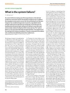
3 Pattern Classification with a Fuzzy System Figure 1 shows the block diagram of the FDI approach proposed in this work. The vectors U (inputs), y (plant outputs), y* (reference outputs) and r (residuals calculated from the observed variables in the different observers)are employed as the input data to a pattern classification system, based on a fuzzy neural network 111. The FDI problem is formulated as a pattern classification. from that data. The pattern classification problem is approached with a learning technique. The And/or newfuzzy topology proposed in [13 is employed. The advantages of this network are: automatic topology definition; knowledgeextraction directly from the database; learning capability; competitive learning without need of derivatives; flexibility in the choice of the 8- and t-norms; fixed processing time and reduced training time for increments in the network dimension; and possibility of rule extraction directly from the network topology. Differently from other works published in the literature, the proposed neurofuzzy network makes the failure detection from both the residuals information and the system operating point information. This allows an increased accuracy in the failure detection procedure. The output block in the diagram of figure 1 is a table which associates each possible pattem to an expression like: "there is afailure in actuator i", or there is a failure that is either in actuatorj or in sensor k ".

5(k f 1) = [I - H(C'H)-LC'] F ( 5 ( k ) , U ( k ) , k ) +

4 Control Reconfiguration Decisor

+H(C'H)-Ly'(k+ 1) + L [C%(k>- y(k)] (5)

in which

means any left inverse of the argument

matrix. 0-7803-7@78-3/0U$l0.00(C)U)ol IEEE

In a situation in which a system failure has been detected, the supervisory system must take some decision Page: 305

Figure 2. DC drive system.

Figure 1. Failure detection and isolation system structure. Note that vector f is employed on28 in the network leaming proceduw.

concerning the c o m e of action after the fault detection. The control reconfiguration will range from a simple change in the observer / controller structure that allows the system continued normal operation,to a sequence of actions that are intended to take the system out of operation safely. The choice of an specific course of action will depend on the nature of the system and of the fault. Independently of the specific situation, there are some abstract actions that can be taken, allowing the system continued control (to its maximum possible extent)after the fault. These actions can be grouped in three sets:

1. restoration of the state variable signal availability 2. restoration of the control signal reliability 3. restoration of system model validity

The actions are strongly related to the sensor failures, the actuator failures, and the system component failures respectively, although the correspondence is not "oneto-one". Action (1) can be directly addressed by a suitable employment of some unknown input observer output. .

The system discrete-time model is:

+ [ 20

"I[$']+[ 0

"fd

[j]=["

e]TL

(8)

"I[]]

0 0 1

lbo observers will be designed. One of them, SM013, is intended to be robust to disturbances in the space directions m and 223, and the other one, SMOa3, to disturbances in the space clirections z2 and xg. Both observers, therefore, will reject the load disturbances, that are injected in direction ZS. Some failure in z1 direction, as a short-circuitin the power source, for instance, would not cause an estimation error in observer SM013. but would do that in observer SMO23. The observer equations are: ~ ~ 0 1 3 :

5 ACaseStudy In this section,the proposed methodology is applied in a DC drive system. The same steps presented here should be followed in the development of a FDI system for any dynamic system to which the methodology is suitable.

The D.C.drive system is composed of two controlled static converters,a D.C.motor and a mechanic load (see figure 2). The considered failures are in the converters, in the motor and in the current and speed sensors. 0-7803-7@78-30l/$l0.00 (C)u)ol IEEE.

[$&[o

1 0 1 o0

] [ y

0 0 1

ar'W = [ art v i

1

(9)

Page: 306

:b1 .................

+

[!

0

q [$]

+

0

[$$I=[

[ ; :][ $: ] [y 0

-Ly'(k)

* ,,

. ... , ..... * I.

1

01 0 1 01

0 0 1 Y'@)

=[

Y?

Yt

I

( 10)

................

The residuals rl and r2 that will be coordinates of the pattern classification procedure are defined a$:

...........

,

In order to study the dynamicalproperties of the residuals after the occurrence of system failures, some simulations of short-circuits and power source turn-off both in the field and in the armature circuits were performed. The reference speed and load torque were randomly generated. In figure 3 the fault occurs at the time 2.5 s. The observer poles were located in [ a1/2 a3 a5/2 ] for observer SMO" and in [ a1 a3/2 a5/2 ] for observer SM023. The choice of the eigenvalues determines the residuals dynamics. A situation of normal operation followed by an m a ture power source turn-off is shown in figure 3. Note that, after the failure occurrence. the residuals r1 and r2 are null, even under the condition of load toque disturbances. Immediately before the failure Occurrence the residual 9-2 varies and r1 stays null, as was expected, since the failure is in direction z1. This fact repeats for the short-circuit in the mature, a failure that is in direction 21 too. When the failures are in ditection x2 (this is the case of short-circuit or turn-off in the field power source) the residual that varies is rl, and r2 stays null.

Ftgure 3. Simulation of normal opemtion followed by an annature power source tum-08. The sequence of events is: t = 0- startup; t = 1.2s- load variation; t = 1.9s- speed reference variation; t = 2.5s- power supply turn-08. The variables in the gmphs are: [top,leftl annature reference current (dashed) and armature current (line); [top,rightj mtor reference speed (dot-dash), rotor speed (dash) and field current (line); [midle,left] residue r1; [midle,right] residue r2; /bottom,lefi] load torque; fiottom,right] failure index. Ezcept the last variable, all the other ones are expressed an P.u..

O

t

The sliding mode observers presented here do not reject measurement disturbances. Therefore, if they exist

they influence the residuals. This can be seen (figure 4 for a failure in the in the field current sensor (that measures variable n).In this case, as output 12 is not being used in observer SMO13, the observed values for it are correct. As the measured values are null, residual rl is affected. These resulLs show that the residuals can be employed for efficient failure detection. However, the residuals values are not enough for the failure classification. Comparing the figures, one can note that the residuals 0-7803-7078-3/0l/$l0.00 (C)u)olIEEE

5

.

.

.

.

.

.

.

.

.

70.

a

5 1

OO

ll.1

Figure 4. DC drive failure simulation: failure in the field c u m n t sensor. Top: residue rl. Bottom: residue 7 2 .

Page: 307

I Fault Index I

Failure description Normal operation

1

I

I

3

I

4

I

5

I

6 7 8

1

Arm. power sourceshort-circuit I

Field power source tum-off Field wwer source short-circuit Armature current sensor failure Field current sensor failure Speed sensor failure

Table 1. DC drive system failures employed in the FDI system simulation.

correct detection and diagnosis

Figure 5. DC drive system structure with remjigumted controi.

faulty sensor by the observed value which is robust to that failure. This means that the output y' that is employed in the controller is replaced by its estimated value.

98.1 %

Table 2. Results of the FDI system in the DC drive system for 1000 faults simulation.

behavior for power source tum-off or short-circuitis almost the same. However, the simulation data shows that it is possible to make the failure classification employing the values of the current and speed meaSurementS in addition to the residuals. For this system, a fuzzy classification engine, imple-

with the A d o r newfuzzy network was employed,with the following parameters:

Inputs:

[

p1 (k)

r2(k) pl (k) p2(k) vs (k)

3

0

Number of fuzzy partitions for each input: 3

0

Number of outputs: 8 (classes, failure index, table 1)

In order to test the failure detection system, a set of 2000 failure simulations was created, with randomly generated index. The first lo00 simulations were employed for the neural network learning procedure, and the last lo00 one.. were used as a validation set. The simulations were performed with load disturbance, speed reference, time of occurrence and value randomly generated. The result is presented in table 2.

The field and armature currents and the speed are controlled variables of the DC servo-system. Therefore, sensor failures can cause significant errors between the reference and the real values. In order to illustrate, figure 6 (top) shows the speed and speed reference behavior for a normal operation (with the motor in twice the nominal speed), followed by a failure in the field current sensor in t = 2.5s. As the field Current is measured as null (less than the reference), the control acts in order to reduce the error, increasing the field voltage. This leads to an increment in the field current (figure 5, bottom) and in the field flux. This flux increment causes a sped reduction. The speed will stabilize in a value that is different from its reference, with significant error. The procedure proposed here is: once the sensor fault is detected, the measured value is replaced by the observed vdue that is correct. In this case, the output of S M O ' ~ is robust to this fault, preserving the correct value of the variable. Figure 7 shows the same simulation, employing this reconfiguration scheme. In this case, the field current sensor failure was detected after 0.1 seconds. Note that after the observed value is introduced in the convol loop, replacing the wrong measured value, the system returns to a null speed error. Due to the large mechanical time constant, the speed is disturbed to a small amount during the 0.1 s before the failure detection.

6 5.1 Control Reconfiguration for Sensor Failure In this item, an application of the failuredetection strategy in control reconfiguration is presented (figure 5). The basic idea is to replace the measured value in the 0-7803-7@78-3/Ol/$lO.~ (C)u)ol LEEE.

Conclusion

The failure detection structurepresented here, based on sliding mode observers, is more robust to plant parameter variations and model uncertainties than the known structures. based on classical observers. This robust behavior seems to be similar to the behavior of other FDI

Page: 308

strategies [3, 41 that are based on unknown input observers too. 2.5

I

I

1

0'2

0'3

04

0'5

0'8

0'7

08

09

1 [*I

or

01

02

03

04

016

01

0'7

0.8

!

0'9

I [SI

Figure 6. Simulation of a failure in the field current sensor for the system without r e m figuration. Top: reference rotor speed (dash) and rotor speed (line). Bottom: reference field current (dash), field current (dot-dash) and measuredfield current (line). All variables are ezpressed in p-U.

!

An advantage of the sliding mode approach, proposed here, is the simplicity of the observer design which, in the case of the DC drive, could be performed algebraically. The application of this failure detection strategy as a tool for control system reconfiguration in the caqe of sensor failure ha5 been shown to be a viable alternative. In addition to this, the employment of the pattern recognition system for residuals processing allows the automaticgeneration of the decision logic. Note that this task is not trivial [2].

The decision logic obtained from the pattern recognition system leads to a more robust FDI system than the methods based on residual threshold detection. This superiority comes from the additional information that is employed in the first case: the plant operating point (which is associated to the plant inputs and outputs).

References W. M. Caminhas, H. M. F. Tavares, E Gomide, and W.Pedrycz. Fuzzy set based neural networks: structure, leaning and application. J. Advanced Computational lntelligence, 3(3):151-157, 1999. P. M. Frank. Fault Diagnosis in Dynamic Systems Using Analytical and Knowledge-based redundancy - A Survey and Some New Results. Awomatica, 26(3):459474, 1990. P. M. Frank and I. Wiinnenberg. Robust fault diagnosis using unknown input observer schemes. In R. J. Patton, P. M. Frank, and R. N.Clark,editors, Faulr Diagnosis in Dynamic Sysrms: Theory and Applications, pages 4798.Prentice-Hall, 1989. W.Ge and C. Z. Fang. Detection of Faulty Components Via Robust Observation. Int. J. Control, 47581-599, 1988. R. Isermann and D. Fiissel. Supervision, fault-detection and faultdiagnosis methods. In H. Zimmermann, editor, Practical Applications of Fuuy Technologies, pages 119159. Kluwer Academic Publishers, 1999. R. I. Patton, P. M. Frank, and R. N. Clark Fault Diagnosis in Dynamic Sysrems: Theory and Applicatiom. Prentice-Hall, 1989. R. H. C. Takahashi and P. L. D. P a s . Unknown input observers: a unifying approach. European Journal of Conrml, 5(2):261-275, 1999.

Figure 7. Simulation of a failure in the field current sensor for the system with reconfigumtion. Top: refewnce rotor speed (dash) and rotor speed (line). Bottom: reference field current (dash), field cumnt (dot-dash) and measured field current (he). All variables are eapressed in p.U.

0-7803-7078-3/0U$10.00 (C)u)ol IEEE

Page: 309