Neural Networks architectures for modelling dynamic signals and systems ...
Chapters 4, 5 and 6 from [Haykin, 1994] S. Haykin Neural Networks – A ...
1
Lecture 11: Adaptive Nonlinear Filters Neural Networks Overview • Linear Perceptron Training ≡ LMS algorithm • Perceptron algorithm for Hard limiter Perceptrons • Delta Rule training algorithm for Sigmoidal Perceptrons • Generalized Delta Rule (Backpropagation) Algorithm for multilayer perceptrons • Training static Multilayer Perceptron • Temporal processing with NN – Neural Networks architectures for modelling dynamic signals and systems – Reduction of dynamic NN to static NN training through unfolding References: Chapters 4, 5 and 6 from [Haykin, 1994] S. Haykin Neural Networks – A comprehensive foundation Macmillan College Publishing Company, 1994.
Lecture 11
Linear Perceptron
• A linear combiner has N inputs and one output. • An FIR filter of order N is similar, but its N inputs are all shifted-in-time versions of the same signal.
2
3
Lecture 11
Linear Perceptron Training ≡ LMS algorithm LMS algorithm for a linear FIR filter (REMINDER) Given
• the (correlated) input signal samples {u(1), u(2), u(3), . . .}, generated randomly; • the desired signal samples {d(1), d(2), d(3), . . .} correlated with {u(1), u(2), u(3), . . .}
1 Initialize the algorithm with an arbitrary parameter vector w(0), for example w(0) = 0. 2 Iterate for t = 0, 1, 2, 3, . . . , nmax 2.0 Read a new data pair, (u(t), d(t)) P −1 2.1 (Compute the output) y(t) = w(t)T u(t) = M i=0 wi (t)u(t − i) 2.2 (Compute the error) e(t) = d(t) − y(t) 2.3 (Parameter adaptation) w(t + 1) = w(t) + µu(t)e(t) u(t) w (t + 1) w (t) 0 0 w1 (t) w1 (t + 1) u(t − 1) . . . = + µe(t) or componentwise . . . . . . u(t − M + 1) wM −1(t + 1) wM −1(t) 2
4
Lecture 11
LMS algorithm derivation for Linear Combiner (Review) The Linear Combiner (linear neuron, or linear perceptron) has N inputs, which can be grouped into the vector h iT u(t) = u1(t) u2 (t) . . . uN (t) has also N parameters or weights (synaptic strength) h
w = w1 w2 . . . wN and computes its output as
y(t) = wT u(t) =
N X
iT
wiui (t)
i=1
which probably is not equal to the desired signal d(t), the error being e(t) = d(t) − y(t) = d(t) − wT u(t) The performance criterion is J(w) = E[e2(t)] = E[(d(t) − y(t))2] = E[(d(t) − wT u(t))2] and must be minimized with respect to w. At the minimum, the gradient vector must be zero ∇w J(w) = 0 ∇w J(w) = ∇w E[e2(t)] = 2Ee(t)∇w [(e(t)] = 2Ee(t)∇w [(d(t) − wT u(t))] = −2Ee(t)u(t) = 0 The gradient method for minimizing the criterion E[e2(t)] requires the modification at each time step of the parameter vector with a small step in the reversed direction of gradient vector: 1 w(t + 1) = w(t) − µ∇w(t) J(w(t)) = w(t) + µ[Ee(t)u(t)] 2
5
Lecture 11
In order to simplify the algorithm, instead the true gradient of the criterion ∇w(t) J(t) = −2Eu(t)e(t) LMS algorithm will use an immediately available approximation ˆ w(t) J(t) = −2u(t)e(t) ∇ Using the noisy gradient, the adaptation will carry on the equation 1 ˆ w(t + 1) = w(t) − µ∇ w(t) J(t) = w(t) + µu(t)e(t) 2
Lecture 11
A Reminder of the circuit implementing the LMS algorithm
6
Lecture 11
7
A similar circuit implementing the adaptation of the linear combiner (perceptron)
8
Lecture 11
LMS algorithm for a Linear Combiner Given
• the (correlated) input vector samples {u(1), u(2), u(3), . . .}, generated randomly; • the desired signal samples {d(1), d(2), d(3), . . .}
1 Initialize the algorithm with an arbitrary parameter vector w(0), for example w(0) = 0. 2 Iterate for t = 0, 1, 2, 3, . . . , nmax 2.0 Read a new data pair, (u(t), d(t)) P 2.1 (Compute the output) y(t) = w(t)T u(t) = N i=1 wi (t)ui (t) 2.2 (Compute the error) e(t) = d(t) − y(t) 2.3 (Parameter adaptation) w(t + 1) = w(t) + µu(t)e(t) w (t + 1) w (t) u (t) 1 1 1 u2 (t) w2 (t + 1) w2 (t) . . . or componentwise = + µe(t) . . . . . . uN (t) wN (t) wN (t + 1) 2
Lecture 11
9
A Redrawing of the circuit implementing the adaptation of the linear combiner (perceptron)
Lecture 11
Generalizing the linear combiner to a layer of M linear combiners
10
11
Lecture 11
Perceptrons with Hard Nonlinearities A perceptron with hard nonlinearity (the proper perceptron) is a linear combiner followed by one “hard” nonlinearity h = h[0,1] or h = h[−1,1] y(t) = h[wT u(t)] = h0,1 [
N X
wiui (t)]
i=1
where [0,1]
h
[−1,1]
h
(x) =
1, x ≥ 0 0, x < 0
(x) = sign(x) =
1, x ≥ 0 −1, x < 0
Defining as before the error e(t) = d(t) − y(t) the performance criterion can be written as either MSE (mean square error) or MAE(mean absolute error) J(w) = E[e2(t)] = E[(d(t) − y(t))2] = E[|e(t)|] (for binary values of d(t) and y(t) MSE and MAE are identical), and must be minimized with respect to w. The gradient is ∇w J(w) = ∇w E[e2 (t)] = 2Ee(t)∇w [(e(t)] = 2Ee(t)∇w (d(t) − h[wT u(t)]) = −2Ee(t)u(t)h′ [wT u(t)]
12
Lecture 11
The problem with this expression is that almost everywhere h′ = 0 so the gradient based updating will be zero almost all the time, and when it is not zero, the derivative is not defined. However, using an algorithm with the updating w(t + 1) = w(t) + u(t)e(t) will result in a powerful result:
If there is a vector w 0 which makes the criterion zero, the algorithm will find in a finite number of iterations a parameter vector making the criterion zero (probably not w0, since in general there are many different parameter vectors for which the criterion is zero).
13
Lecture 11
Perceptron algorithm Given
• the (correlated) input vector samples {u(1), u(2), u(3), . . .}, generated randomly; • the desired signal samples {d(1), d(2), d(3), . . .}
1 Initialize the algorithm with an arbitrary parameter vector w(0), for example w(0) = 0. 2 Iterate for t = 0, 1, 2, 3, . . . , nmax 2.0 Read a new data pair, (u(t), d(t)) P 2.1 (Compute the output) y(t) = sign[w(t)T u(t)] = sign[ N i=1 wi (t)ui(t)] 2.2 (Compute the error) e(t) = d(t) − y(t) 2.3 (Parameter adaptation) w(t + 1) = w(t) + u(t)e(t) w (t + 1) w (t) u (t) 1 1 1 u2 (t) w2 (t + 1) w2 (t) . . . or componentwise = + e(t) . . . . . . uN (t) wN (t) wN (t + 1) 2
Lecture 11
14
A circuit implementing the adaptation of the perceptron with hard nonlinearity
15
Lecture 11
Perceptrons with Sigmoidal Nonlinearities A perceptron with a sigmoidal nonlinearity is a linear combiner followed by a monotonically increasing nonlinearity h y(t) = h[wT u(t)] where, e.g. h can be the nonsymmetrical function h(x) =
1 1 + e−βx
or the symmetrical function 1 − e−βx h(x) = 1 + e−βx Now the derivation we tried for the hardlimiter nonlinearity will be meaningful: The gradient ∇w J(w) = ∇w E[e2 (t)] = 2Ee(t)∇w [(e(t)] = 2Ee(t)∇w (d(t) − h[wT u(t)]) = −2Ee(t)u(t)h′ [wT u(t)] can be approximated by ∇w J(w) ≈ −2e(t)u(t)h′ [wT u(t)] and then use the gradient based update w(t + 1) = w(t) + µu(t)e(t)h′[wT (t)u(t)] The computation of the derivative can be done using (for the nonsymmetrical sigmoid) h′ [x] = h(x)(1 − h(x))
16
Lecture 11
Delta Rule Algorithm Given
• the (correlated) input vector samples {u(1), u(2), u(3), . . .}, generated randomely; • the desired signal samples {d(1), d(2), d(3), . . .}
1 Initialize the algorithm with an arbitrary parameter vector w(0), for example w(0) = 0. 2 Iterate for t = 0, 1, 2, 3, . . . , nmax 2.0 Read a new data pair, (u(t), d(t)) P 2.1 (Compute the output) y(t) = h[w(t)T u(t)] = h[ N i=1 wi (t)ui(t)] 2.2 (Compute the error) e(t) = d(t) − y(t) ′ T 2.3 (Parameter adaptation) w(t + 1) = w(t) + µu(t)e(t)h [w (t)u(t)] w (t + 1) w (t) u1(t) 1 1 w2 (t + 1) w2 (t) u2 (t) . . . ′ T or componentwise = + µe(t)h [w (t)u(t)] . . . . . . wN (t) wN (t + 1) uN (t) 2
Lecture 11
17
A circuit implementing the adaptation of the perceptron with sigmoidal (soft) nonlinearity
18
Lecture 11
Multilayer Perceptrons 1. Multilayer Perceptron: Consider a three layers perceptron (having two hidden layers). The first perceptron layer has �
• n1 inputs, u[1] = u[1] . . . u[1] 1 n1
�T
and n2 neurons;
• The weight matrix W[1] with dimensions n2 × n1 ; • the activations v • the outputs u
[2]
[1]
=
�
[1] v1
�
= u[2] 1
. . . vn[1]2 �T [2] . . . u n2
�T
of the neurons are computed as v [1] = W[1] u[1]
of the neurons are computed as u[2] = h(v [1] )
2. The second perceptron layer has • n2 inputs, u
[2]
=
�
[2] u1
...
u[2] n2
�T
and n3 neurons;
• The weight matrix W[2] with dimensions n3 × n2 ; �
• the activations v [2] = v1[2] . . . vn[2]3 • the outputs u
[3]
=
�
[3] u1
...
u[3] n3
�T
�T
of the neurons are computed as v [2] = W[2] u[2]
of the neurons are computed as u[3] = h(v [2] )
3. The third perceptron layer has • n3 inputs, u
[3]
=
�
[3] u1
...
u[3] n3
�T
and n4 neurons;
• The weight matrix W[3] with dimensions n4 × n3 ;
19
Lecture 11
• the activations v
[3]
=
�
• the outputs y = u[4] =
�T [3] [3] of the neurons are computed as v [3] = W[3] u[3] v 1 . . . v n2 � �T [3] [3] of the neurons are computed as y = u[4] = h(v [3]) u 1 . . . u n4
The computation of the output y with the multilayer perceptron is realized using v [1] = W[1] u[1] ; v [2] = W[2] u[2] ; v [3] = W[3] u[3] ;
u[2] = h(v [1] ) u[3] = h(v [2] ) y = u[4] = h(v[3] )
or written componentwise [1]
vi = [2]
vi = [3]
vi =
n1 X
j=1 n2 X j=1 n3 X j=1
[1] [1]
ui = h(vi )
[2] [2]
ui = h(vi )
[3] [3]
yi = ui = h(vi )
wij uj wij uj wij uj
[2]
[1]
i = 1, . . . , n2
[3]
[2]
i = 1, . . . , n3
[4]
[3]
i = 1, . . . , n4
Lecture 11
A circuit implementing the multilayer perceptron
20
21
Lecture 11
The optimality criterion can be selected to take into account the norm of errors at time t: n4 n4 1X 1X 1 [4] 2 Jt = (di(t) − ui (t)) = e2 (t) = eT e 2 i=1 2 i=1 2
(1)
Another choice is to evaluate with the criterion the overall training set (t = 1, . . . , Nset) performance of the neural network set 1 NX J= Jt (2) 2 t=1 In order to minimize (1) and (2) we introduce some notations, and derive the BP algorithm: ∂Jt [3] ∂vi
[4]
∂Jt ∂ui
=
[4] ∂ui
[3] ∂vi
[4]
[3]
∆ = −(di − ui )h′(v [3] ) = −δi
(3)
For the output layer the gradient computation is straightforward ∂Jt [3] ∂wij
[3]
∂Jt ∂vi
=
[3] [3] ∂vi ∂wij
[3] [3]
= −δi uj
(4)
For any hidden layer, we recognize that [k+1]
∂vi
[k] ∂vj
[k+1]
=
∂vi
[k] ∂uj
[k]
∂uj
[k] ∂vj
[k]
[k]
= wij h′ (vj )
(5)
and ∂vn[k+1] [k]
∂wij
[k]
= uj , n = i 0, n 6= i
(6)
22
Lecture 11
Now we can apply the rule for derivative of a compose function ∂Jt [k] ∂vj
=
nX k+2
[k+1]
∂Jt ∂vi
[k+1] i=1 ∂vi
∂Jt [k] ∂wij
=
[k] ∂vj
nX k+1
=
nX k+2 [k] [k] [k] ∆ − δi wij h′ (vj ) = i=1
∂Jt ∂vp[k+1]
[k+1] p=1 ∂vp
[k] ∂wij
[k] [k]
= −δi uj
[k−1]
−δj
(7)
(8)
23
Lecture 11
Backpropagation Algorithm 1. Initialization of weight matrices,W[1] (1), W[2](1), W[3] (1) at time instant t = 1 with small random numbers. 2. For it = 1, 2, 3, . . . , Nit 2.0 Initialize
∂J(it) [k] ∂wij
!
← 0, k = 1, 3, j = 1, nk , i = 1, nk+1, J(it) ← 0
2.1 For n = 1, 2, . . . , Nset (we omit writing the time argument (t)) 2.1.0 Read a new element (u[1] (t), d(t))) 2.1.1 Forward computations ”FORWARD PATH” v [1] = W[1] u[1] , u[2] = h(v [1] ) u[3] = h(v [2] ) v [2] = W[2] u[2] , v [3] = W[3] u[3] , u[4] = h(v [3] ) e = d(t) − u[4] ,
Jt = eT e =
n4 X
e2j
j=1
J(it) ← J(it) + Jt
24
Lecture 11
2.1.2 Backward computation ”BACKWARD PATH”
Compute the generalized errors for all neurons, starting with last layer [3]
[4]
[3]
δi = (di(t) − ui )h′ (vi ) [2]
[2] Pn4 [3] [3] j=1 wji δi [1] P 3 [2] [2] h′ (vi ) nj=1 wji δi
δi = h′ (vi ) [1]
δi =
i = 1, n4 i = 1, n3 i = 1, n2
Compute the elements of the gradients, ∂Jt [1] ∂wij
!
= −uj δi
∂Jt [2] ∂wij
!
= −uj δi
∂Jt [3] ∂wij
!
= −uj δi
[1] [1]
i = 1, n2, j = 1, n1
[2] [2]
i = 1, n3, j = 1, n2
[3] [3]
i = 1, n4, j = 1, n3
∂Jt [1] ∂wij
2.1.3 Accumulate the gradient elements J(it) ∂J(it) [k] ∂wij
!
←
∂J(it) [k] ∂wij
!
+
∂Jt [k] ∂wij
!
, k = 1, 3, j = 1, nk , i = 1, nk+1
2.2 If J(it) < ε STOP 2.3 Modify the wheight values in !the direction opposed to gradient vector [1]
[1]
[2]
[2]
[3]
[3]
wij (it + 1) = wij (it) − λ
wij (it + 1) = wij (it) − λ wij (it + 1) = wij (it) − λ
∂J [1] ∂wij it ! ∂J [2] ∂wij it ! ∂J [3] ∂wij it
25
Lecture 11
y1 = u41 y2 = u42 yn4 = u4n4 6
6
h v13
h
6
v23
6
e1 = d1 − y1 en4 = dn4 − yn4
6
h 3 vn4
3
3 3
6u3 6 2
u3n3
6
-
′
h h′
v =W u u31
h v12
h
6
v22
6
W δ
6
-
h′ h′
v2 = W2 u2 u21
6u2 6 2
h v11
u2n2
h
6
v21
6
W δ
1 vn2
6
-
u11
6
u12
′
h h′
? � -× � δ1 ? 1
? � -× 1 � δn2 ?
δ 1 u1T 6
v =W u 6
-
6
∂J − ∂W 2
u21 u2n2
6
1 1
1
? � -× ? � 2 � δ -× n3 2 2T � δ2 - δ u ? 1 ? 6 6 2T 2
h
∂J − ∂W 3
u31 u3n3
6
h 2 vn3
? � -× ? � 3 � δ -× n4 3 3T � δ13 - δ u ? ? 6 6 3T 3
6
u11 u1n1
u1n1
Figure 1: Circuit implementing Backpropagation algorithm
∂J − ∂W 1
Lecture 11
26
Temporal processing with Neural Networks Neural Networks architectures for modelling dynamic signals and systems • NN with linear dinamic synapses: FIR multilayer perceptron and Time Delay Neural Networks • Mixed NN – Transfer function model • Standard nonlinear state space models
Generalization of static NN models to dynamic NN models • Definition 1: A static NN is characterized by : – has memoryless transmitance of the synapse, wij , between the output of neuron j and the input of neuron i; – there are no feedback loops (once there is a connection from neuron i to neuron j, there is no connection path from neuron j back to neuron i. • Definition 2: A dynamic NN satisfies one of the following conditions: – either has a nontrivial transfer function at some synapses (a linear filter) wij (q −1), between the output of neuron j and the input of neuron i (e.g. FIR multilayer perceptrons). – or it contains feedback loops: dynamic feedback loops (not algebraic loops) (e.g. reccurent neural networks). – or it is formed by composing Linear Filters structures with Neural Network structures (not necessarily at synapse level).
27
Lecture 11
NN with linear dinamic synapses: FIR multilayer perceptrons The basic model of a neuron can be generalized to include memory elements, (like delay elements). Consider the classical sigmoidal perceptron, which processes the inputs u1, u2, . . . , uN as v =
N X
wi u i = w T u
i=1
y = h(v) to obtain the output y. We don’t specify the time moment t since all variables have the same time argument. The nonlinear function h(·) can be either symmetric sigmoid or the asymmetrical sigmoid. A dynamic neuron can be defined as v(t) =
N X
wi(q −1)ui(t)
i=1
y(t) = h(v(t)) where each wi(q −1) is a FIR filter.
Lecture 11
Static and dynamic neurons
28
29
Lecture 11
A FIR multilayer perceptron is obtained replacing all neurons in a multilayer perceptron by dynamic neurons.
Example For notation simplicity, consider dynamic neurons FIR filters of order 3. Consider a three layers perceptron (having two hidden layers). We define for the first perceptron layer (for other layers notations are straightforward extensions of static multilayer perceptron) [1]
• n1 inputs, u
=
�
[1] u1
...
u[1] n1
�T
and n2 neurons;
• The matrix of transfer functions W[1] (q −1) with n2 × n1 elements, [1]
[1]
[1]
W[1] (q −1) = w0 + w1 q −1 + w2 q −2 [1]
[1]
[1]
where the matrices w0 , w1 , and w2 have dimensions n2 × n1; • the activations v
[1]
=
�
[1] v1
...
vn[1]2
�T
of the neurons are computed as [1]
[1]
[1]
v [1](t) = W[1] (q −1)u[1] (t) = w0 u[1] (t) + w1 u[1] (t − 1) + w2 u[1] (t − 2) or elementwise [1]
vi (t) =
n1 X
j=1
[1]
[1]
Wij (q −1)uj (t) =
n1 X
[1]
[1]
[1]
[1]
[1]
[1]
(w0ij uj (t) + w1ij uj (t − 1) + w2ij uj (t − 2))
j=1
30
Lecture 11
[2]
• the outputs u
=
�
[2] u1
...
u[2] n2
�T
of the neurons are computed as u[2] (t) = h(v [1](t))
The resulting FIR multilayer perceptron is shown in Figure (a).
Lecture 11
A circuit implementing the adaptation of the FIR multilayer perceptron
31
32
Lecture 11
Reduction of dynamic NN training to static NN training through unfolding The optimality criterion can be selected to take into account the norm of errors at time t: n4 n4 1X 1 1X 1 T 2 Jt = (di(t) − yi (t)) = (d(t) − y(t)) (d(t) − y(t)) = e2 (t) = e(t)T e(t) 2 i=1 2 2 i=1 2
(9)
Another choice is to evaluate with the criterion the overall training set (t = 1, . . . , Nset) performance of the neural network set 1 NX J= Jt (10) 2 t=1 [1]
The derivative of criterion Jt with respect to an elemental weight, say, w0ij , of the FIRMP can be computed applying the derivative chain rule to the system of equations [1] vi (t)
=
n1 X
[1]
[1]
[1]
[1]
[1]
[1]
i = 1, . . . , n2, j = 1, . . . , n1
[2]
[2]
i = 1, . . . , n3, j = 1, . . . , n2
[3]
[3]
i = 1, . . . , n4, j = 1, . . . , n3
(w0ij uj (t) + w1ij uj (t − 1) + w2ij uj (t − 2)),
j=1 [2]
[1]
ui (t) = h(vi (t)), [2]
vi (t) =
n2 X
[2]
i = 1, . . . , n2,
[2]
[2]
[2]
(w0ij uj (t) + w1ij uj (t − 1) + w2ij uj (t − 2)),
j=1 [3]
[2]
ui (t) = h(vi (t)), [3]
vi (t) = yi (t) = Jt =
n3 X
[3]
i = 1, . . . , n3,
[3]
[3]
[3]
(w0ij uj (t) + w1ij uj (t − 1) + w2ij uj (t − 2)),
j=1 [4] ui (t) n4 X
[3]
= h(vi (t)),
(di(t) − yi (t))2
i=1
i = 1, . . . , n4,
33
Lecture 11
Once the gradients dJt [k]
dwlij
for all defined k, l, i, j are computed, the updating of the weights will take place as: [k]
[k]
wlij (t + 1) = wlij (t) − µ
dJt [k]
dwlij
Unfolding the FIR MP One equivalent way to perform the training of FIR MP is to use the standard Backpropagation algorithm for an unfolded structure, as in Figure (b). • Establish the structure of the static multilayer perceptron,(number of neurons in each layer) ex In the first layer: (15 × n1 × n2 ) nonzero weights, there are nex 1 = 15n1 inputs and n2 = 5n2 outputs; ex In the second layer: (9 × n2 × n3 ) nonzero weights, there are nex 2 = 5n2 inputs and n3 = 3n3 outputs; ex In the third layer: (3 × n3 × n4 ) nonzero weights, there are nex 3 = 3n3 inputs and n4 = n4 outputs.
• In the connection matrices W[ex1] , W[ex2], W[ex3] , many weights are constraint to zero; • Some other weights must obey equality constraints (e.g. in the first layer connections matrix W[ex1] , the [1] block W0 appears five times). • Apply one step of BP algorithm to the MP W[ex1] , W[ex2] , W[ex3] , finding the gradients with respects to all nonzero weights in the matrices W[ex1] , W[ex2] , W[ex3] .
Lecture 11
34
• Find the constraint gradients, with respect to original FIR MP weights, by adding all corresponding gradients in MP. • change the weights using the constraint gradients. • iterate until convergence.