Army Belvoir R D & E Center under contract #DAAK70-92-K-. 0003. Note that this model is equally applicable for both scalar and vector sequences. The use of ...
MODELING NONLINEAR DYNAMICS WITH NEURAL NETWORKS: EXAMPLES IN TIME SERIES PREDICTION Eric A. Wan
Stanford University, Department of Electrical Engineering, Stanford, CA 94305-4055 �
Abstract| A neural network architecture is discussed which uses Finite Impulse Response (FIR) linear lters to provide dynamic interconnectivity between processing units. The network is applied to a variety of chaotic time series prediction tasks. Phase-space plots of the network dynamics are given to illustrate the reconstruction of underlying chaotic attractors. An example taken from the Santa Fe Institute Time Series Prediction Competition is also presented. I. Introduction
The goal of time series prediction can be stated succinctly as follows: given a nite sequence y(1); y(2); : : : y(N ), nd the continuation y(N + 1); y(N + 2)::: The series may arise from the sampling of a continuous time system, and be either stochastic or deterministic in origin. Applications of prediction range from modeling turbulence to di�erential pulse code modulation schemes for telecommunication to stockmarket portfolio management. The standard prediction approach involves constructing an underlying model which gives rise to the observed sequence. In the oldest and most studied method, a linear autoregression (AR) is t to the dqata: y(k) =
X ( ) ( ? ) + ( ) = ^( ) + ( ) T
n=1
anyk
n
ek
yk
ek:
(1)
This AR model forms y(k) as a weighted sum of past values of the sequence. The single step prediction for y(k) is given by y^(k). Neural networks may be used to extend the linear model to form a nonlinear prediction scheme. The basic form y(k) = y^(k) + e(k) is retained; however, the estimate y^(k) is taken as the output N of a neural network driven by past values of the sequence: y(k) = N [y(k ? 1); y(k ? 2); :::y(k ? T )] + e(k): (2)
� We wish to acknowledge the support of NSF under grant NSF IRI 91-12531, of ONR under contract no N00014-92-J-1787, of EPRI under contract RP:8010-13, and of the Department of the Army Belvoir R D & E Center under contract #DAAK70-92-K0003.
Note that this model is equally applicable for both scalar and vector sequences. The use of this nonlinear autoregression can be motivated as follows. First, Takens Theorem (Takens 1981) implies that for a wide class of deterministic systems there exists a di�eomorphism (one-to-one di�erential mapping) between a nite window of the time series [y(k ? 1); y(k ? 2); :::y(k ? T )] and the underlying state of the dynamics system which gives rise to the time series. This implies that there exists, in theory, a nonlinear autoregression of the form y(k) = g[y(k ? 1); y(k ? 2); :::y(k ? T )], which models the series exactly (assuming no noise). The neural network thus forms an approximation to the ideal function g(�). Furthermore, it has been shown (Hornik et al. 1989; Cybenko 1989; Irie and Miyake 1988) that a feedforward neural network N with an arbitrary number of neurons and 2 or more layers is capable of approximating any uniformly continuous function. These arguments provide the basic motivation for the use of neural networks in time series prediction. II. Network Architecture and Prediction Configuration
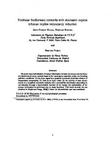
The use of neural networks for time series prediction is not new. Previous work includes (Werbos 1974, 1980; Lapedes and Farber 1987; Weigend et al. 1990) to cite just a few. In this paper, we focus on a method for achieving the nonlinear autoregression by use of a Finite Impulse Response (FIR) network (Wan 1990, 1993. The network resembles a standard feedforward network where each synapse is replaced with an adaptive FIR linear lter as illustrated in Fig. 1. The FIR lter forms a weighted sum of past values of its input. The neuron receives the ltered inputs and then passes the sum through a nonlinear squashing functions. Neurons are arranged in layers to form a network in which all connections are made with the synaptic lters. Training the network is accomplished through a modi cation of the backpropagation algorithm (Rumelhart et al. 1986) called temporal backpropagation in which error terms are symmetrically ltered backward through the network. A complete description of the architecture along with the
x(k)
q-1
w(0)
x(k-1)
x(k-2)
q-1
q-1
w(2)
w(1)
x(k-T)
Training:
w(T) y(k)
^ y(k)
y(k-1)
e(k)
+
x1l-1 (k) l-1
x2 (k)
FIR filters
q-1
w l1j
y(k)
w l2j
+
xjl (k)
w l3j
x3l-1 (k)
Neuron
Prediction: ^y(k-1)
^y(k)
1.0
q-1
Fig. 2: Network prediction con guration: (a) Training. (b) Iterated prediction.
This closed-loop system is illustrated in Fig. 2b. The system can be iterated forward in time to achieve predictions as far into the future as desired. III. Examples of chaos prediction and attractor reconstruction
Fig. 1: FIR network architecture (q?1 represents a time-domain unit delay operator)
In the examples that follow, networks of various dimensions are trained on time series generated by chaotic processes. The long term iterated prediction of the networks are then analyzed.
training algorithm can be found in (Wan 1993).
A. Results of the SFI Competition
Fig. 2a illustrates the basic predictor training con guration. At each time step, the input to the FIR network is the known value y(k ? 1), and the output y^(k) = Nq [y(k ? 1)] is the single step estimate of the true series value y(k). Our model construct is thus: y(k) = Nq [y(k ? 1)] + e(k): Since the FIR network has only a nite memory of past samples, Nq [y(k ? 1)] is equivalent to a nite nonlinear regression on y(k). During training, the squared error e(k)2 = (y(k) ? y^(k))2 is minimized by using the temporal backpropagation algorithm to adapt the network. Note we are performing open-loop adaptation; both the input and desired response are provided from the known training series. Once the network is trained, long-term iterated prediction is achieved by taking the estimate y^(k) and feeding it back as input to the network: y^(k) = Nq [^y (k ? 1)].
Chaotic intensity pulsations in a single-mode far infrared NH3 laser
250
200
Intensity
Network
150
100
50
0
200
400
600
800
1000
k
Fig. 3: 1000 points of laser data.
During the fall of 1991, The Santa Fe Institute Time
were not provided and were not available when the predictions were submitted. As can be seen, the prediction is remarkably accurate with only a slight eventual phase degradation. A prediction based on a 25th order linear autoregression is also shown to emphasize the di�erences from traditional linear methods. Other submissions to the competition included methods of k-d trees, piecewise linear interpolation, low-pass embedding, SVD, nearest neighbors, Wiener lters, as well as standard recurrent and feedforward neural networks. As reported by the Santa Fe Institute, the FIR network outperformed all other methods on this data set.
Iterated Network Prediction
250
200
150
100
50
0
1020
1040
1060
1080
1100
k
B. Mackey-Glass Mackey-Glass(30) Time Series
Best Linear Predictor 1.4 250 1.2 200
1
x
0.8 150
0.6 100 0.4 50
0
0.2 0 0 1020
1040
1060
1080
100
200
300 k
1100
400
500
600
k
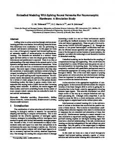
Fig. 4: (a) Network prediction (solid line) and series continuation (dashed line). (b) linear AR prediction.
Mackey-Glass(30) Iterated Prediction 1.4
Series Prediction and Analysis Competition was estab-
The 100 step prediction achieved by using an FIR network (dimensions: 1x12x12x1 neurons with 25:5:5 order lters) is shown in Fig. 4 along with the actual series continuation for comparison. It is important to emphasize that this prediction was made based on only the past 1000 samples. True values of the series for time past 1000 � \Measurements were made on an 81.5-micron14NH3 cw (FIR) laser, pumped optically by the P(13) line of an N20 laser via the vibrational aQ(8,7) NH3 transition" - (Huebner 1989).
1 0.8 x
lished as a means for evaluating and benchmarking new and existing techniques in time series prediction (Weigend and Gershenfeld 1993). The plot in Fig. 3 shows the chaotic intensity pulsations of an N H3 laser � distributed as part of the competition. Contestants were given only 1000 points of data and then invited to send in solutions predicting the next 100 points. During the course of the competition, the physical background of the data set, as well as the 100 point continuation, was withheld to avoid biasing the nal prediction results.
1.2
0.6 0.4 0.2 0
520
540
560
580
600
k
Fig. 5: (a) Mackey-Glass(30) delay-di�erential equation. (b) Iterated prediction (solid line) and series continuation (dashed-line).
For the next example we consider the Mackey-Glass delay-di�erential equation (Glass 1977): �) : dx(t) = ?0:1x(t) + 1 0+:2xx((tt?? �) (3) 10 dt with parameters � = 17 and 30, initial conditions x(t) = 0:9 for 0 � t � �, and sampling rate � = 6. These
Henon Map 0.4 0.3 0.2 0.1
x(k-1)
Table 1: Comparison of log normalized single step prediction errors for Mackey-Glass (small numbers mean a better prediction). Linear Poly. Rational loc(1) MG(17) -0.57 -1.95 -1.14 -1.48 MG(30) -0.49 -1.40 -1.33 -1.24 loc(2) RBF N.Net FIR Net MG(17) -1.89 -1.97 -2.00 -2.31 MG(30) -1.42 -1.60 -1.50 -1.79
0 -0.1 -0.2 -0.3
parameters were chosen to facilitate comparisons with prior work (Farmer and Sidorowich 1987; Lapedes and Farber 1987; Casdagli 1989). The time series for � = 30 is shown in Fig 5a. An FIR network with 1 � 15 � 1 nodes and 8 : 2 in taps in each layer was trained on only the rst 500 points of the series. The resulting log normalized single step prediction errors for the subsequent 1500 points are given in Table 1 along with results of other methods as summarized in (Casdagli 1989). While the FIR network shows a slight improvement over existing methods, the single step prediction task is really not that di�cult. A more challenging problem is the iterated prediction as shown in Fig. 5b. The network receives no new inputs past the point 500. The iterated 100 point prediction is remarkably accurate. C. H�enon Map
-0.4 -1.5
.................................... .......................................... ..................................... . ................ ....................... .................. ................... ............... ..................... ... ............... ............... . .................................... ............... .............. ................................ ............ .................. ............ ............ ...................................................... ......... ........ ............................ .......... ....... ............................................. ........... ............... ...................................... . .......... ................ ............................. .. ............... ........ .............. ........ ............. ............................................................ ....... ............ .............................. ....... ............ ............................ ....... ........... .......................... ...... ........... ..................... ..................... ..... .......... ................. .... ....... .... ....... ................... ................. ... .. ... .. ............... .......... ... ... ... ... ... ... ... .. . . . . ... ... ..... ..... .. .. ..... .... .. ... .. ..... . ... ... . ......... ..... ........ . . . . . ............ ................ . . . . . . . . .......... ...... ..... ............ ....... ....... ........ ........ ............... ........ ........ .............. ......... ......... ................ ........ ......... ............... ......... .... .............. . . . . . . . . . . . . . . . . . .......... ............ ............ ........... ........... .......... ............ . ............ ............ ............ .............. ............... ................ .............. . . . . . . . . . . . . . ............... ................. ................. .................. .................. ................... ................... ....................
-1
-0.5
0
0.5
1
1.5
x(k)
Fig. 7: H�enon attractor Henon iterated prediction 1.5
1
0.5
0
-0.5
-1
-1.5 0
prediction actual 5
10
15
20
25
Henon Series iteration
1.5
Fig. 8: Iterated prediction
1
Fig. 7. Increased magni cation of the attractor would reveal ever ner detail in a fractal like geometry.
0.5
0
-0.5
-1
-1.5 0
20
40
60
80
100
120
140
x(k)
Fig. 6: H�enon series.
Consider the rather benign looking H�enon equations: = bxn, with a = 1:4 iterated time series xn is shown if Fig. 6. The phase-plot x versus y reveals a remarkable structure called a strange attractor (see
xn+1 = 1:0 ? ax2n + yn , yn+1 and b = 1:3(H�enon 1976). The
An FIR network was trained on the series using single step predictions. (Dimensions: 1x12x12x1 nodes with 2:1:1 order FIR lters in each layer)y. The iterated prediction versus the true series is shown in Fig. 8. As can be seen, the prediction is exceptionally accurate starting out, but then diverges after around 15 time steps. This divergence is unavoidable and reveals one of the fundamental tenants of chaos theory. The network system, however, can still be iterated thousands of time steps into the future and then used to construct its corresponding y While a smaller network with lower embedding dimension would have worked for this problem, in general the actual dimensions of the system is not known in advance. Determining appropriate embedding dimensions for the network is a rich topic of research and beyond the scope of this paper.
attractor. As seen in Fig. 9, the original H�enon attractor emerges indicating that the network has indeed captured the underlying dynamics.
1x25x25x2 nodes with 5:2:2 taps) was iterated forward in time to form the image shown in Fig. 11. Again it is clear that the network has captured much of the underlying dynamics.
Network Prediction 0.4 0.3 0.2 0.1 0 -0.1 -0.2 -0.3 -0.4 -1.5
.................................. ...................................... ................. ................... ................ .................... .............. .................... .... ................ ............... .................................. . .............. .............. .............................. ................ ............ . .............. ............ ... ........... .......... ....................................................... ......... ........ ...................... ......... ...... .......................................... ......... ............... .................................... ........ .............. ................................... .. .. ... ........ .............. ...... ................. ......................................................... ........ ............ ...................... ........................... ..... ............. ........................ ....... .......... .......................... ...... ........ ....................... ...... ... ..................... ...... .... .................. ...... .... .................. ...... ... .............. .... ..... .... ..... ..... ... ..... .... ...... ..... ...... ... . ....... .... ... .. ... .... .... .... ............. ..... ..... ... ...... ... . ... ..... . . . . . .......... .................... . . . . . . .. .. ....... ............ ....... .......... ................ ........ . ......... ...... ............. ...... ........ .......... ............... ....... ....... ............... ....... . . . . . . . . . . . . . . . . . . . . ............ ........ ......... ............. .......... ........... ........... .............. .......... ............ . ............ ............. ............. ............ . . . . . . . . . .............. . . ............. .................. ................ ................. ............... ................. ................ . . . . . . . . . . . . . . . ....... ..................
-1
-0.5
0
0.5
1
M
1
0.5
0
-0.5
-1 1.5
-1.5
-2
Fig. 9: Predicted attractor
Re[z]
0
-0.5
-1
-1.5
-2
-0.5
0
0.5
1
1.5
A Lorenz system (Lorenz 1963) s descr bed by the sout on of the three s mu taneous d �erent a equat ons
............ .......... .......................................... . . . .. ....... ............ ..................................................... . ................ ... . . ............... ........................ .. ... .. . .. .. . ....................................... . . .......... ................ . .... ........................ ............................... . .......... . ............................... ... .............................. .... ................................................................................................................................... .............................. .................................. ..................................................................... ................. . . .. ......................................................................................................... ......................................... . . . . . . . . . . ... . ... ....... .. . . .... ... ..... . ........ ..... .. .. ............... .. .................................................................................... .......... ......... ....... ........ ............................. .......................................... . ............................... ....................... .. .. ... ............... ......... .......... ........ ....... . ....................... ................................ . .......................... ................................................................................................................................................................ .................................. ................. ............ ............... ........ ...... ................... . ..................... ...................... ... . . . ....................................................................... ........................................................... . .................................................................................................... ................ ............. .. ............. ................ ............................................ . . . ... . ...... ...... ... .. ........... .............. ............ .......... .... ..... . ..... ...... ...... .............. .................................. ............................ ................... .................... ............ ...... .. .. ...... ...... ..................... .................................................... . .............................................................. . . ........................................ . .... ... .. . .... .... . .... ................. ........ .. .... ................. ......................... .................. ............................................................ .............................. ......... ........ ............................. ........... ... .... ............... . ............ ................. ........................................... .. . .. ........................ ....... ................................................. .................................................................. ............ . ............. ...................................... . . . . .... . . . .... .. ........................... .. .. .................................................. ......... . . . ... .... .. .............. ....... ........................ ...................... ................... .................. ..... ....................................................... ...... .. ........... ........................ ............... ... .... ... ...... . ........ .............................. .................. .............. .................. .......... .... ........... .................................... . . ...... ............................ .............. ......... .... ..... .... .... ....... . ....... ........ ........................................ .................... ................. ............. ........ ...... ............. ................................... ...... ...... .......... ......... .. .... ........ .... .... ........ ............... ... ................... .................... ............ .............. ...... ....... ............ .................................... . . . . . . . . . . . . . . . . . . . . . . . . . . . ...... ........ . . . . ............ .... ...... ......... ........................... ....... ... ........ ..................... ............... .............................................................................................. ..... .... ....... . .. .... .. ............ .... .. . ........ . .. . . ...... . .......... .................................................................................................................................. . . .............. .......... .................................... ... .. .. ........ ............. .... ... . .............. ........ ........................................................... ... ................. ........ . .. .. .. ...... ..... ....... . .............. . ..... ............................................................... ... .... ............................. . . . . . ... .... ...... ................................................... ................ ..... ........................................................................ ........... .................................................... ...... . . . . . ............... ........ .... ...... ... .... ................ .................................................. ................... ............. . . . ..................... ..................................... . .. ......... ....... ........................................ ............... .... ................. ........................ ........ ... .... ................... ..... ........ ....................................................... . .................... .. . . .. ..... .................................................... .. .......... . . .... . . ............... ............ . ........................ ..... .............. .............................................................................................. . ..... . ............................ .... ............ .. ... . . . .............. .............. ..................................................... . .. ..... ... ..... ....... ...... ........ ...... ...... ............ . . .................................................................... . . . . . . . . . .................... .............. .. ............... .. ............... .................. . .... ................ .. . ... ....... ..... .. . .................. .. ................. . .............. ... . .......... .. ... ................ . ............................................................................. .. . .. . ...... ....... ............... . . ... ....................... .... . ............... ...... .. ... .... ... ...... ................. .... . ......... ............. ....... .. . ... ................ ....................... .... ... ... . . ................ ... .................. ... . . . . ..................... ........... .. .... . . . ....... . ........ ..... . .. ....... ........ . . . .... ... . .. .. . ...... . .. . .
-1
-1
.
E. Lorenz Dynamics
Ikeda Map 1.5
0.5
A
. . . . .. .... ......................... .... ........... . .................. .. ..................... ............................................................ ........................ ...... .. ...... .......................... . ..... . ... . ..... ...... ......... ... .......................................... . ......... .................. . ..... .. ......... ............ .................................... .. ...... ... .......... .. . ...................... .. . . . ....... ............................... ................................................................................. ...... .......................................................................................... .. ................................. .. ........ . ........ ......... ....... . ........ ... .. .. ... .. .................... . . ... ............................... . . ........................................................ ...................... ......... ............ . ................... . . ....... .................. .......................................... .............................. ............ . ............... .. .................... ............ ........... .......... ....... ... ... ......... .. ...................... ....... .................................................................................................................................................................................................................... ... .......................... . . ........................... ........................................... .. . . . . . . . . . . . . . . . . . . . . . . . . . . . . . . . . . . . . . . . . . . . .. .. ...... ........ .. .......... ..... .... .. .......... ...... . . .......... . . .. .. . ..... ........ . .. ... . . ......... ............. .......... ... . .................... . ..... ............... ..... ....... .. . .. ................................................... .. ......... ....... . .... ............... . .......... . .................... .................... ........ ....... .............. ....... ... .................................................... ............................................... .. ...................................... ..................... ............................... ............ ....... ................... ... .. . . . . . .. ... .. . ..... . . .. . . ... ... .. .. ...................... .............................. ..................................... .......................................... . ........................... ......... ............. . ................................... . ... .... . ... . . . . . . . . . ........ ........ ...... . ............... ........ ............. .......... ......................... ... ................................................. . . . .. ................. . ................................. ...... . ....... . . . ..................................................... ....... ....... ..... .... ....... .. .................... ........ ................... ............. ........................................ ... . .................... .. . ... . .. ... . .... ........ ......... . .... ....... ...... ...... ..... .. ........ ... . ... ............ ....................... . . . . . . . . . . . . . . . . . . . . . . . . . . . . . . . . . . . .. ..... ............................... .. .... .. .. ... . . . ... .... ... ... .. .. . . . . ............................................ ................... ................................. . ........ ...... ............. ................................ . ..... .............. .......................... ..................................... ........................ .............................. .... ...... ...... ... ............ . . ............ . ..... ..... ................. .. ............ . .......... ......... . .... ....... ........ ....................... .. . ..................... . .... ......... ................................... .................. .................... .... ..... ........ .......... ............................ .. ........... .. ................ ...... ............ .................... ... . . .. ... .. . ....... . . ......................................................... . ..... ......................... . ............................... .... . . ...... ..... ..... ............................. .......... ....... ............. . .. ............. ............... .................................... .. . ............... .................................................................................................................... ................ . ... .. .. . ... .... .. ......... .... . . .............. ............ ...................... .................. ...... ............ ... . ................ ............. ........................................ ............ ... .... ................... ........................ ............. ....... ........................................ .... . ....... ...... ... .............. ......................................... . ................. ........ .................................. . . ...... ............... ......... . .. ... ...................... .. ........................ . ........... ......... .... ....................................... . ........ ........ .. .. . ................. ......... .... .. ..... ..... ........... . ............................... . . . . . . . . . . . . . . . . . . . . . . . . . . . . . . . . . . . . . . . . . . . . . . . . . . . . .. ................. .. ...... ...... .. . .. ..... .................... .................................. ................. ... .. ... . .. . ... ...... .................................................. ........................... ........................ . . . ..... ....... . . ................................................ . .......... ............ . ... .......... ........... ... . . . .. . .. . . ........... .......... . .................................................... . ...... .... .. . . . ... .. ........ .. .......... ........ .......... . ................ . ...................................... ..................... ... . . .. . . . . ................. ........... .. . . .. .. ....... .. ................ . . .............................................................. .... .. .. . .. .......................................... ... ....... . . . . ... . .... .. . ............. . . . . . . . . . . . . . . .. . ... ... . ....... ............ . ... . ................. ..................................... .... . .......... ... ... ... . . ........ ..... . .................... .. . . .... .... ............. .. . . ................ . . ... ..... .. . . ... ........ . . . .... ... . .. .... .. ..... .... .. . .. .............. . . . ... . ... .. ........... . . . .... . .. . .. . . .. . . .. . .... . . .. . . . . . . . . . .. . ..
F g 11 Network pred cted attractor
D. Ikeda Map
1
N w
1.5
-0.5
0
0.5
1
dx=dt dy=dt dz=dt
1.5
Im[z]
Fig. 10: Ikeda attractor
A more complicated equation corresponding the planewave interactivity in an optical ring laser is the Ikeda map: zn+1 = a + Rzn expfi[� ? p=(1 + jznj2)]g, with a = 1:0; R = 0:9; � = 0:4; p = 6 (Hammel et al. 1985). The phase-plot of real vs. imag. is shown in Fig. 10. To make the problem even more di�cult for the network, only the imaginary sequence is used to train the network. The network must make a prediction for both the next imaginary value and the next real value. The network is thus performing a state estimation as it must learn the interrelation between the real and imaginary sequences. After training, the network (dimensions:
= ?�x + �y = ?xz + rx ? y = xy ? bz
(4) (5) (6)
A project on of the trajectory n the x ? z p ane for parameters va ues � = 10 r = 28 and b = 8=3 s shown n F g 12a A network (d mens ons 1x12x12x1 nodes w th 2 5 5 taps) was tra ned on observat ons of on y the x state samp ed at a per od of 0 05 seconds The output of the network was a pred ct on of both x and z at the next t me step Th s s aga n a state est mat on probem In F g 12b the terated network pred ct on x^(t) vs z^(t) s shown The ab ty of the network to capture the under y ng dynam cs s ev dent IV. Conclusion
In th s paper we have prov ded severa examp es ustrat ng the potent a of us ng neura networks for t me ser es pred ct on and mode ng Wh e we have focused on autonomous determ n st c sca ar ser es t shou d be c ear that the bas c pr nc p es d rect y app y to many prob em of nterest n dynam c mode ng system dent cat on and contro
Huebner, U. Abrahm, N.B., and Weiss, C.O. 1989. \ Dimension and entropies of a chaotic intensity pulsations in a single-mode far-infrared NH3 laser," Physics Review, A 40, 6354.
Lorenz Dynamics 25 20 15
Irie, B. and Miyake, S. 1988. \Capabilities of three-layered perceptrons", In Proceedings of the IEEE Second International Conference on Neural Networks, (San Diego, CA, July), Vol. I, 641-647.
10
z
5 0
Lapedes, A. and Farber, R. 1987. \Nonlinear Signal Processing Using Neural Networks: Prediction and system modeling", Technical Report LA-UR-87-2662, Los Alamos National Laboratory.
-5 -10 -15 -20 -20
-15
-10
-5
0
5
10
15
20
x
Lorenz Network Dynamics 25
Mackey, M. Glass, L. 1977. \Oscillations and chaos in physiological control systems", Science 197, 287.
20 15
Rumelhart, D.E. McClelland, J.L. 1986. and the PDP Research Group, Parallel Distributed Processing: Explorations in the Microstructure of Cognition, Vol. 1, Cambridge, MA: MIT Press.
10
z
5 0
Takens, F. 1981 \Detecting Strange Attractors in Fluid Turbulence". In Dynamical Systems and Turbulence, D. Rand and L.S. Young, eds. Springer, Berlin.
-5 -10 -15 -20 -20
Lorenz, E.N. 1963. \Deterministic Nonperiodic Flow", J. Atmos. Sci., 20, 130-141.
-15
-10
-5
0
5
10
15
20
x
Fig. 12: (a) Lorenz attractor. (b) Network attractor
Wan, E. 1990 \Temporal backpropagation for FIR neural networks," In International Joint Conference on Neural Networks, (San Diego, 1990) Vol. 1, 575-580.
V. References Casdagli, M. 1989. \Nonlinear Prediction of Chaotic Time Series", Physica D, 35, 335-356.
Wan, E. 1993, \Time series prediction using a neural network with distributed time delays", In Proceedings of the NATO Advanced Research Workshop on Time Series Prediction and Analysis, (Santa Fe, New Mexico, May 14-17 1992), A. Weigend and N. Gershenfeld, eds. Addison-Wesley.
Cybenko, G. 1989 \Approximation by superpositions of a sigmoidal function," Mathematics of Control, Signals, and Systems, Vol. 2 No. 4, 303-314
Weigend, A. Huberman, B. and Rumelhart, D. 1990. \Predicting the future: a connectionist approach", in International Journal of Neural Systems, vol. 7, no.3-4, 403-430.
Farmer, J.D. and Sidorowich, J.J. 1987. \Predicting chaotic time series", Phys. Rev. Lett. 59, 854.
Weigend, A. and Gershenfeld, N. eds. 1993. Proceedings of the NATO Advanced Research Workshop on Time Series Prediction and Analysis, (Santa Fe, New Mexico, May 14-17 1992), Addison-Wesley.
H�enon, M. 1976. "A two-dimensional mapping with a strange attractor", Commun. Math. Phys. 50, 69 Hammel, S. Jones, C.K.R.T. and Moloney, J.V. 1985. \Global dynamical Systems, and Bifurcations of Vector Fields", J. Opt. Soc. Am., B 2, 552. Hornik, K. Stinchombe, M. White, H. 1989. \Multilayer feedforward networks are universal approximators," Neural Networks, vol 2, 359-366.
Werbos P. 1974. \Beyond Regression: New Tools for Prediction and Analysis in the Behavioral Sciences", Ph.D. thesis, Harvard University, Cambridge, MA. Werbos P. 1988. \Generalization of Backpropagation with Application to a Recurrent Gas Market Model", Neural Networks, vol. 1, 339-356.