Dynamics of Strings between Walls

DAMTP-2008-91, IFUP-TH/2008-31, TIT/HEP-585, arXiv: October, 2008

arXiv:0810.3495v1 [hep-th] 20 Oct 2008

Dynamics of Strings between Walls Minoru Etoa,b, Toshiaki Fujimoric , Takayuki Nagashimac , Muneto Nittad , Keisuke Ohashie , and Norisuke Sakaif

a b

Department of Physics, University of Pisa Largo Pontecorvo, 3, Ed. C, 56127 Pisa, Italy c

d

INFN, Sezione di Pisa, Largo Pontecorvo, 3, Ed. C, 56127 Pisa, Italy

Department of Physics, Tokyo Institute of Technology, Tokyo 152-8551, Japan

Department of Physics, Keio University, Hiyoshi, Yokohama, Kanagawa 223-8521, Japan e

Department of Applied Mathematics and Theoretical Physics, University of Cambridge, CB3 0WA, UK

f

Department of Mathematics, Tokyo Woman’s Christian University, Tokyo 167-8585, Japan Abstract Configurations of vortex-strings stretched between or ending on domain walls were previously found to be 1/4 Bogomol’nyi-Prasad-Sommerfield(BPS) states in N = 2 supersymmetric gauge theories in 3 + 1 dimensions. Among zero modes of string positions, the center of mass of strings in each region between two adjacent domain walls is shown to be non-normalizable whereas the rests are normalizable. We study dynamics of vortexstrings stretched between separated domain walls by using two methods, the moduli space (geodesic) approximation of full 1/4 BPS states and the charged particle approximation for string endpoints in the wall effective action. In the first method we explicitly obtain the effective Lagrangian, in terms of hypergeometric functions, and find the 90 degree scattering for head-on collision. In the second method the domain wall effective action is assumed to be U (1)N gauge theory, and we find a good agreement between two methods for well separated strings. e-mail addresses: minoru(at)df.unipi.it; fujimori,nagashi(at)th.phys.titech.ac.jp;

nitta(at)phys-h.keio.ac.jp; K.Ohashi(at)damtp.cam.ac.uk; sakai(at)lab.twcu.ac.jp,

1

Introduction

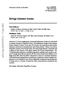
Dirichlet(D-)branes [1] have been necessary ingredients to study non-perturbative dynamics of string theory since their discovery. They are defined as endpoints of open strings. The low-energy effective theory on a D-brane is described by the Dirac-Born-Infeld(DBI) action. String ending on a D-brane can be realized as solitons or solutions with a source term in the DBI action. These solitons are called BIons [2]. Usually these solitons are constructed as deformations of the Dbrane surface such as a spike. It is not easy to construct a string stretched between D-branes as a soliton of the DBI theory. One reason of difficulty is that no DBI action for multiple D-branes is known so far. Solitons resembling with strings ending on D-branes have been found in a field theory framework [3]. They have given an exact solution of vortex-strings ending on a domain wall in a CP 1 nonlinear sigma model. This theory or the CP N extention was known to admit single or multiple domain wall solutions [4, 5, 6]. Assuming the DBI action on the effective action on a single domain wall, they have further shown that that soliton can be identified with a BIon, a soliton on a D2-brane [3], and so have called it a “D-brane soliton”. Later it has been extended to a solution in U(1) gauge theory coupled to two charged Higgs fields [7]. Exact solutions of multiple domain walls have been constructed in U(N) gauge theory in strong coupling limit, by introducing the “moduli matrix” [8]. By extending this method, the most general solutions of D-brane solitons have been constructed [9] which offers exact (analytic) solutions of multiple domain walls with arbitrary number of vortex-strings stretched between (ending on) domain walls, see Fig. 1. Some aspects of these solitons have been studied. We have found an object with a monopole charge which contributes negatively to the total energy of composite solitons in U(1) gauge theory [9]. It has later been called a “boojum” and studied extensively [10]. In the case of U(N) gauge theory a monopole confined by vortices is also admitted [11, 12, 13, 14], which can be understood as a kink in non-Abelian vortices found earlier [15]. The moduli space has been studied [16] for composite solitons consisting of domain walls, vortex-strings and monopoles. See review papers [17, 16, 18, 19] for recent developments of BPS composite solitons. It has been proposed that domain walls actually can be regarded as D-branes after taking into account quantum corrections by loop effect of vortex-endpoints [20] (see also [21]). It has been proposed that this provides some field theoretical model of the open-closed string duality.

1

-10 0 -5 5 10 10 5 0 -5 -10 -20

-10

0

10

20

Fig. 1: An example of exact solution of the D-brane soliton. A same energy surface is plotted. A figure taken from [9].

In this paper we study classical dynamics of D-brane solitons in 3 + 1 dimensions by using two methods and compare their results. One is to use the moduli space (geodesic) approximation found by Manton in studying the monopole dynamics [22, 23]. In this approximation, geodesics on the moduli space of solitons correspond to dynamics or scattering of solitons. So far the moduli approximation has been used to describe classical scattering of particle-like solitons such as monopoles in three space-dimensions, vortices in two space-dimensions [24, 25], and kinks in one space-dimension [26, 6], which are 1/2 Bogomol’nyi-Prasad-Sommerfield (BPS) states. As the first example of composite solitons, it has been recently applied to dynamics of domain wall networks [27, 28], which are 1/4 BPS states [29]. Here we apply it to dynamics of D-brane solitons, vortex-strings stretched between domain walls. The other is to use a charged particle approximation of solitons and a domain wall effective action. It was suggested by Manton that monopoles can be regarded as particles with magnetic and scalar charges [30, 23]. It was used to derive an asymptotic metric on the moduli space of well-separated BPS monopoles [31]. On the other hand, the effective action on a single domain wall is a free Lagrangian of the U(1) Nambu-Goldstone zero mode and the translational zero mode. This U(1) zero mode can be dualized to a U(1) gauge field in the 2+1 dimensional world volume of the wall [3], then the effective Lagrangian becomes a dual U(1) gauge theory plus one neutral scalar field. It has been found by Shifman and Yung [7] that string endpoints can be 2

regarded as electrically charged particles in a dual U(1) gauge theory of the domain wall effective action. We generalize this discussion to N parallel domain walls. As effective theory of well separated N domain walls, we propose U(1)N gauge theory and N scalar fields corresponding to wall positions. Then we use the particle approximation for endpoints of strings on the domain walls. By comparing the moduli metric derived by the moduli approximation for the full 1/4 BPS configurations, we find a good agreement in the asymptotic metric. This is instructive for clarifying similarity or difference between D-branes and field theory solitons. The BPS monopoles can be realized as a D1-D3 bound state, D1-branes stretched between separated D3-branes. The endpoints of the D1-branes at the D3-branes can be regarded as BPS monopoles in the D3-brane effective action [32]. The monopole (or D1-brane) dynamics by the particle approximation in the D3-brane effective theory is parallel to our second derivation of the vortex-string dynamics as the charged particles in the domain wall effective theory. The only difference is the number of codimensions of string-endpoints, which is three for D1-D3 and two for vortex-strings on walls. In fact our asymptotic metric is similar to that of monopoles [30, 31] by replacing 1/r by log r, where r is the distance between solitons. However there exists a crucial difference when N host branes (D3-branes or walls) coincide. The effective theory of D3-branes is in fact U(N) gauge theory with several adjoint Higgs fields, reducing to U(1)N gauge group only when eigenvalues of the adjoint Higgs field (positions of N D3-branes) are different from each other. In contrast to this, our effective theory on domain walls does not become U(N) gauge theory even when domain walls coincide.1 This paper is organized as follows. In Sec. 2.1 we briefly explain the 1/4 BPS equations in the U(NC ) gauge theory with NF hypermultiplets. In Sec. 2.2 we review 1/4 BPS wall-vortex systems in the U(1) gauge theory. In Sec. 3 we first construct a general form of the effective Lagrangian of 1/4 BPS solitons in the U(NC ) gauge theory, by applying the method to obtain a manifestly supersymmetric effective action on BPS solitons [36]. Next we use it to examine normalizability of zero modes of 1/4 BPS wall-vortex systems in the U(1) gauge theory. Here we assume that each vacuum region between two adjacent domain walls has the same number 1

If we consider domain walls with degenerate masses for Higgs scalar fields, we have U (N ) Nambu-Goldstone

modes for coincident domain walls [33, 34, 35]. Taking a duality has been achieved only for 3+1 dimensional wall world-volume, where dual fields are non-Abelian 2-form fields rather than Yang-Mills fields [35].

3

of vortices. It is easy to see that zero modes related to domain walls or vortices with infinite lengths are non-normalizable. We find the center of mass of vortex-strings in each vacuum region is also non-normalizable, and the other zero modes are normalizable. In Sec. 4 we give examples of (1, 1, 1), (2, 2, 2), (0, 2, 0) and (n, 0, n) in the U(1) gauge theory with three flavors admitting two domain walls. Here (n1 , n2 , n3 ) represent configurations in which n1 and n3 strings end on the left (right) domain wall from outside and n2 strings are stretched between the domain walls, see Fig. 2 below. We obtain the effective Lagrangian explicitly in the strong coupling limit as a nonlinear sigma model on the moduli space. In the case of (1, 1, 1), we find the position of the vortex living in the middle vacuum is non-normalizable. We give the physical explanation of the divergence in the effective Lagrangian. In the cases of (2, 2, 2) and (0, 2, 0), the relative positions of vortices in the middle region gives normalizable modes and, we find the 90 degree scattering for head-on collision of those vortices. Metrics of both configurations can be expressed in terms of hypergeometric functions. The (n, 0, n) example is a bit strange in the sense that no vortices can move. Since the region of the middle vacuum is finite in this case, there exists a normalizable moduli parameter for the size of the middle region. We obtain the effective Lagrangian for the modulus. In Sec. 5 we obtain vortex-string dynamics from a dual effective theory on domain walls. A dual effective theory on N well-separated domain walls is U(1)N gauge theory with N real scalar fields parameterizing the wall positions, and endpoints of the vortexstrings can be viewed as particles with scalar charges and electric charges. We obtain a general effective Lagrangian which describes dynamics of charged particles. We find a good agreement to the results obtained by the moduli space approximation of full 1/4 BPS configurations. Sec. 6 is devoted to conclusion and discussion. In Appendix. A, we evaluate the K¨ahler metrics for (2, 2, 2) and (0, 2, 0) configurations. In Appendix. B, the asymptotic K¨ahler metrics are examined. In Appendix. C, we show that the asymptotic metric obtained in Sec. 5 is K¨ahler by writing down the K¨ahler potential explicitly. In Appendix. D, we discuss the dual effective theory on multiple domain walls.

4

2

Composite solitons of walls, vortices, and monopoles

2.1

BPS equations and their solutions

Let us here briefly present our model admitting the 1/4 BPS composite solitons of domain walls, vortices, and monopoles (see [16] for a review). Our model is 3+1 dimensional N = 2 supersymmetric U(NC ) gauge theory with NF (> NC ) massive hypermultiplets in the fundamental representation. The bosonic components in the vector multiplet are gauge fields WM (M = 0, 1, 2, 3), the two real adjoint scalar fields Σα (α = 1, 2), and those in the hypermultiplet are the SU(2)R doublets of the complex scalar fields H i (i = 1, 2), which we express as NC × NF matrices. The bosonic part of the Lagrangian is given by   1 1 MN M α i M i † (2.1) + 2 DM Σα D Σ + DM H (D H ) − V, L = Tr − 2 FM N F 2g g # " 3 1 1 X a 2 V = Tr 2 (Y ) + (H i M − Σ1 H i )(H i M − Σ1 H i )† + Σ2 H i (Σ2 H i )† − 2 [Σ1 , Σ2 ]2 (2.2) g a=1 g
2 where g is a U(N) gauge coupling constant, and we have defined Y a ≡ g2 ca 1NC − (σ a )j i H i(H j )†

with ca an SU(2)R triplet of the Fayet-Iliopoulos (FI) parameters. In the following, we choose

the FI parameters as ca = (0, 0, c > 0) by using SU(2)R rotation without loss of generality. We use the space-time metric ηM N = diag (+1, −1, −1, −1) and the covariant derivatives are defined

as DM Σα = ∂M Σα + i[WM , Σα ], DM H i = (∂M + iWM )H i , and the field strength is defined as

FM N = −i[DM , DN ] = ∂M WN − ∂N WM + i[WM , WN ]. M is a real NF × NF diagonal mass matrix, M = diag (m1 , m2 , · · · , mNF ). In this paper we consider non-degenerate real masses, chosen as m1 > m2 > · · · > mNF . If we turn off all the mass parameters, the moduli space of vacua is the cotangent bundle over the complex Grassmannian T ∗ GrNF ,NC [37]. Once the mass parameters mA (A = 1, · · · , NF ) are turned on and chosen to be fully non-degenerate (mA 6= mB for A 6= B), the almost all points of the vacuum manifold are lifted and only NF !/ [NC !(NF − NC )!] discrete points on the base manifold GrNF ,NC are left to be the supersymmetric vacua [38]. Each vacuum is characterized by a set of NC different indices hA1 · · · ANC i such that 1 ≤ A1 < · · · < ANC ≤ NF . In these discrete vacua, the vacuum expectation values are determined as

2rA 

1rA  √ A H = 0, H = c δ r A, hΣ1 i = diag (mA1 , · · · , mANC ), 5

hΣ2 i = 0,

(2.3)

where the color index r runs from 1 to NC , and the flavor index A runs from 1 to NF . The 1/4 BPS equations for composite solitons of walls, vortices, and monopoles can be obtained by the usual Bogomol’ny completion of the energy density [9, 17, 16, 19] as D2 Σ − F31 = 0, D1 Σ − F23 = 0,
g2 c1NC − HH † = 0, D3 Σ − F12 − 2 D1 H + iD2 H = 0, D3 H + ΣH − HM = 0,

(2.4) (2.5) (2.6)

where H ≡ H 1 , Σ ≡ Σ1 and H 2 , Σ2 have been suppressed since they do not contribute to soliton solutions for c > 0. These equations describe composite solitons consisting of monopoles, vortices with codimensions in the z ≡ x1 + ix2 plane, and walls perpendicular to the x3 direction.2 The Bogomol’ny bound for the energy density E is given as E ≥ tw + tv + tm + ∂m Jm .

(2.7)

Here tw , tv , tm are the energy densities for walls, vortices and monopoles, respectively, given by tw = c ∂3 TrΣ, where Bm =

1 ǫ F 2 mnl nl

tv = −c TrB3 ,

tm =

2 ∂m Tr(ΣBm ), g2

(2.8)

(m, n, l = 1, 2, 3). The monopole charge tm can be either positive or

negative, corresponding to monopoles and boojums, respectively. The last term in Eq. (2.7) containing Jm (m = 1, 2, 3), which are defined by
J1 ≡ Re −iTr(H † D2 H) , J3 ≡ −Tr(H † (Σ − M)H),


J2 ≡ Re iTr(H † D1 H) ,

(2.9)

is a correction term which does not contribute to the total energy. Since Eq.(2.4), which are equivalent to [D1 + iD2 , D3 + Σ] = 0, provides the integrability condition for the operators D1 + iD2 and D3 + Σ, we can introduce an NC × NC invertible complex matrix function S(z, z¯, x3 ) ∈ GL(NC , C) defined by [9]
(D3 + Σ)S −1 = 0 ,
(D1 + iD2 )S −1 = 0 ,

Σ + iW3 ≡ S −1 ∂3 S, ¯ W1 + iW2 ≡ −2iS −1 ∂S, 2

(2.10) (2.11)

When there exists a flux on a domain wall worldvolume, the domain wall is tilted [9] resembling with non-

commutative monopoles.

6

with ∂¯ ≡ ∂/∂ z¯. With the form of Eq.(2.10) and Eq.(2.11), Eq.(2.4) is satisfied, and Eq.(2.6) is solved by H = S −1 (z, z¯, x3 )H0 (z)eM x3 .

(2.12)

Here H0 (z) is an NC × NF matrix whose elements are arbitrary holomorphic functions of z. We call it the “moduli matrix” since it contains all the moduli parameters of solutions as we will see shortly. Let us define an NC × NC Hermitian matrix Ω ≡ SS † ,

(2.13)

invariant under the U(NC ) gauge transformations. The remaining BPS equation (2.5) can be rewritten in terms of Ω as [9]  1  4∂z (Ω−1 ∂¯z Ω) + ∂3 (Ω−1 ∂3 Ω) = 1NC − Ω−1 Ω0 , 2 g c 1 Ω0 ≡ H0 e2M x3 H0† . c

(2.14) (2.15)

This equation is called the master equation for the wall-vortex-monopole system. This reduces to the master equation for the 1/2 BPS domain walls if we omit the z-dependence (∂z = ∂z¯ = 0) while that for the 1/2 BPS vortices if we omit the x3 -dependence (∂3 = 0) and set M = 0. It determines S for a given moduli matrix H0 up to the gauge symmetry S → SU † , U ∈ U(NC ) and then the physical fields can be obtained through Eqs. (2.10), (2.11) and (2.12). The master equation Eq. (2.14) has a symmetry which we call “V -transformations” H0 (z) → V (z)H0 (z),

S(z, z¯, x3 ) → V (z)S(z, z¯, x3 ).

(2.16)

where V (z) ∈ GL(NC , C) has components holomorphic with respect to z. The moduli matrices related by this V -transformation are physically equivalent H0 (z) ∼ V (z)H0 (z) since they do not change the physical fields. Therefore the total moduli space of this system, defined by all topological sectors patched together, is given by a set of the whole holomorphic matrix H0 (z) divided by the equivalence relation H0 (z) ∼ V (z)H0 (z). Therefore the parameters contained in the moduli matrix H0 (z) after fixing the redundancy of the V -transformation can be interpreted as the moduli parameters, namely the coordinates of the moduli space of the BPS configurations.

7

2.2

Composite solitons of vortices and domain walls

The moduli matrix offers a powerful tool to study the moduli space of the 1/4 BPS composite solitons, because it exhausts all possible BPS configurations. In this paper we study the dynamics in the Abelian-Higgs model with NF (≥ 2) flavors, in which the moduli matrix is an NF -vector. To this end we summarize here how the moduli matrix represents 1) the SUSY vacua, 2) 1/2 BPS domain walls, 3) 1/2 BPS vortices and 4) 1/4 BPS composite states. 1) NF discrete SUSY vacua. In the A-th vacuum hAi (A = 1, 2, · · · , NF ), only A-th element is nonzero with the rests being zero, hAi : H0 = (0, · · · , 0, 1, 0, · · · , 0).

(2.17)

2) NF − 1 multiple 1/2 BPS domain walls. When the A-th and the B-th elements (A > B) and the elements between them are nonzero constants in H0 , it represents A−B multiple domain walls interpolating between two vacua hAi and hBi. The most general configurations are obtained when all the elements are nonzero constants: H0 = (h1 , h2 , · · · , hNF ),

hA ∈ C.

(2.18)

If some of {hA } vanish, the corresponding vacua disappear. Namely, the domain walls adjacent to the vacua collapse. In order to estimate the position of the domain wall interpolating between hAi and hA + 1i, let us define the weight of the vacuum hAi by exp(W hAi ) ≡ hA emA x3 .

(2.19)

In the region where the only one of the weights exp(W hAi ) is large, the solution of the master equation Eq. (2.14) is approximately given by Ω ≈ exp(W hAi ). In such regions, the energy density

of the domain wall tw vanishes since it is given by tw = 2c ∂32 log Ω. The A-th domain wall exists

where the weights exp(W hAi ) and exp(W hA+1i ) of the two vacua hAi and hA + 1i are balanced.

Its position x3 = X A can be estimated by A

A

∆mA X + iσ ≃ log



hA+1 hA



,

(2.20)

with ∆mA ≡ mA − mA+1 > 0. Here the imaginary part σ A represents an associated phase modulus of the wall. The tension of this domain wall is c∆mA . 8

3) 1/2 BPS vortices in the vacuum hAi. When only the A-th element hA (z) of H0 is a polynomial function of z with the rests zero, H0 = (0, · · · , 0, hA (z), 0, · · · , 0), hA (z) = vA (z − zhAi1 )(z − zhAi2 ) · · · (z − zhAikA ),

(2.21) (2.22)

it represents multiple vortices in the vacuum hAi extending to infinity (x3 → ±∞). The degree of the polynomials nA = deg[hA (z)] is identical to the number of the vortices in the vacuum hAi, and the zeros zhAi1 , · · · , zhAikA of hA (z) represent the vortex positions. We call the infinitely long straight vortices, generated by the above moduli matrix, the ANO vortices. The tension of each √ vortex is 2πc, and its transverse size is of the order 1/(g c). The ANO vortex becomes singular in the strong gauge coupling limit g → ∞. 4) 1/4 BPS states (D-brane solitons). The most general composite states of vortex-strings ending on (or stretched between) domain walls are given by the moduli matrix H0 = (h1 (z), h2 (z), · · · , hNF (z)),

(2.23)

where the A-th element hA (z) is of the form of Eq. (2.22) with the degree nA . Here nA vortices exist in the vacuum hAi and are suspended between (A − 1)-th and the A-th domain walls for A 6= 1, NF , or ending on the first or the (NF − 1)-th domain wall for A = 1, NF . We denote such D-brane soliton by (n1 , n2 , · · · , nNF ), see Fig. 2. Let us define a z-dependent generalization of the weight of the vacuum hAi by
exp W hAi (z) ≡ hA (z)emA x3 .

(2.24)

Domain walls are curved and their positions in x3 -direction depend on z in general. The zdependent position X A (z, z¯) of the A-th domain wall and its associated (z-dependent) phase σ(z, z¯) can be estimated by equating two weights (2.24), to yield   hA+1 (z) A A . ∆mA X (z, z¯) + iσ (z, z¯) ≃ log hA (z)

(2.25)

One can quickly see an approximate configurations from this rough estimation. Exact solutions and the approximations (2.25) are compared in Fig. 3. If a vortex ends on a domain wall, it pulls the domain wall towards its direction to give the logarithmic bending of the domain wall (2.25).

9

(A + 1)-th wall A-th wall

zhA+2i2

zhA+1i2

zhA+2i1

(A − 1)-th wall zhA−1i2

hA + 2i X A+1 ≃

1 ∆mA+1





log vvA+2 A+1

XA ≃

1 ∆mA

zhAi2

zhA+1i1 zhAi1

hA + 1i

zhA−1i1

log vA+1 vA

hAi

X

A−1

≃

1 ∆mA−1

log v vA A−1

x1 hA − 1i x2

x3

Fig. 2: An example of the D-brane soliton (· · · , nA−1 , nA , nA+1 , nA+2 , · · · ) = (· · · , 2, 2, 2, 2, · · · ) in the U(1) gauge theory.

When the same number of vortices end on the domain wall from both sides, that is, nA = nA+1 , then the domain wall is asymptotically flat A

A

∆mA X (z, z¯) + iσ → log



vA+1 vA



,

as |z| → ∞.

(2.26)

The correction terms of order log z correspond to deformation by the vortices end on the domain walls. We can read the deformation near the i-th vortex at z = zhAii in the vacuum hAi, which ends on the A-th domain wall from the right X vA+1 X A + zhAii − zhA+1ij − log log zhAii − zhAij (2.27) . ∆mA X (zhAii , z¯hAii ) ≃ − log ǫ + log vA j j6=i Here the first term with 0 < ǫ ≪ 1 (UV cut off) comes from the vortex at z = zhAii and the

second term represents the host A-th domain wall. The third and the fourth terms correspond to the deformation by the rest of vortices. The deformation by the rest of vortices ending from the same side make the vortex longer while that by the other vortices ending from the opposite side shorten the vortex, see Fig. 3. 10

x3

x3

x3 6

2 -10

-5

5

10

ÈzÈ

-2

10

4

5

2

-4 -6

-20

-10

10

-8

-5

-10

-10

20

x1

-20

-10

10

20

x1

-2 -4 -6

Fig. 3: The {left, middle, right} panel shows {(0,1), (1,1), (0,2)} configuration, respectively. The solid line is the exact solution for the equal energy density contour of E = 1/2 while the broken line is an approximate curve given by Eq. (2.25). Gray long-dashed lines correspond to the configurations that one of two vortices is removed away to infinity. The parameters are chosen to be c = 1 and M = diag(1/2, −1/2). Furthermore, one can estimate transverse size of vortices as follows. If we look at region sufficiently away from domain walls, we can ignore x3 dependence of the configurations. In such a region one can take a slice with fixed x3 and can regard the configuration as semilocal vortices in 2+1 dimensions. The configuration is determined by Ω0 typically taking the form of Ω0 = |z − z0 (x3 )|2 + |a(x3 )|2 ,

(2.28)

up to an overall factor independent of z. Here z0 stands for the position and |a| for the transverse size of the semilocal vortex. Let us show two concrete examples of the D-brane soliton (n1 , · · · , nNF ). • (n1 , n2 ) = (0, 1) case: For instance, we consider the mass matrix M = diag.(m/2, −m/2) with the moduli matrix H0 = (1, z − z0 ) and obtain


Ω0 = emx3 + |z − z0 |2 e−mx3 = e−mx3 |z − z0 |2 + e2mx3 .

(2.29)

The (z-dependent) transverse size can be read as |a(x3 )| = emx3 , see Fig. 3 (left-most). • (n1 , n2 , n3 ) = (1, 1, 1) case: For instance, we consider the mass matrix M = diag.(m/2, 0, −m/2) with the moduli matrix H0 = (z − z1 , eml/4 (z + z1 ), z − z1 ) for the coincident outer vortices Ω0 = |z − z1 |2 emx3 + eml/2 |z + z1 |2 + |z − z1 |2 e−mx3 = 2|z − z1 |2 cosh mx3 + eml/2 |z + z1 |2 # " 2  2 ! A − B A − B |z1 |2 , z1 + 1 − = (A + B) z − A+B A+B 11

(2.30)

with A ≡ 2 cosh mx3 and B ≡ eml/2 . The physical meaning of l is the distance between two

domain walls. The (z-dependent) position of the vortex is given by z0 (x3 ) = A−B z and their A+B 1 q
2 . Therefore, one can see that z0 (x3 → ±∞) → z1 sizes are by |a(x3 )| = |z1 | 1 − A−B A+B

and the position of the middle vortex is z0 (x3 = 0) = −z1 if l ≫ 1. The size of the outer q m l vortices reduces 2|z1 | B ∼ 2|z1 |e 2 ( 2 −|x3 |) → 0 as |x3 | → ∞. On the other hand, if the A

separation of the two walls are sufficiently large so that B ≫ A, the size is estimated by q m l A 2|z1 | B ∼ 2|z1 |e− 2 ( 2 −|x3|) . Thus the center of the middle vortex (x3 = 0) has the smallest size |a(x3 = 0)| = 2|z1 |e−ml/2 . It is exponentially small with respect to the wall distance l,

but still finite. However, the size becomes zero when all the vortices are coincident (z1 = 0). The vortices ending on the domain walls are not the usual ANO vortices. They are also deformed by domain walls and their transverse sizes are not constant along x3 any more. The sizes depend on the positions the vortices. The ANO vortices appear at z = z1 , z2 , · · · , zk′ only when all elements of the moduli matrix have common zeros as H0 (z) = (z − z1 )(z − z2 ) · · · (z − zk′ ) × H0′ (z),

(2.31)

without poles in H0′ (z). We call such moduli matrix as factorizable. In the strong gauge coupling limit, these ANO vortices become singular. On the other hand, the other general vortices ending on (stretched between) domain walls remain regular with finite transverse sizes in the strong coupling limit.

3

Effective Lagrangian of 1/4 BPS wall-vortex systems

3.1

General form of the effective Lagrangian

Now let us construct the effective Lagrangian of the full 1/4 BPS composite solitons.3 Zero modes on the background BPS solutions will play a main role in the effective theory while all the massive modes will be ignored in the following. As we will see shortly, the composite solitons have normalizable zero modes, and also non-normalizable zero modes. Only the normalizable 3

Our main interest in this paper is dynamics of vortices between domain walls in the Abelian gauge theory.

However, the general formula obtained in this section can be applied to other composite solitons in non-Abelian gauge theory.

12

zero modes can be promoted to dynamical degrees of freedom in the effective theory. In this subsection we construct a formal form of the effective Lagrangian without identifying which zero modes are normalizable. We will discuss the problem of the normalizability in the next subsection by extending our method to obtain a manifestly supersymmetric effective action on BPS solitons [36]. If there are normalizable zero modes φi, we can give them weak dependence on time (slow move approximation `a la Manton [22, 23])

H0 φi → H0 φi (t) .

(3.1)

We introduce “the slow-movement order parameter” λ, which is assumed to be much smaller than the other typical mass scales in the problem. There are two characteristic mass scales: one √ is mass difference |∆m| of hypermultiplets, and the other is g c in front of the master equation. Therefore, we assume that √ λ ≪ min( |∆m| , g c ).

(3.2)

The non-vanishing fields in the 1/4 BPS background have contributions independent of λ, namely we assume that H 1 = O(1),

Wm = O(1),

Σ1 = O(1).

(3.3)

The derivatives of these fields with respect to time are assumed to be of order λ expressing the weak dependence on time. The vanishing fields in the background can now have non-vanishing values, induced by the fluctuations of the moduli parameters of order λ. Therefore, we assume that ∂0 = O(λ),

H 2 = O(λ),

W0 = O(λ),

Σ2 = O(λ).

(3.4)

Then the covariant derivative D0 = O(λ) has consistent λ dependence. If we expand the full equations of motion of the Lagrangian (2.1) in powers of λ, we find that the O(1) equations are automatically satisfied due to the BPS equations (2.4)-(2.6). The next leading O(λ) equation is the equation for W0 , which is called the Gauss law 0=−

2 2i D F + [Σ1 , D0 Σ1 ] + i(H 1 D0 H 1† − D0 H 1 H 1† ), m m0 2 2 g g 13

(3.5)

with m = 1, 2, 3. In order to obtain the effective Lagrangian of order λ2 of the composite solitons, we have to solve this equation and determine the configuration of W0 . As a consequence of Eq.(3.1), the moduli matrix H0 (φi ) depends on time through the timedependent moduli parameter φi (t). Note that for the fields which depend on time only through φi (t), the derivatives with respect to time satisfy ∂0 = δ0 + δ0† ,

(3.6)

where we have defined the differential operators δ0 and δ0† by δ0 ≡

X i

∂0 φi

∂ , ∂φi

δ0† ≡

X i

∂ ∂0 φ¯i ¯i , ∂φ

(3.7)

in order to distinguish chiral φi and anti-chiral φ¯i multiplets of preserved supersymmetry. Using these operators, the Gauss law (3.5) can be solved to yield [36] W0 = i(δ0 S † S †−1 − S −1 δ0† S).

(3.8)

The effective Lagrangian is obtained by substituting these solutions into the fundamental Lagrangian (2.1) and integrating over the codimensional coordinates x1 , x2 and x3 . We retain the terms up to O(λ2 ) since we are interested in the leading nontrivial part in powers of λ, and we ignore total derivative terms which do not contribute to the effective Lagrangian. Then the effective Lagrangian for the composite solitons can be obtained as dφi dφ¯j Leff = Ki¯j dt dt"   Z 1 3 −1 2 Ki¯j = d x Tr ∂i ∂¯j c log Ω + 2 (Ω ∂3 Ω) 2g #  4 + 2 ∂z¯(Ω∂i Ω−1 )∂¯j (Ω∂z Ω−1 ) − ∂z¯(Ω∂z Ω−1 )∂¯j (Ω∂i Ω−1 ) . g

(3.9)

(3.10)

This is a nonlinear sigma model whose target space is the moduli space of the 1/4 BPS configurations. The metric on the moduli space is a K¨ahler metric, which can be obtained from the following K¨ahler potential4   Z Z t Z 4 1 1 −ψ ψ 2 −sLψ 3 −ψ ¯ dt ds ∂ψe ∂ψ (3.11) K = d x Tr c ψ + c e Ω0 + 2 (e ∂3 e ) + 2 2g g 0 0 4

Although this K¨ ahler potential is divergent, it can be made finite without changing the K¨ahler metric by the

K¨ahler transformation, namely by adding terms f (x, φ) and f (x, φ) which are (anti-)holomorphic with respect to the normalizable moduli parameters to the integrand of Eq. (3.11).

14

where ψ ≡ log Ω and the operation Lψ is defined by Lψ × X = [ψ, X].

(3.12)

This general form reduces to the effective Lagrangian for either 1/2 BPS domain walls or 1/2 BPS vortices if one considers the moduli matrix of the corresponding 1/2 BPS states.

3.2

Normalizability of zero modes

The moduli matrix contains both normalizable and non-normalizable zero modes because it exhausts all possible configurations. There exist two kinds of zero modes appearing in the moduli matrix as we saw in the previous section. One is related to positions and phases of domain walls which form complex numbers. The other represents the positions of vortices. In general zero modes changing the boundary conditions at infinities are non-normalizable. For examples, zero modes related to domain walls or vortices with infinite lengths are apparently non-normalizable because the infinite extent of the solitons brings divergence in the integration. However the opposite is not true; zero modes fixing the boundary conditions are not always normalizable but sometimes are non-normalizable. Purpose of this section is to examine if zero modes for vortices with finite lengths stretched between domain walls are normalizable or not. Now let us analyze the divergences of the K¨ahler potential (3.11) in order to find out which modes are normalizable and which are not. Since the solutions of the master equation (2.14) have been assumed to be smooth, the divergences of the K¨ahler potential can appear only from the integration around the boundaries at infinity. The composite solitons have two kinds of boundaries: one is along |z| → ∞ where we see no vortices, and the other is along x3 → ±∞ where we see no domain walls. We will discuss the behaviors of solutions near these two boundaries separately. From now on, we consider Abelian gauge theories (NC = 1) for simplicity. First let us consider the boundary along |z| → ∞. The master equation (2.14) can be rewritten in terms of ψ = log Ω as

4∂z ∂z¯ + ∂32 ψ = g 2 c 1 − e−ψ Ω0

(3.13)

For simplicity, we will assume all domain walls are asymptotically flat, that is, each vacuum has 15

the same number of vortices. Let us denote the number of vortices as k. Then Ω0 is given by N

Ω0

F X 1 2M x3 † H0 e H0 = |hA (z)|2 e2mA x3 ≡ c A=1

(3.14)


hA (z) = vA (z − zhAi1 )(z − zhAi2 ) · · · (z − zhAik ) = vA z k − aA z k−1 + · · · .

(3.15)

The moduli parameter vA controls the weight of the vacuum hAi in Eq. (2.24), and thus is related to positions of the domain walls separating the vacuum hAi from the adjacent vacua. The moduli parameters aA are related to the center of mass ZAc of vortices in the vacuum hAi as ZAc ≡

zhAi1 + · · · + zhAik aA = . k k

(3.16)

Let us introduce new functions defined as ˜ A (z) ≡ hA (z) , h zk ˜ 0 (z, z¯, x3 ) ≡ Ω0 (z, z¯, x3 ) , Ω |z|2k ˜ z¯, x3 ) ≡ ψ(z, z¯, x3 ) − log |z|2k . ψ(z,

(3.17) (3.18) (3.19)

The master equation (3.13) does not change in terms of these functions except for the appearance of the delta function5 in z. Since we are interested in the boundary along |z| → ∞, let us ignore the delta function in the following discussion.  
˜˜ 4∂z ∂z¯ + ∂32 ψ˜ = g 2 c 1 − e−ψ Ω 0 .

(3.20)

˜ 0 becomes If we take the limit |z| → ∞, Ω

˜ 0 → Ω0w ≡ Ω

NF X A=1

|vA |2 e2mA x3 ,

(3.21)

which is nothing but the source for domain walls without vortices. Therefore, the solution ˜ z¯, x3 ) approaches the domain wall solution in large |z| region. We denote it as ψw (x3 ) ψ(z, ˜ z¯, x3 ) → ψw (x3 ) ψ(z,

as |z| → ∞.

(3.22)

˜ 0 can be Now let us analyze the effects of vortices on the asymptotic behavior. Note that Ω expanded as ˜ 0 (z, z¯, x3 ) = Ω0w (x3 ) − Ω 5

NF X A=1

|vA |

2

a ¯A  2mA x3 e +O + z z¯

a

A



1 z2



.

(3.23)

This redefinition transform our master equation to the so-called Taubes’s equation [39] in the case of vortices

without domain walls.

16

We will assume ψ˜ can be also expanded as ¯ 3) ˜ z¯, x3 ) = ψw (x3 ) + ϕ(x3 ) + ϕ(x +O ψ(z, z z¯



1 z2



.

(3.24)

If we substitute the asymptotic forms (3.23) and (3.24) into the master equation (3.20), and expand it in terms of z, we find that O(1) equation gives the master equation for domain walls

and O(z −1 ) equation gives


∂32 ψw = g 2 c 1 − e−ψw Ω0w ,

∂32 ϕ = g 2c Ω0w ϕ +

NF X A

|vA |2 aA e2mA x3

(3.25)

!

e−ψw .

(3.26)

Using the equation (3.25), we can find the solution of the equation (3.26) as ϕ(x3 ) = −

NF X

vA aA

A=1

∂ψw (x3 ) . ∂vA

(3.27)

Let us now substitute these asymptotic behaviors (3.24) and (3.27) into the K¨ahler potential (3.11). Using the fact that the solution of the master equation is the extremum of the K¨ahler potential, we obtain K =

Z

d2 z

 ! NF 1 X 1 ∂ 2 Kw Kw + 2 +O (aA vA )(¯ aB v¯B ) |z| A,B=1 ∂vA ∂¯ vB z4

2

≃ πL Kw + 2π log L

NF X

(aA vA )(¯ aB v¯B )

A,B=1

∂ 2 Kw + const. + O(L−2 ) ∂vA ∂¯ vB

where L is the infrared cutoff |z| < L, and Kw is the K¨ahler potential for domain walls   Z 1 −ψ ψ 2 Kw (vA , v¯A ) = dx3 Tr c ψw + c e−ψw Ω0w + 2 (e w ∂3 e w ) 2g   NX −1 2 F vA+1 c , log ≈ ∆mA vA

(3.28)

(3.29)

A=1

where the last line is valid for well-separated walls. From the K¨ahler potential Eq. (3.28) we find that the leading terms in the K¨ahler metric for the moduli parameters vA are proportional to L2 and diverge in the limit L → ∞. Therefore moduli parameters vA , which are contained in Ω0w , correspond to non-normalizable zero modes. This is because the infinitely extended domain walls move with infinite kinetic energy when the parameters vA vary. However, the above result 17

says that the center of mass positions of vortices, aA , in each vacuum are also non-normalizable even if the vortices have finite lengths. The divergent part of the effective Lagrangian associated with the motion of the parameters aA is NF NX F −1 X daA d¯ 1 aB ∂ 2 Kw 2π log L vA v¯B ≈ πc log L dt dt ∂vA ∂¯ vB ∆mA A,B=1 A=1

daA daA+1 2 dt − dt .

(3.30)

The intuitive explanation is given as follows. In the presence of vortices, the positions of domain walls actually depend on the positions of vortices. For example, the position and the corresponding phase of the A-th domain wall interpolating the two vacua hAi and hA + 1i is given by A

A

∆mA X (z, z¯) + iσ (z, z¯) = log



vA+1 vA



+ log



 z k − aA+1 z k−1 + · · · . z k − aA z k−1 + · · ·

(3.31)

Let us perturb the center of mass positions of vortices aA and aA+1 with vA and vA+1 fixed, to yield δ(∆mA X A + iσ A ) = δaA

z k−1 z k−1 − δa . A+1 k z k − aA z k−1 + · · · z − aA+1 z k−1 + · · ·

(3.32)

Therefore, if aA is promoted to a dynamical degrees of freedom to have the weak dependence on time, there appears kinetic energy of domain wall with the tension TA ≡ c∆mA  2 Z daA daA+1 2 πc dX A 2 TA . dz ≈ log L − 2 dt 2∆mA dt dt

(3.33)

The same amount of kinetic energy appears from the phase σ A of the domain wall. Thus the

non-normalizability of aA given in Eq. (3.30) can be understood as the divergent kinetic energy of domain walls. Now let us consider the boundaries along x3 → ±∞ directions. As in the previous case, we define the following new functions for the limit x3 → +∞ ˇ 0 (z, z¯, x3 ) ≡ Ω0 (z, z¯, x3 )e−2m1 x3 = Ω ˇ z¯, x3 ) ≡ ψ(z, z¯, x3 ) − 2m1 x3 . ψ(z,

NF X

A=1

|hA (z)|2 e−2(m1 −mA )x3 ,

(3.34) (3.35)

Note that we have chosen the mass parameters such that m1 > m2 > · · · > mNF . The master equation (3.13) does not change in terms of these functions as before. If we take the limit ˇ 0 becomes x3 → ∞, Ω ˇ 0 → Ωv ≡ |h1 (z)|2 , Ω 0 18

(3.36)

ˇ z¯, x3 ) which is nothing but the source for vortices in vacuum h1i. Therefore, the solution ψ(z, approaches the vortex solution in large x3 region, which we denote as ψv (z, z¯) ˇ z¯, x3 ) → ψv (z, z¯) ψ(z,

as x3 → ∞,
4∂z ∂z¯ψv = g 2 c 1 − e−ψv Ωv0 .

(3.37) (3.38)

ˇ 0 behaves We are interested in the effects of domain walls on the asymptotic behavior. Note that Ω ˇ 0 = |h1 (z)|2 + |h2 (z)|2 e−2(m1 −m2 )x3 + · · · Ω

(3.39)

in large x3 region. The second term is strongly suppressed by the exponential factor in contrast ˇ z¯, x3 ) should also behave as to the previous case. The solution ψ(z, ˇ z¯, x3 ) = ψv (z, z¯) + φ(z, z¯)e−mv x3 + O(e−2mv x3 ) ψ(z,

(3.40)

where mv stands for the lowest mass scale of the bulk modes in the right most vacuum h1i. Since the second term is exponentially suppressed and does not give a divergence, the parameters contained in the function φ(z, z¯) correspond to normalizable zero modes. Therefore, only the function ψv (z, z¯) has non-normalizable zero modes, which are positions of vortices living in vacuum h1i. The same argument holds for x3 → −∞ direction. In summary, in the case of flat domain walls, non-normalizable zero modes are positions of domain walls vA , the center of mass of vortices in each vacuum ZAc = aA /nA , and positions of infinitely long vortices zh1ii and zhNF ii in vacuum h1i and vacuum hNF i, respectively.

4

Dynamics of 1/4 BPS wall-vortex systems

Now let us construct the effective Lagrangian of vortices between domain walls. We will discuss the Abelian gauge theory with three flavors. The mass parameters are taken as M = diag ( m2 , 0, − m2 ), and we denote the numbers of vortices in three vacua by (n1 , n2 , n3 ). In what follows, we will take the strong gauge coupling limit (g → ∞) in order to calculate the effective action analytically. In the strong coupling limit, the master equation Eq. (2.14) becomes an algebraic equation and analytically solved as Ω = Ω0 ≡

1 H0 e2M x3 H0† . c 19

(4.1)

The K¨ahler metric Eq. (3.10) also takes a simple form in the strong coupling limit Z Ki¯j = c d3 x ∂i ∂¯j log det Ω0 .

(4.2)

Although the ANO vortices linearly extending to infinity like Eq.(2.31) shrink to singular con√ figurations since their sizes 1/(g c) tend to zero in this limit, vortex strings with finite length between domain walls do not (its size behaves as e−mL where L is separation between walls). Therefore we can construct low energy effective theories for vortex strings between domain walls in the strong coupling limit.

4.1

Numbers of vortices: (1,1,1)

First let us consider the case in which each vacuum has a single vortex. This configuration admits no normalizable zero modes. However, it will give us an explicit example of the non-normalizable modes which we have discussed in Sec.3.2. The general form of the moduli matrix is given by H0 =

√


c v1 (z − zh1i1 ), v2 (z − zh2i1 ), v3 (z − zh3i1 ) .

(4.3)

Since we are interested in the vortex in vacuum h2i, we set zh1i1 = zh3i1 = 0 and v1 = v3 = 1, and define v2 ≡ v and zh2i1 ≡ z0 H0 =

√

c (z, v(z − z0 ), z) .

(4.4)

The positions of domain walls can be estimated by weights of vacua (2.24). Both domain walls are asymptotically flat, and the asymptotic distance between these domain walls, that is, the length of the vortex in vacuum h2i, is given by lh2i =

4 log |v|. m

(4.5)

Energy densities of configurations in a plane containing vortices are shown for several values of moduli parameters in Fig.4. Now we give the weak time dependence to z0 , and investigate the dynamics of the middle vortex. The explicit solution of the master equation (2.14) can be obtained in the strong coupling limit g → ∞ as Ω → Ω0 = |z|2 emx3 + |v|2 |z − z0 |2 + |z|2 e−mx3 . 20

(4.6)

v = e8 , z0 = 20

v = e8 , z0 = 5

v = e5 , z0 = 5

v = e5 , z0 = 20

Fig. 4: The energy densities in a plane containing vortices in the strong coupling limit g → ∞ with c = 1 and m = 1. Vertical lines are walls and horizontal lines are vortices.

Let us substitute this solution into the K¨ahler metric (4.2). Leaving the integration along the x3 -coordinate, the K¨ahler metric can be calculated as Z 2|vz|2 cosh(mx3 ) 3 Kz0 z¯0 ≡ c d x (|v|2 |z − z0 |2 + 2|z|2 cosh mx3 )2 " Z L2 |v|2 (|v|2 − 2 cosh mx3 ) 2|v|2 cosh mx3 = πc dx3 log + (2 cosh mx3 + |v|2)2 |z0 |2 (2 cosh mx3 + |v|2 )2  # 2|v|2 cosh mx3 2|v|2 cosh mx3 log , − (2 cosh mx3 + |v|2)2 (2 cosh mx3 + |v|2 )2

(4.7)

where L is the infrared cutoff in the z-plane |z| < L. As we saw in the previous section, the K¨ahler metric contains the logarithmic divergence. The complicated metric (4.7) reduces to a simple form when we take the limit of |v| → ∞   4 4 4 Kz0 z¯0 ≈ πc log |v| − log |z0 | + log L + const. . m m m

(4.8)

The physical meaning of the metric is clear in this form. Since the tension of the vortex is 2πc and its length is given in Eq. (4.5), the first term in equation (4.8) corresponds to kinetic energy of the vortex. According to equation (3.33) and the following comments, the kinetic energy of two domain walls can be calculated as Twall =

dz0 d¯ z0 4πc log L , m dt dt

(4.9)

where we have identified z0 = a2 and ∆mA = m/2 in Eq. (3.33). This coincides with the third term in equation (4.8). This is the origin of the non-normalizability of z0 . Note that the moduli space has the singularity at z0 = 0. This is because we have fixed the vortices in vacuum h1i and vacuum h3i at the same position. When the vortex in h2i also comes 21

to the same position, they result in a single ANO vortex which is infinitely long and becomes √ singular in the strong coupling limit with its shrinking size 1/(g c) → 0. The singularity can be removed by dislocating the outer vortices. We will discuss this issue in the next example.

4.2

Numbers of vortices: (2,2,2)

Let us next consider the case in which each vacuum has a pair of vortices. The general form of the moduli matrix is given by  √  H0 = c v1 (z − zh1i1 )(z − zh1i2 ), v2 (z − zh2i1 )(z − zh2i2 ), v3 (z − zh3i1 )(z − zh3i2 ) .

(4.10)

Since we are interested in the relative motion of vortices in vacuum h2i, we set zh1ii = 0 = zh3ij and v1 = v3 = 1, and define v2 ≡ v and zh2i1 = −zh2i2 ≡ z0 H0 =

√


c z 2 , v(z 2 − z02 ), z 2 .

(4.11)

The distance between two domain walls is also given by equation (4.5) in the present case. Energy densities of configurations in a plane containing vortices are shown for several values of moduli parameters in Fig.5.

v = e8 , z0 = 20

v = e8 , z0 = 5

v = e5 , z0 = 5

v = e5 z0 = 20

Fig. 5: The energy densities in a plane containing vortices in the strong coupling limit g → ∞ with c = 1 and m = 1. Vertical lines are walls and horizontal lines are vortices.

Now let us give the weak time dependence to z0 , and investigate the dynamics of the middle vortices. The explicit solution of the master equation (2.14) can be obtained in the strong coupling limit g → ∞ Ω → Ω0 = |z|4 emx3 + |v|2 |z 2 − z02 |2 + |z|4 e−mx3 . 22

(4.12)

Let us substitute this solution into the K¨ahler metric (4.2). After integrating the z-coordinates, we obtain the K¨ahler metric Kz0 z¯0 = 2πc

Z

dx3 kE(k)

(4.13)

where E(k) is the complete elliptic integral of the second kind E(k) ≡

Z

π 2

dθ 0

p 1 − k 2 sin2 θ,

(4.14)

with the x3 dependent parameter k k=



|v|2 2 cosh mx3 + |v|2

1/2

.

(4.15)

The metric does not depend on z0 and its value can be written as a sum of the hypergeometric functions (see Appendix A). The asymptotic value of this metric for large |v| is given by (see Appendix B) Kz0 z¯0 ≈

8πc log |4v|. m

(4.16)

The leading term in the effective Lagrangian coincides with the kinetic energy of two vortices with length lh2i = Leff

2 m

log |v|2 and tension Tv = 2πc     8πc 16πc 16πc 2 ≈ log |v| + log 2 |z˙0 | = Tv lh2i + log 2 |z˙0 |2 , m m m

(4.17)

The independence of Leff on the IR cutoff L shows the normalizability of the moduli z0 . Therefore it makes sense to consider its dynamics. Since we cannot distinguish two vortices, the geometry of the moduli space is a cone, C/Z2 . Here Z2 denotes the exchange of the vortices and acts on the coordinate as z0 → −z0 . In fact, a good coordinate of the moduli space is not z0 but z02 , which appears naturally in the moduli matrix (4.11). The moduli space has the singularity at z0 = 0. As we explained in the previous section, this is because we have fixed the outer vortices at the same position. When the vortices in vacuum h2i also come to the same position, they result in two ANO vortices which are singular in the strong coupling limit g → ∞. The singularity can be removed by dislocating the outer vortices. For instance, let us consider the moduli matrix given in the form H0 =

√


c (z − z1 )2 , v(z 2 − z02 ), (z + z1 )2 . 23

(4.18)

The vortices in vacuum h1i are located at z = z1 , and the vortices in vacuum h3i are at z = −z1 . The K¨ahler metric in strong coupling limit is given as Z 4|v|2|z0 |2 (|z − z1 |4 emx3 + |z + z1 |4 e−mx3 ) . Kz0 z¯0 = c d3 x (|z − z1 |4 emx3 + |v|2|z 2 − z02 |2 + |z + z1 |4 e−mx3 )2 The metric starts at O (|z0 |2 ), and can be expanded around z0 = 0 as   ¯ z¯2 + O(|z0 |4 ) dz0 d¯ z0 ds2 ≃ |z0 |2 A + Bz02 + B 0   ¯ + O(|Z|2 ) dZdZ, ¯ = A + BZ + BZ

(4.19)

(4.20)

where Z ≡ z02 is a good complex coordinate on the moduli space. Since the constant A ≡ (Kz0 z¯0 /2|z0 |2 )|z0 =0 is non-zero, the scalar curvature does not diverge at Z = 0. Therefore, the

moduli space is non-singular at the origin, and the vortices scatter with right-angle in head-on collisions. On the other hand, the asymptotic metric for |v|2 ≫ 1 ≫ |z1 /z0 | is given by (see Appendix B) Kz0 z¯0

4vz02 8πc . log 2 ≈ m z0 − z12

(4.21)

This coincides with Eq. (4.17) when z1 = 0. The leading term is again identified with the kinetic term of the vortex of length lh2i =

4.3

2 m

log |v|2 .

Numbers of vortices: (0,2,0)

Let us next consider the case in which only the middle vacuum has a pair of vortices. This is the case where walls are not asymptotically flat, but may be useful as a building block for more complicated configurations. The general form of the moduli matrix is given by H0 =

√


c v1 , v2 (z − zh2i1 )(z − zh2i2 ), v3 .

(4.22)

We are interested in the relative motion of vortices in vacuum h2i. Although we have not discussed the cases in which domain walls are logarithmically bending in Sec. 3.2, it turns out that the relative motion of the two vortices is normalizable zero mode even in such cases. Let us set v1 = v3 = 1, zh2i1 = −zh2i2 ≡ z0 and v2 ≡ v H0 =

√

c ( 1, v(z − z0 )(z + z0 ), 1 ) .

(4.23)

Energy densities of configurations in a plane containing vortices are shown for several values of moduli parameters in Fig.6. 24

v = e4 , z0 = 20

v = e4 , z0 = 5

v = e4 , z0 = 0

v = e2 , z0 = 0

Fig. 6: The energy densities in a plane containing vortices in the strong coupling limit g → ∞ with c = 1 and m = 1. Vertical lines are walls and horizontal lines are vortices. Now let us give the weak time dependence to z0 , and investigate the dynamics of the middle vortices. The explicit solution of the master equation (2.14) can be obtained in the strong coupling limit g → ∞ Ω → Ω0 = emx3 + |v|2 |z 2 − z02 |2 + e−mx3 .

(4.24)

Let us substitute this solution into the K¨ahler metric (4.2). After integrating the z-coordinates similarly to the case of the number of vortices (2, 2, 2) in the previous subsection, we obtain the K¨ahler metric as an integral over the complete elliptic integral of the second kind E(k) defined in Eq. (4.14) Kz0 z¯0 = 2πc

Z

dx3 kE(k),

with k =



|vz02 |2 2 cosh mx3 + |vz02 |2

1/2

.

(4.25)

The metric has the same form as that of the previous example (4.13). However, the variable k in E(k) is now defined differently from the case of (2, 2, 2), v is now replaced by vz02 . Integrating over x3 , we obtain the K¨ahler metric as a sum of the hypergeometric functions (see Appendix A). If we expand the K¨ahler metric around |vz02 |2 = 0, we obtain   3 π2c 3 2 2 2 2 2 2 4 dx = 2Kz0 z¯0 dz0 d¯ z0 → Γ(1/4) − Γ(3/4) |vz0 | + O(|vz0 | ) vz02 dz0 d¯ z0 m 2   3 π 2 |v|c 3 2 2 2 4 ¯ = Γ(1/4) − Γ(3/4) |vZ| + O(|vZ| ) dZdZ. (4.26) 4m 2

Since the coordinate Z ≡ z02 is a good coordinate even at the origin, it shows that the moduli space is non-singular at the origin and the vortices scatter with right-angle in head-on collisions. If we take the opposite limit |vz02 |2 → ∞, the metric can be calculated as (see Appendix B) Kz0 z¯0 ≈

8πc log |4vz02 |. m 25

(4.27)

Since the domain walls are logarithmically bending in the present case, the definition of the distance between domain walls is not clear. However, at the center of mass of two vortices, the distance between domain walls is given by lh2i =

4 log |vz02 |. m

(4.28)

It can be considered as the typical lengths of the vortices (see Fig.6). Therefore, the above asymptotic metric (4.27) can be understood as the kinetic energy of two vortices. Fig. 7 shows a numerically calculated metric and the moduli space embedded into R3 .

80

K

60

z0 z0 40

20

0.00

0.01

0.02

0.03

0.04

0.05

0.06

z0j

j

(a)

(b)

Fig. 7: A metric of the moduli space for c = 1, m = 1, v = e8 . (a) Numerically calculated metric (solid line) and the asymptotic metric Kz0 z¯0 ≈

8πc m

log |4vz02 | (|vz02 | → ∞) (dashed line). (b) The

moduli space isometrically embedded into three dimensional Euclidean space R3 .

4.4

Numbers of vortices: (n, 0, n)

In Sec. 3.2 we have seen that the moduli parameters vA (A = 1, · · · , NF ) correspond to nonnormalizable zero modes if there exist the same number of vortices in each vacuum region. In fact, this is not necessarily the case if there exist different numbers of vortices in each vacuum region. The simplest such example is the configuration described by the following moduli matrix H0 = (z n , v, z n ).

(4.29)

The K¨ahler metric for the moduli parameter v is finite for n ≥ 2. The relative distance of two walls are determined from Eq. (2.25) as ∆X(z, z¯) = 26

4 m

log |v/z n |. Therefore, in the region

(a) v = 50

(b) v = 200

(c) v = 800

(d) v = 3200

Fig. 8: The energy densities in a plane containing vortices in the strong coupling limit g → ∞ with m = 1, c = 1, n = 2. Vertical lines are walls and horizontal lines are vortices.

1

|z| > |v| n , two walls are compressed into one wall located at x3 = 0 and its position is unchanged under the variation of the moduli parameter v → v + δv. Several plots of the energy densities are shown in Fig. 8. The K¨ahler metric for the moduli parameter v is given in the strong coupling limit by Kv¯v = c

Z

2

1 2 ) 2|z|2n cosh(mx3 ) π 2 c |v| n −2 Γ( 2n dx = 1 . 2n 2 2 2 (2|z| cosh(mx3 ) + |v| ) 2n m sin(π/n) Γ( n ) 3

(4.30)

1

In terms of the coordinate u ≡ v n , the metric can be written as ds2 = 2Kv¯v dvd¯ v =

1 2 Γ( 2n ) π2c u. 1 dud¯ m sin(π/n) Γ( n )

(4.31)

The moduli space is a cone C/Zn and has a singularity at v = 0. In the limit v → 0, the moduli matrix can be factorized as H0 = (z 2n , v, z 2n ) → z 2n (1, 0, 1).

(4.32)

This indicates the appearance of ANO vortices in the limit v → 0. The existence of the singularity in the moduli space reflects the fact that the vortices become ANO vortices which are singular in the strong coupling limit g → ∞.

5

Vortex dynamics in a dual effective theory on walls

So far, we have calculated the metric on the 1/4 BPS moduli space and investigated the dynamics of vortices suspended between the domain walls, using the moduli space approximation. Now let us obtain the vortex dynamics from another point of view. 27

5.1

General formalism

Let us first consider the single vortex ending on the single domain wall in the minimal AbelianHiggs model with NF = 2 and see how the vortex ending on the wall appear in the effective theory on the domain wall worldvolume. The 1/2 BPS domain wall is described by a single complex parameter φ = e∆mX+iσ ∈ C∗ ≃ C − {0} ≃ R × S 1 in the moduli matrix H0 = (h1 , h2 ) ≃ (1, φ), see Eq. (2.18). The real part X corresponds to the position of the domain wall, see Eq. (2.20), and σ is its phase. The effective theory on the wall turned out to be a free theory   1 c∆m 2 2 (∂µ X) + (∂µ σ) Lw = 2 ∆m2

(5.1)

via the generic expression Eq. (3.11) [36, 35] Kw =


2 c log |φ|2 4∆m

(5.2)

The moduli matrix given in Eq. (2.23) tells us that we should identify the vortex ending on the wall at z = z0 as the following configuration φ(z, z¯) = e∆mX(z,¯z )+iσ(z,¯z ) = e∆mX0 +iσ0

(z − z0 ) , L

(5.3)

where we have introduced a “boundary” at |z| = L ≫ |z0 | in the z-plane for later convenience. The parameter L plays the role of the cutoff for the IR divergence of the non-normalizable modes. The constants X0 and σ0 respectively represent the position and the phase of the background domain wall at z = L + z0 . Notice that under the identification we have added two points φ = 0, ∞ (X = ±∞) to C∗ resulting in the target space CP 1. In this sense, the above realization

of the vortex is thought of as the 1/2 BPS lump on the domain wall effective action.6 Let us

set X0 =

1 ∆m

log L, σ0 = 0 and z0 = 0 in the following for simplicity. The vortex causes the

logarithmic bending of the domain wall X=

1 1 log |φ| = log |z|. ∆m ∆m

(5.4)

This is consistent with the bulk point of view. We also find that if we walk around the vortex in the z-plane, the phase of the domain wall also winds once σ = θ, 6

(z = x1 + ix2 = reiθ ).

(5.5)

The BPS equation is ∂¯z φ = 0. The solution of this BPS equation satisfies the equation of motion with a

π δ 2 (z − z0 ) corresponding to the addition of the points X = ±∞. source term ∂z¯∂z (X + iσ/∆m) = ± 2∆m

28

Eq. (5.2) is the free theory of the real scalar field X and the periodic field σ ∈ S 1 in 2+1

dimensions. The phase degree of freedom of the domain wall σ(xµ ) ∈ S 1 in 2+1 dimensional worldvolume can be dualized into an Abelian gauge field as [7] Fµν =

e2 ǫµνρ ∂ ρ σ, 2π

e2 ≡

4π 2 c . ∆m

(5.6)

If we also rescale the scalar field X(xµ ) as log φ = ∆mX + iσ =

2π ∆m Φ + iσ = 2 Φ + iσ, 2πc e

(5.7)

the effective Lagrangian has the simple form   1 1 µ µν . Lw = ∂µ Φ∂ Φ − 2 Fµν F 2e2 4e

(5.8)

In terms of the dual gauge field, the phase winding (5.5) corresponds to the electric field for a static source with unit electric charge e2 1 , 2π r

(5.9)

e2 log |z|. 2π

(5.10)

F0r = Er = and the electrostatic potential is given by A0 = −

Furthermore, the logarithmic bending (5.4) yields the scalar potential Φ=

e2 log |z|. 2π

(5.11)

Therefore, the vortex at rest can be viewed as a charged particle in the effective theory, which gives the scalar field (5.11) and the electric field (5.10). When the electric charge (vortex) moves at a constant velocity u = v 1 + iv 2 , (u ≡ z˙0 ), the potentials are Lorentz boosted as, e2 log |Lu (z − z0 )|, 2π vµ e2 = − p log |Lu (z − z0 )|, 2π 1 − |u|2

Φ = Aµ

with v µ = (1, v 1, v 2 ) and " ! 1 u 1 p + 1 (z − z0 ) + Lu (z − z0 ) ≡ 2 u¯ 1 − |u|2 29

p

1 1 − |u|2

(5.12) (5.13)

!

#

− 1 (¯ z − z¯0 ) .

(5.14)

We can confirm that these configurations satisfy equations of motion with the moving charged particle, ∂µ ∂ µ Φ = −e2 δ 2 (z − z0 )

p

1 − |u|2

∂ν F µν = −e2 δ 2 (z − z0 )v µ .

(5.15)

Notice that the vortex ending on the wall from the other side corresponds to the moduli matrix 1 H0 = (z, 1) ∼ (1, 1/z), namely X = − ∆m log |z|, σ = −θ. This implies that it generates the

potentials with the sign opposite to that in Eq. (5.12) and Eq. (5.13). Furthermore, if the BPS vortex is replaced by an anti-BPS vortex, we find that only the sign of the phase σ flips without any change to X. We consider only BPS vortices in the following discussion. We can extend this analysis to the case of multiple domain walls. When all the domain walls are well separated, we can assume that the dual theory7 is a U(1)N gauge theory with N neutral Higgs fields ΦA (A = 1, · · · , N)

 N  X 1 1 A A µν A µ A Lw = ∂ Φ ∂ Φ − 2 Fµν F 2 µ 2e 4eA A A=1

(5.16)

Here the scalar fields ΦA (A = 1, · · · , N) are identified with the position of the domain wall

between the vacua hAi and hA + 1i as X A =

1 ΦA . 2πc

The constants eA (A = 1, · · · , N) are the

gauge coupling constants on the worldvolume of the domain wall between vacua hAi and hA + 1i, e2A

4π 2 c = . ∆mA

(5.17)

The i-th vortex living in vacuum hBi positioned at zhBii with a velocity uhBii ≡ z˙hBii yields the scalar field and the electric field on the worldvolume of neighboring domain walls8 e2A G(uhBii ; z − zhBii ), 2π vµhBii e2 = −(δA+1,B − δAB ) A p G(uhBii ; z − zhBii ). 2π 1 − |uhBii |2

(ΦA )(B,i) = (AA µ )(B,i)

(δA+1,B − δAB )

(5.18) (5.19)

µ where vhBii = (1, Re[uhBii ], Im[uhBii ]) and G is the Green’s function given by

G(uhBii ; z − zhBii ) = log |LuhBii (z − zhBii )| − log L + f (uhBii ),

f (u) ≈ O(u2 ).

(5.20)

7

In fact, we can obtain the dual U (1)N gauge theory by dualizing N compact scalar fields σ A , see Appendix D 8 Note that N domain walls divide the 3-dimensional space into N + 1 different vacuum regions. We use indices

A and B to label both the domain walls and vacuum regions: the indices A and B run from 1 to N for domain walls, and the label hAi and hBi run from 1 to N + 1 for vacuum regions, see Fig. 2.

30

Here we have added the last two terms so that the Green’s function vanishes at the boundary |z| = L. Now let us assume that the dynamics of the i-th vortex living in vacuum hAi can be regarded as that of an electric charge moving in the background potential produced by the other vortices. We shall suppose that the effect of the Lorentz scalar potential ΦB (B 6= A) is to change the rest mass of the vortex ending on the domain wall. This is consistent with the fact that the vortices cause the logarithmic bending of the domain wall and it leads to the change of the length of the other vortices ending on the domain wall, and thus the masses of the vortices. With these assumptions, the Lagrangian for the i-th vortex in vacuum hAi is given by that for the charged particle [30, 23] hAi Li

=

X B

≈

X B

q   B B µ 2 e e (δA,B − δA−1,B ) −Φ 1 − |uhAii | − Aµ vhAii eB Φ B eB v µ e |uhAii |2 − A (δA,B − δA−1,B ) −Φ + µ hAii 2

!

,

(5.21)

eB, A eB , A e B are the values of the fields produced by the other particles at the location of where Φ 0 the particle z = zhAii

e B ≡ hΦB i + Φ

X

(ΦB )(C,j) z=z

hAii

,

(C,j)

eB = A µ

X

(AB µ )(C,j) z=z

hAii

.

(5.22)

(C,j)

Here we implicitly assume that the fields due to the particle in problem (i-th vortex in vacuum hAi) is excluded in the sum and hΦi is VEV of the scalar field at the boundary |z| = L. Let us note that Eq. (5.21) gives the Lagrangian for the particle A under the background potential produced by all the other particles. To obtain the total Lagrangian for all particles including mutual interactions, we need to sum over the interaction terms only once for each pair of particles. Substituting Eqs. (5.18) and (5.19) into Eq. (5.21) and summing up the kinetic terms and the interaction terms from all pairs of particles, we obtain the effective Lagrangian as  X hΦA−1 i − hΦA i X′  CAB |zhAii − zhBij | 2 Leff = |uhAii − uhBij |2 , (5.23) |uhAii | + log 2 2 L (A,i)

CAB ≡ 2πc where

P′

(A,i), (B,j)



1 1 + ∆mA ∆mA−1



 1 1 δAB − δA,B−1 − δA−1,B . ∆mA ∆mB

(5.24)

means that the sum is taken only once for each pair of the index sets (A, i) and (B, j)

such that (A, i) 6= (B, j). 31

The general Lagrangian Eq.(5.23) can be interpreted as an asymptotic effective Lagrangian for the vortices between the domain walls. The dynamics of the vortices are well described by the Lagrangian Eq. (5.23) when the domain walls are well-separated in x3 -direction and the vortices are well-separated in z-plane. We will compare it with the results obtained in Sec.4 by taking several examples in the following. The general form itself also has some good properties. One is that the sigma model metric is K¨ahler as shown in Appendix C. The other is that the P IR divergences log L in Eq.(5.23) are completely canceled out when i uhAii = 0 and uh1ii = uhN +1ii = 0, that is, center of mass of vortices in each vacuum and semi-infinite vortices in vacuum h1i and hN + 1i do not move. This is consistent with the argument of normalizability in Sec. 3.2. Furthermore, it correctly reproduces the IR divergence in Eq.(3.30) for the center of mass of vortices in each vacuum. Before concluding this subsection, let us comment on the effect of bulk coupling constant g which we have ignored in the discussion above. If the coupling constant is finite, we should take into account the boojum charges, which have negative contributions to the energy corresponding to the binding energy between vortices and domain walls. Since vortices become lighter by the amount of boojum charges, the kinetic terms in the effective Lagrangian (5.23) should be replaced as hΦA−1 i − hΦA i + BgA−1 + BgA MvhAi hΦA−1 i − hΦA i |uhAii |2 = |uhAii |2 → |uhAii |2 . 2 2 2

(5.25)

Here BgA is the boojum charge between A-th domain wall and a vortex living in vacuum hAi BgA = −

2π∆mA < 0. g2

(5.26)

Another interpretation of the shifts of the vortex masses Eq. (5.25) is given as follows. If the gauge coupling constant g is finite, A-th domain wall has its typical width [7], [16] dA ≡

BgA 2∆mA = − . g 2c πc

(5.27)

Since the length of the vortices lhAi is measured as the distance between the surfaces of A-th and (A − 1)-th domain walls, the mass of the vortices MvhAi ≡ 2πc lhAi is given by  A−1  hΦ i − hΦA i dA−1 + dA MvhAi = 2πc lhAi = 2πc − 2πc 2 A−1 A A−1 A = hΦ i − hΦ i + Bg + Bg .

(5.28)

Here (hΦA−1 i − hΦA i)/2πc is the distance between the middle points of A-th and (A − 1)-th domain walls. For more details, see Appendix D. 32

5.2

Numbers of vortices : (1,1,1)

Let us consider the Abelian gauge theory with three flavors and assume that each vacuum has a single vortex. We have already obtained the effective Lagrangian for the middle vortex in Sec. 4.1. We use the same mass parameters given as M = diag ( m2 , 0, − m2 ), and set the outer vortices at zh1i1 = zh3i1 = 0 as before. The gauge couplings in the effective theory on the domain walls are given by e2 ≡ e21 = e22 =

8π 2 c . m

Since the first domain wall is positioned at X 1 =

2 m

(5.29)

log |v| and the second domain wall is at

X 2 = − m2 log |v|, the vacuum expectation value of the adjoint scalar field is hΦ1 i =

e2 log |v|, 2π

hΦ2 i = −

e2 log |v|. 2π

(5.30)

If we substitute these to Eq.(5.23), we obtain the effective Lagrangian for the middle vortex   4 |z0 | 4 |z˙0 |2 . (5.31) log |v| − log Leff = πc m m L This result coincides with the asymptotic metric in Eq.(4.8).

5.3

Numbers of vortices : (2,2,2)

Next let us consider the case in which each vacuum has a pair of vortices. We have already obtained the effective Lagrangian for the relative motion of the middle vortices in Sec. 4.2. The gauge couplings and the vacuum expectation value of the scalar field are the same as in the previous example. Let us set the vortices in vacuum h1i at zh1i1 = zh1i2 = z1 and the vortices in vacuum h3i at zh3i1 = zh3i2 = −z1 as in Sec. 4.2. Since we are interested in the relative motion of the vortices in vacuum h2i, we take zh2i1 = −zh2i2 = z0 . The effective Lagrangian is given by   8 8 8 16 Leff = πc log |v| − log |z0 − z1 | − log |z0 + z1 | + log |2z0 | |z˙0 |2 , (5.32) m m m m Note that the divergence terms are exactly canceled out. The second term comes from the interactions with the vortices in vacuum h1i, and the third from the vortices in vacuum h3i. The last term represents the interactions of two vortices in vacuum h2i. The effective Lagrangian for the relative motion of two vortices can be obtained as "  2  2 !# 16πc z1 z¯1 8πc |z˙0 |2 . log |v| + log 2 + O , Leff = m m z0 z¯0 33

(5.33)

This coincides with the previous result Eq.(4.17).

5.4

Numbers of vortices : (0,2,0)

Next let us consider the case in which only the middle vacuum has a pair of vortices. We have already obtained the effective Lagrangian for the relative motion of the vortices in Sec. 4.3. The gauge couplings are the same as in the previous examples. In this case, walls logarithmically bend even at the boundary and the VEV of the scalar fields depend on the cutoff L as, hΦ1 i =

e2 log(|v|L2 ), 2π

hΦ2 i = −

e2 log(|v|L2 ). 2π

(5.34)

We will find that this vacuum expectation value gives the correct answer in the following. Since we are interested in the relative motion of the vortices, we take zh2i1 = −zh2i2 = z0 . The effective Lagrangian for the first vortex in vacuum h2i is given by   16 |2z0 | 8 2 |z˙0 |2 , log(|v|L ) + log Leff = πc m m L

(5.35)

The second term comes from the interaction of two vortices and the cutoff dependence vanishes again. The effective Lagrangian for the relative motion of two vortices can be obtained as   8πc 16πc 2 Leff = log |vz0 | + log 2 |z˙0 |2 . (5.36) m m This coincides with the previous result in Eq.(4.27). In summary, this method correctly reproduces the asymptotic metric on the moduli space. If the domain walls are well-separated in x3 -direction, and the vortices are well-separated from other vortices in z-plane, we can trust the Lagrangian in Eq.(5.23).

6

Conclusion and Discussion

We have investigated dynamics of the 1/4 BPS solitons in N = 2 supersymmetric U(NC ) gauge theory with NF hypermultiplets in 3+1 dimensions. The 1/4 BPS solitons are composite of different solitons: monopoles, boojums, vortex strings and parallel domain walls. Neither the vortex strings of infinite length nor the domain walls can move because of their infinite masses. On the other hand, the monopoles pieced by the vortices and the vortices of finite length suspended 34

between the domain walls may move. We have considered two different methods to study this interesting dynamics of solitons ; the one is the so-called moduli approximation `a la Manton and the other is the charged particle approximation for string endpoints in the wall effective action. After reviewing the moduli space of the 1/4 BPS states in Sec. 2, we have derived the formal low energy effective action which describes slow-move soliton dynamics and have specified which moduli parameters are normalizable and which are not in Sec. 3. Since we are primarily interested in the 1/4 BPS dynamics in the U(1) gauge theory, we have no monopoles. Clearly only the vortices with finite length can have finite masses and have a chance to give a normalizable mode. In spite of the finite length and mass, we have found that the center of masses of the vortices in each vacuum are actually non-normalizable. In Sec. 4 we have dealt with several examples of (1,1,1), (2,2,2), (0,2,0) and (n,0,n). In order to study it analytically, we have taken the strong gauge coupling limit where the gauge theory reduces to the massive CP NF −1 nonlinear sigma model. With the first example, we have seen that the low energy effective action can be intuitively understood as the normal kinetic energies of domain walls and the vortices. We have also found out that the origin of the non-normalizability of the middle vortex even though its mass is finite. The (2,2,2) provides us with a simple example of the vortex dynamics. The dynamical degree of freedom is only the relative position of the vortices in the middle vacuum. We have studied two situations. The first setup is tuned in such a way that all the outer semi-infinite vortices are positioned at the origin of the z-plane and the center of mass of the middle vortices is put on the origin as well. It turned out that the moduli space is C/Z2 and we fall into its conical singularity as the middle vortices goes to the origin. The next setup is taken so that the outer vortices are dislocated from the origin and are put separately. This removes the singularity and we have found the 90 degree scattering for head-on collisions. The (0,2,0) is the example where the domain walls are not asymptotically flat. We have seen the 90 degree scattering for head-on collision also here. The (n,0,n) is completely different from the others. There are no dynamical vortices but there exists one complex parameter associated with the middle vacuum which is enclosed by the adjacent walls. The metric of the moduli space have been found C/Zn , and the conical singularity reflects that n ANO vortices appear when the middle vacuum disappears. Our last attempt to reveal the dynamics of the vortices ending on the domain walls have been done from the view point of the effective action on the host domain walls. As first shown in Ref. [7], the effective action on the single domain wall can be dualized to the U(1) gauge theory with a free

35

real scalar in the 2+1 dimensions. The vortex ending on the wall can be, then, identified with an electrically charged particle. We have applied the idea for the well separated NF − 1 domain wall system and the vortices suspended between them. To this end, we have considered the U(1)NF −1

gauge theory with NF − 1 real scalar fields as the dual theory. Vortices ending on a domain wall from right hand side have the opposite U(1) charges to those ending from the left hand side. Our effective action is given in Eq. (5.23). It is worth while to mention that our Lagrangian is the 2+1 dimensional analogue of the Lagrangian given by Manton who calculated the velocity dependent interactions between well separated BPS monopoles in the 3+1 dimensions [30]. We have tested our second approach to the case of (1,1,1), (2,2,2) and (0,2,0). It is gratifying that two different methods give us the same asymptotic interactions. It is not easy to construct a string stretched between D-branes as a soliton of the BornInfeld theory. On the contrary, our method of the moduli matrix allows us to construct easily the configurations of vortex-string stretched between walls. It is worth emphasizing that the dynamics of these composite solitons can be analyzed without any logical or practical difficulty in our method of the moduli matrix. It is an interesting future work to generalize our analysis to U(NC ) gauge theory. For instance a characteristic feature of the non-Abelian gauge theories is that we can have monopoles (with positive energy contribution) rather than boojums (with negative energy contribution). It has been found in the case of webs of domain walls that the non-Abelian and Abelian junction can be interchanged during the course of geodesic motion [29]. A similar dynamical metamorphosis may also be expected in the case of wall-vortex-monopole system. It is also interesting to further generalize to arbitrary gauge groups [40] such as SO gauge group [41]. In this paper we have assumed that the masses of the Higgs fields (hypermultiplets) are nondegenerate and real. When some masses are degenerate the model enjoys non-Abelian flavor symmetry and a part of them broken by the wall configurations appear in the domain wall effective action [33, 34, 35], where some modes (called non-Abelian clouds) appear between domain walls [35] whereas the rests are localized around each wall as usual. Accordingly nonAbelian vortex-strings [15] can end on these non-Abelian domain walls [33]. Classification of possible configurations is still lacking in this case. In particular non-Abelian semi-local vortexstrings [42, 43] have not been studied in the presence of domain walls. For instance (non)normalizability of orientational zero modes is quite non-trivial even in the absence of domain 36

walls; they are non-normalizable for a single vortex with non-zero size moduli [42] but become normalizable with vanishing size moduli [43]. Moreover relative orientational moduli of multiple vortices are normalizable [43]. Classification of possible configurations and dynamics of these configurations should be done as a natural extension of this paper. Stationary time-dependent configurations carry a conserved Noether charge. Such configurations are called dyonic (Q-)solitons. Dyonic instantons were found as an extension of dyons and have been studied by many authors [44]. Dyonic domain walls [45, 46] and dyonic network of domain walls [28] have been studied so far. Dyonic non-Abelian vortices are also studied recently [47]. Dyonic extension of the wall-vortex system is still 1/4 BPS in four space-time dimensions [46], which can be realized if we introduce imaginary masses for the Higgs fields (hypermultiplets) and a linear time dependence on corresponding phases. Our considerations of dynamics are classical so far. Quantization of solitons is one of interesting future directions. First, (semi-classical) first quantization of monopoles was done by using the moduli space, to obtain quantum mechanics on the moduli space [48]. One should be able to generalize this even to a composite system. For instance by quantizing the sector (0, 2, 0) of two strings, we will obtain quantum scattering of strings. It is interesting to compare this with a scattering of W-bosons since our configurations resemble with fundamental strings between D2-branes.9 Second, the second quantization of solitons is more interesting. It has been suggested that it is crucial to take account of quantum dynamics of solitons in order to see the precise parallel of our field theory solitons with the D-branes [20, 21]. Second quantization of solitons is an intriguing delicate problem which is worth examining. We have studied the moduli space and dynamics of 1/4 BPS composite systems such as domain wall webs (networks) [29] and vortex-strings between domain walls as in this paper. There exists another interesting 1/4 BPS composite system. In 4+1 dimensions instantons are particle-like solitons, and they can lie inside vortex-sheets in the Higgs phase. So far instantons inside a straight vortex-plane as a host soliton were studied [12, 14]. Their dynamics is identical to that of sigma model lumps, because the instantons can be regarded as lumps in the effective theory on the vortex-plane which is typically the CP 1 model. Recently more interesting configurations of instantons living inside a vortex-network as a host soliton has been found [49]. In this case the host soliton has a geometry of Riemann surface so the instanton dynamics is more ample 9

We thank Koji Hashimoto for suggesting this problem.

37

and interesting to explore. Solitons in different dimensions are connected by duality such as T-duality between domain walls and vortices [50, 51]. In [51] it has been used to study statistical mechanics of vortices. This method should be extendible to the present case of vortex strings between domain walls.

Acknowledgments T.F., T.N. and M.N. thank Koji Hashimoto for fruitful discussions. This work is supported in part by Grant-in-Aid for Scientific Research from the Ministry of Education, Culture, Sports, Science and Technology, Japan No.17540237 and No.18204024 (N.S.). The work of M.E. and K.O. is also supported by the Research Fellowships of the Japan Society for the Promotion of Science for Research Abroad. The work of T.F. and T.N. is supported by the Research Fellowships of the Japan Society for the Promotion of Science for Young Scientists. The work of M.N. is supported in part by Grant-in-Aid for Scientific Research (No. 20740141) from the Ministry of Education, Culture, Sports, Science and Technology-Japan. T.N. gratefully acknowledges support from a 21st Century COE Program at Tokyo Tech “Nanometer-Scale Quantum Physics” by the Ministry of Education, Culture, Sports, Science and Technology, and support from the Iwanami Fujukai Foundation.

A

Evaluation of K¨ ahler metric

In Eq. (4.13) and Eq. (4.25), we have seen that the K¨ahler metrics take the form s Z |a|2 k≡ Kz0 z¯0 = 2πc dx3 kE(k), , |a|2 + 2 cosh(mx3 )

(A.1)

with a = v for Eq. (4.13) and a = vz02 for Eq. (4.25). This integral can be evaluated by expanding the integrand in terms of a as ∞

πX 1 kE(k) = (−1)n 2 n=0 2n + 1



(2n + 1)!! (2n)!!

38

2

p

|a|

2 cosh(mx3 )

!2n+1

.

(A.2)

Then integrating term by term, we obtain the K¨ahler metric as Kz0 z¯0

!2n+1  2 (2n + 1)!! |a| 1 p = π2c (−1)n dx3 2n + 1 (2n)!! 2 cosh(mx3 ) −∞ n=0
    5 ∞ n 2 1 1 (2n + 1)!! Γ 41 + n2 π2c X
|a|2n+1 − = √ 2 2n + 1 (2n)!! Γ 34 + n2 2m n=0  3   π2c 2 |a|4 1 1 3 5 1 1 = |a| Γ (1/4) 4 F3 4 , 4 , 4 , 4 ; 2 , 2 , 1; 4 2m   3 2 2 3 3 5 7 3 3 |a|4 , − |a| Γ (3/4) 4 F3 4 , 4 , 4 , 4 ; 1, 2 , 2 ; 4 2 Z

∞ X

∞

(A.3)

where 4 F3 (a1 , a2 , a3 , a4 ; b1 , b2 , b3 ; z) is the generalized hypergeometric function defined by 4 F3 (a1 , a2 , a3 , a4 ; b1 , b2 , b3 ; z)

=

∞ X (a1 )n (a2 )n (a3 )n (a4 )n z n n=0

(b1 )n (b2 )n (b3 )n

n!

,

(A.4)

with (a)n ≡ a(a + 1)(a + 2) · · · (a + n − 1).

B

Asymptotic K¨ ahler metric

In this section we derive the asymptotic K¨ahler metrics Eq. (4.21) and Eq. (4.27). In both cases the moduli matrix takes the form H0 = (ϕ1 (z), v ϕ2 (z, z0 ), ϕ3 (z)) ,

(B.1)

with ϕ1 = (z − z1 )2 , ϕ2 = (z 2 − z02 ), ϕ3 = (z + z1 )2 ϕ1 = 1, ϕ2 = (z 2 − z02 ), ϕ3 = 1

for

(k1 , k2 , k3 ) = (2, 2, 2),

for

(k1 , k2 , k3 ) = (0, 2, 0).

the K¨ahler potential Eq. (3.11) in the strong coupling limit is given by Z Z
3 K = c d x K = c d3 x log |ϕ1 |2 emx3 + |v|2|ϕ2 |2 + |ϕ3 |2 e−mx3 . log |ϕ3 /ϕ1 |2 , the integrand can be expanded as  n ∞
X |ϕ3 |2 e−mx3 1 2 mx3 2 2 − , K = log |ϕ1 | e + |v| |ϕ2 | − n |ϕ1 |2 emx3 + |v|2|ϕ2 |2 n=1

For x3 > x0 ≡

(B.2)

(B.3)

1 2m

(B.4)

and for x3 < x0 it can be expanded as 2

2

2 −mx3

K = log |v| |ϕ2 | + |ϕ3 | e




 n ∞ X |ϕ1 |2 emx3 1 − 2 , − 2 + |ϕ |2 e−mx3 n |v| |ϕ | 2 3 n=1 39

(B.5)

We can show that the contributions to the metric from the terms in the infinite series vanish in the limit v → ∞. Therefore the asymptotic K¨ahler metric is given by   Z x0 Z Z ∞

2 2 2 2 −mx3 2 mx3 2 2 , (B.6) K≈c d z dx3 log |v| |ϕ2 | + |ϕ3 | e + dx3 log |ϕ1 | e + |v| |ϕ2 | −∞

x0

and the asymptotic K¨ahler metric can be written as

Kz0 z¯0 = ∂z0 ∂z¯0 K Z x0  Z Z ∞ |ϕ3 |2 emx3 |ϕ1 |2 e−mx3 2 2 2 dx3 ≈ c d z |v| |∂z0 ϕ2 | + dx3 (|ϕ3 |2 + |v|2|ϕ2 |2 emx3 )2 (|ϕ1 |2 + |v|2|ϕ2 |2 e−mx3 )2 −∞ x0 Z |v|2|∂z0 ϕ2 |2 2c d2 z 2 . (B.7) = m |v| |ϕ2 |2 + |ϕ3 ||ϕ1 |

First, let us consider the case of (k1 , k2 , k3 ) = (2, 2, 2). By using Eq. (B.7) the asymptotic metric can be calculated as Kz0 z¯0

Z 4|v|2|z0 |2 2c d2 z 2 2 = m |v| |z − z02 |2 + |z 2 − z12 |2 Z 2πc vz02 2π 1 = . dθ q 2 2 2 2 ||v| z0 +z12 |2 m z0 − z1 0 1+ sin2 (2θ)

(B.8)

|v|2 |z02 −z12 |2

If we assume that |v| ≫ |z1 |/|z0 |, the K¨ahler metric becomes Z 1 2πc vz02 2π dθ r Kz0 z¯0 ≈ 2 2 m z0 − z1 0 vz 2 2 1 + z 2 −z0 2 sin2 (2θ) 0 1   2 2 vz 8πc vz0 K i 2 0 2 , = 2 2 m z0 − z1 z0 − z1

(B.9)

where the complete elliptic integral of the first kind K(k) is defined by Z π 2 1 K(k) ≡ dθ p . 0 1 − k 2 sin2 θ By using the asymptotic form of the complete elliptic integral

(B.10)

kK(ik) → log(4k),

(B.11)

k ≫ 1, k ∈ R,

we obtain the asymptotic K¨ahler metric as Kz0 z¯0

4vz02 8πc . ≈ log 2 m z0 − z12

(B.12)

Next, let us consider the case of (k1 , k2 , k3 ) = (0, 2, 0). By using Eq. (B.7) the asymptotic metric can be calculated as Kz0 z¯0

2c ≈ m

Z

4|v|2|z0 |2 8πc 2 8πc dx 2 2 = |vz0 |K(i|vz02 |) ≈ log |4vz02 |. 2 2 |v| |z − z0 | + 1 m m 2

Here we have used the asymptotic relation Eq. (B.11). 40

(B.13)

C

K¨ ahler potential for the asymptotic metric

In Sec. 3 we showed that the moduli space of 1/4 BPS configurations is a K¨ahler manifold. In this section, we check that the K¨ahler condition is satisfied for the asymptotic metric obtained from the charged particle analysis in Sec. 5. From Eq. (5.21), we can read the asymptotic metric as g(A,i)(A,i) g(A,i)(B,j)

zhAii − zhBij hΦA−1 i − hΦA i 1 X , CAB log + = 2 2 L (B,j)6=(A,i) zhAii − zhBij 1 , (A, i) 6= (B, j). = − CAB log 2 L

This metric can be obtained from the following K¨ahler potential  X′ CAB  zhAii − zhBij hΦA−1 i − hΦA i 2 − 1 zhAii − zhBij 2 , K= log |zhAii | + 2 2 L

(C.1) (C.2)

(C.3)

(A,i), (B,j)

where

P′

means that the sum is taken only once for a pair of the index sets (A, i) and (B, j) such

that (A, i) 6= (B, j). The existence of the K¨ahler potential means that the asymptotic metric Eq. (C.2) obtained in the charged particle analysis is a K¨ahler metric. The normalizable part of the moduli space, which is free from the divergence in L → ∞ limit, is a subspace defined by zh1ii = const. (i = 1, · · · , k1 ), kA X i=1

zhN ii = const. (i = 1, · · · , kN ),

zhAii = const. (A = 2, · · · , N − 1).

(C.4)

The metric on this complex submanifold is given by the induced metric of (C.1) and (C.2). The pullback of the K¨ahler form ¯ = i ω ≡ i∂ ∂K

X

(A,i),(B,j)

g(A,i)(B,j) dzhAii ∧ d¯ zhBij .

(C.5)

onto the subspace Eq. (C.4) gives a closed two form ω ∗ . This is because the K¨ahler form Eq. (C.5) is a closed two form and the exterior derivative commutes with pullback. Therefore the submanifold Eq. (C.4) is also a K¨ahler manifold endowed with the K¨ahler form ω ∗ , which is finite in the infinite cutoff limit L → ∞.

41

D

Dual effective theory on multiple domain walls

Effective theory on N(≥ 2) domain walls is described by the positions of N domain walls X A = ˜ A /∆mA and the associated phases σ A (A = 1, 2, · · · , N) as X   1 ˜ A∂µ X ˜ B + ∂µ σ A ∂ µ σ B . Lw = GAB ∂µ X 2

(D.1)

2 ˜ = 1 ∂ Kw . GAB (X) ˜ A∂X ˜B 2 ∂X

(D.2)

˜A Here GAB is the K¨ahler metric on the domain wall moduli space, and depends only on X

When all the domain walls are well-separated X 1 ≫ X 2 ≫ · · · ≫ X N , the metric of the domain wall moduli space is a flat metric GAB ≃

c δAB . ∆mA

(D.3)

We would like to obtain the dual Lagrangian by dualizing the periodic scalar fields σ A . First let us define scalar fields ΦA (A = 1, 2, · · · , N) by ΦA ≡ π

∂Kw . ˜A ∂X

(D.4)

˜ B gives the metric on the domain wall moduli space as The derivative of ΦA with respect to X GAB =

1 ∂ΦA 1 ∂ΦB = . ˜B ˜A 2π ∂ X 2π ∂ X

(D.5)

Since we can assume the existence of an inverse of the metric G AC GCB = δ AB ,

G AB = 2π

˜B ˜A ∂X ∂X = 2π , ∂ΦB ∂ΦA

(D.6)

the set of ΦA (A = 1, 2, · · · , N) can be interpreted as a new coordinates on the domain wall moduli space. Note that the definition of ΦA is not invariant under the K¨ahler transformation ¯ → Kw (φ, φ) ¯ + f (φ) + f (φ). Kw (φ, φ)

(D.7)

However, we can always fix the definition of ΦA so that the asymptotic values of ΦA take the form ΦA ≃ 2πcX A , 42

(D.8)

when all the domain walls are well-separated. Next let us define one form fields F˜µA (A = 1, 2, · · · , N) by F˜µA ≡ ∂µ σ A ,

(D.9)

and interpret them as new dynamical fields obeying the Bianchi identity ǫµνρ ∂ν F˜ρA = 0. In order to rewrite the Lagrangian in terms of F˜µA , we have to add a term with Lagrange multipliers AAµ LF ∝ ǫµνρ AAµ ∂ν F˜ρA .

(D.10)

Then, if we eliminate F˜µA using the equation of motion, we obtain U(1)N gauge theory with N neutral scalar fields 1 L˜w = 2 G AB 4π



 1 1 µν µ ∂µ ΦA ∂ ΦB − FAµν FB , 2 4

(D.11)

where FAµν = ∂µ AAν − ∂ν AAµ . When all the domain walls are well-separated, the effective Lagrangian is simply given by  N  X 1 1 µν µ L˜w ≃ ∂µ ΦA ∂ ΦA − 2 FAµν FA , 2e2A 4eA A=1

e2A

4π 2 c . ≡ ∆mA

(D.12)

The new scalar fields ΦA have also an interesting physical meaning. We have assumed that scalar fields X A represent positions of domain walls. However, it is not precisely correct when a domain wall approaches to another domain wall. Let us focus on (A − 1)-th and A-th domain walls, and define their center of mass X0 and the relative distance RA by ∆mA−1 X A−1 = ∆mA−1 X0 +

µA RA , 2

∆mA X A = ∆mA X0 −

µA RA , 2

(D.13)

where µA is defined by µA ≡

2∆mA−1 ∆mA . ∆mA−1 + ∆mA

(D.14)

The relative distance RA can be negative, which does not mean the interchange of domain walls but the compression of two walls, namely they become a single wall in the limit of RA → −∞. Therefore the parameter RA loses its meaning as relative distance when the distance between the walls becomes small. An interesting property of the new coordinates ΦA is that their differences are bounded from below by boojum charges defined in Eq.(5.26)
2π ∂K = ΦA−1 − ΦA = |BgA−1 | + |BgA | + O eµA RA , µA ∂RA 43

RA ≪ −µA .

(D.15)



28 Π 24 Π 20 Π g2 =¥

16 Π

g2 =1 12 Π g2 =12

-10

-8

-6

-4

-2

8Π

g2 =13

4Π

g2 =14

R

2

4

6

8

10

12

14

Fig. 9: The profiles of Φ ≡ Φ1 − Φ2 as the function of R ≡ X 1 − X 2 obtained by numerical calculations for NF = 3, c = 1, m1 = 1, m2 = 0, m3 = −1. The function Φ approaches to the

constant value |Bg1 | + |Bg2 | = 4π∆m/g 2 as the parameter R becomes small.

Since |BgA |/πc = 2∆mA /g 2c is equal to the width of A-th domain wall, (|BgA−1 | + |BgA |)/2πc can be interpreted as the lower bound of distance between the middle points of (A − 1)-th and A-th

domain walls. Therefore, ΦA /2πc instead of X A represents the correct position of A-th domain wall since it has the correct lower bound Eq.(D.15) and asymptotically coincides with X A (see Fig. 9).

References [1] J. Polchinski, Phys. Rev. Lett. 75, 4724 (1995) [arXiv:hep-th/9510017]. [2] C. G. Callan and J. M. Maldacena, Nucl. Phys. B 513, 198 (1998) [arXiv:hep-th/9708147]; G. W. Gibbons, Nucl. Phys. B 514, 603 (1998) [arXiv:hep-th/9709027]; A. Hashimoto, Phys. Rev. D 57, 6441 (1998) [arXiv:hep-th/9711097]. [3] J. P. Gauntlett, R. Portugues, D. Tong and P. K. Townsend, Phys. Rev. D 63, 085002 (2001) [arXiv:hep-th/0008221]. [4] E. R. C. Abraham and P. K. Townsend, Phys. Lett. B 291, 85 (1992); Phys. Lett. B 295, 225 (1992). [5] J. P. Gauntlett, D. Tong and P. K. Townsend, Phys. Rev. D 64, 025010 (2001) [arXiv:hepth/0012178]; D. Tong, JHEP 0304, 031 (2003) [arXiv:hep-th/0303151]; K. S. M. Lee, Phys. Rev. D 67, 045009 (2003) [arXiv:hep-th/0211058]; M. Arai, M. Naganuma, M. Nitta, and 44

N. Sakai, Nucl. Phys. B 652, 35 (2003) [arXiv:hep-th/0211103]; “BPS Wall in N=2 SUSY Nonlinear Sigma Model with Eguchi-Hanson Manifold” in Garden of Quanta - In honor of Hiroshi Ezawa, Eds. by J. Arafune et al. (World Scientific Publishing Co. Pte. Ltd. Singapore, 2003) pp 299-325, [arXiv:hep-th/0302028]; M. Arai, E. Ivanov and J. Niederle, Nucl. Phys. B 680, 23 (2004) [arXiv:hep-th/0312037]; Y. Isozumi, K. Ohashi and N. Sakai, JHEP 0311, 061 (2003) [arXiv:hep-th/0310130]; N. Sakai and Y. Yang, Commun. Math. Phys. 267, 783 (2006) [arXiv:hep-th/0505136]; A. Hanany and D. Tong, Commun. Math. Phys. 266, 647 (2006) [arXiv:hep-th/0507140]. [6] D. Tong, Phys. Rev. D 66, 025013 (2002) [arXiv:hep-th/0202012]; Y. Isozumi, K. Ohashi and N. Sakai, JHEP 0311, 060 (2003) [arXiv:hep-th/0310189]. [7] M. Shifman and A. Yung, Phys. Rev. D 67, 125007 (2003) [arXiv:hep-th/0212293]. [8] Y. Isozumi, M. Nitta, K. Ohashi and N. Sakai, Phys. Rev. Lett. 93, 161601 (2004) [arXiv:hepth/0404198]; Phys. Rev. D 70, 125014 (2004) [arXiv:hep-th/0405194]; M. Eto, Y. Isozumi, M. Nitta, K. Ohashi, K. Ohta and N. Sakai, Phys. Rev. D 71, 125006 (2005) [arXiv:hepth/0412024]; M. Eto, Y. Isozumi, M. Nitta, K. Ohashi, K. Ohta, N. Sakai and Y. Tachikawa, Phys. Rev. D 71, 105009 (2005) [arXiv:hep-th/0503033]. [9] Y. Isozumi, M. Nitta, K. Ohashi and N. Sakai, Phys. Rev. D 71, 065018 (2005) [arXiv:hepth/0405129]. [10] N. Sakai and D. Tong, JHEP 0503, 019 (2005) [arXiv:hep-th/0501207]; R. Auzzi, M. Shifman and A. Yung, Phys. Rev. D 72, 025002 (2005) [arXiv:hep-th/0504148]. [11] D. Tong, Phys. Rev. D 69, 065003 (2004) [arXiv:hep-th/0307302]. [12] A. Hanany and D. Tong, JHEP 0404, 066 (2004) [arXiv:hep-th/0403158]. [13] M. Shifman and A. Yung, Phys. Rev. D 70, 045004 (2004) [arXiv:hep-th/0403149]. [14] M. Eto, Y. Isozumi, M. Nitta, K. Ohashi and N. Sakai, Phys. Rev. D 72, 025011 (2005) [arXiv:hep-th/0412048]. [15] A. Hanany and D. Tong, JHEP 0307, 037 (2003) [arXiv:hep-th/0306150]; R. Auzzi, S. Bolognesi, J. Evslin, K. Konishi and A. Yung, Nucl. Phys. B 673, 187 (2003) [arXiv:hepth/0307287]. [16] M. Eto, Y. Isozumi, M. Nitta, K. Ohashi and N. Sakai, J. Phys. A 39, R315 (2006) [arXiv:hep-th/0602170]; “Solitons in supersymmetric gauge theories: Moduli matrix ap45

proach,” in the proceedings of 7th Workshop on Continuous Advances in QCD, Minneapolis, Minnesota, 11-14 May 2006. Published in *Minneapolis 2006, Continuous advances in QCD* 58-71 [arXiv:hep-th/0607225]. [17] D. Tong, “TASI lectures on solitons,” arXiv:hep-th/0509216; “Quantum Vortex Strings: A Review,” arXiv:0809.5060 [hep-th]. [18] K. Konishi, Lect. Notes Phys. 737, 471 (2008) [arXiv:hep-th/0702102]. [19] M. Shifman and A. Yung, Rev. Mod. Phys. 79, 1139 (2007) [arXiv:hep-th/0703267]. [20] D. Tong, JHEP 0602, 030 (2006) [arXiv:hep-th/0512192]. [21] M. Shifman and A. Yung, Phys. Rev. D 74, 045006 (2006) [arXiv:hep-th/0603236]. [22] N. S. Manton, Phys. Lett. B 110, 54 (1982). [23] N. S. Manton and P. Sutcliffe, “Topological solitons,” Cambridge, UK: Univ. Pr. (2004). [24] T. M. Samols, Commun. Math. Phys. 145, 149 (1992). [25] M. Eto, Y. Isozumi, M. Nitta, K. Ohashi and N. Sakai, Phys. Rev. Lett. 96, 161601 (2006) [arXiv:hep-th/0511088]; M. Eto, K. Konishi, G. Marmorini, M. Nitta, K. Ohashi, W. Vinci and N. Yokoi, Phys. Rev. D 74, 065021 (2006) [arXiv:hep-th/0607070]; M. Eto, K. Hashimoto, G. Marmorini, M. Nitta, K. Ohashi and W. Vinci, Phys. Rev. Lett. 98, 091602 (2007) [arXiv:hep-th/0609214]; M. Eto et al., Nucl. Phys. B 780, 161 (2007) [arXiv:hepth/0611313]. [26] M. A. Shifman, Phys. Rev. D 57, 1258 (1998) [arXiv:hep-th/9708060]; M. A. Shifman and M. B. Voloshin, Phys. Rev. D 57, 2590 (1998) [arXiv:hep-th/9709137]. [27] M. Eto, T. Fujimori, T. Nagashima, M. Nitta, K. Ohashi and N. Sakai, Phys. Rev. D 75, 045010 (2007) [arXiv:hep-th/0612003]; PoS STRINGSLHC, 025 (2006) [arXiv:hepth/0703136]. [28] M. Eto, T. Fujimori, T. Nagashima, M. Nitta, K. Ohashi and N. Sakai, Phys. Rev. D 76, 125025 (2007) [arXiv:0707.3267 [hep-th]]. [29] M. Eto, Y. Isozumi, M. Nitta, K. Ohashi and N. Sakai, Phys. Rev. D 72, 085004 (2005) [arXiv:hep-th/0506135]; M. Eto, Y. Isozumi, M. Nitta, K. Ohashi and N. Sakai, Phys. Lett. B 632, 384 (2006) [arXiv:hep-th/0508241]; M. Eto, Y. Isozumi, M. Nitta, K. Ohashi, K. Ohta and N. Sakai, AIP Conf. Proc. 805, 354 (2006) [arXiv:hep-th/0509127]. 46

[30] N. S. Manton, Phys. Lett. B 154, 397 (1985) [Erratum-ibid. 157B, 475 (1985)]. [31] G. W. Gibbons and N. S. Manton, Phys. Lett. B 356, 32 (1995) [arXiv:hep-th/9506052]. [32] D. E. Diaconescu, Nucl. Phys. B 503, 220 (1997) [arXiv:hep-th/9608163]; M. B. Green and M. Gutperle, Phys. Lett. B 377, 28 (1996) [arXiv:hep-th/9602077]. [33] M. Shifman and A. Yung, Phys. Rev. D 70, 025013 (2004) [arXiv:hep-th/0312257]. [34] M. Eto, M. Nitta, K. Ohashi and D. Tong, Phys. Rev. Lett. 95, 252003 (2005) [arXiv:hepth/0508130]. [35] M. Eto, T. Fujimori, M. Nitta, K. Ohashi and N. Sakai, Phys. Rev. D 77, 125008 (2008) [arXiv:0802.3135 [hep-th]]. [36] M. Eto, Y. Isozumi, M. Nitta, K. Ohashi and N. Sakai, Phys. Rev. D 73, 125008 (2006) [arXiv:hep-th/0602289]. [37] U. Lindstr¨om and M. Roˇcek, Nucl. Phys. B 222 (1983) 285; I. Antoniadis and B. Pioline, Int. J. Mod. Phys. A 12, 4907 (1997) [arXiv:hep-th/9607058]. [38] M. Arai, M. Nitta and N. Sakai, Prog. Theor. Phys. 113, 657 (2005) [arXiv:hep-th/0307274]; Phys. Atom. Nucl. 68, 1634 (2005) [Yad. Fiz. 68, 1698 (2005)] [arXiv:hep-th/0401102]. [39] C. H. Taubes, Commun. Math. Phys. 72, 277 (1980). [40] M. Eto, T. Fujimori, S. B. Gudnason, K. Konishi, M. Nitta, K. Ohashi and W. Vinci, Phys. Lett. B (in press) [arXiv:0802.1020 [hep-th]]; M. Eto, T. Fujimori, S. B. Gudnason, M. Nitta and K. Ohashi, arXiv:0809.2014 [hep-th]. [41] L. Ferretti, S. B. Gudnason and K. Konishi, Nucl. Phys. B 789, 84 (2008) [arXiv:0706.3854 [hep-th]]. [42] M. Shifman and A. Yung, Phys. Rev. D 73, 125012 (2006) [arXiv:hep-th/0603134]. [43] M. Eto et al., Phys. Rev. D 76, 105002 (2007) [arXiv:0704.2218 [hep-th]]. [44] N. D. Lambert and D. Tong, Phys. Lett. B 462, 89 (1999) [arXiv:hep-th/9907014]; D. s. Bak and K. M. Lee, Phys. Lett. B 544, 329 (2002) [arXiv:hep-th/0206185]; S. Kim and K. M. Lee, JHEP 0309, 035 (2003) [arXiv:hep-th/0307048]; H. Y. Chen, M. Eto and K. Hashimoto, JHEP 0701, 017 (2007) [arXiv:hep-th/0609142]; S. Kim and S. Lee, arXiv:0712.0090 [hepth]; M. Y. Choi, K. K. Kim, C. Lee and K. M. Lee, JHEP 0804, 097 (2008) [arXiv:0712.0735

47

[hep-th]]; S. Kim, K. M. Lee and S. Lee, JHEP 0808, 064 (2008) [arXiv:0804.1207 [hep-th]]; B. Collie and D. Tong, JHEP 0807, 015 (2008) [arXiv:0804.1772 [hep-th]]. [45] K. M. Lee and H. U. Yee, Phys. Rev. D 72, 065023 (2005) [arXiv:hep-th/0506256]. [46] M. Eto, Y. Isozumi, M. Nitta and K. Ohashi, Nucl. Phys. B 752, 140 (2006) [arXiv:hepth/0506257]. [47] B. Collie, arXiv:0809.0394 [hep-th]. [48] G. W. Gibbons and N. S. Manton, Nucl. Phys. B 274, 183 (1986). [49] T. Fujimori, M. Nitta, K. Ohta, N. Sakai and M. Yamazaki, Phys. Rev. D (in press) [arXiv:0805.1194 [hep-th]]. [50] M. Eto, T. Fujimori, Y. Isozumi, M. Nitta, K. Ohashi, K. Ohta and N. Sakai, Phys. Rev. D 73, 085008 (2006) [arXiv:hep-th/0601181]. [51] M. Eto, T. Fujimori, M. Nitta, K. Ohashi, K. Ohta and N. Sakai, Nucl. Phys. B 788, 120 (2008) [arXiv:hep-th/0703197].

48