confinement of these strings is not completely apparent; as the recombined D-branes move apart, we ..... string attached perpendicularly to a D3-brane [11, 13].
Preprint typeset in JHEP style - HYPER VERSION
hep-th/0307297 MIT-CTP-3392 UT-Komaba/03-12
arXiv:hep-th/0307297v2 17 Sep 2003
Strings between branes
Koji Hashimoto Institute of Physics, University of Tokyo, Komaba Tokyo 153-8902, Japan E-mail : koji at hep1.c.u-tokyo.ac.jp
Washington Taylor Center for Theoretical Physics, MIT Bldg. 6-308, Cambridge, MA 02139, U.S.A E-mail : wati at mit.edu
Abstract: D-brane configurations containing fundamental strings are constructed as classical solutions of Yang-Mills theory. The fundamental strings in these systems stretch between D-branes. In the case of D1-branes, this construction gives smooth (classical) resolutions of string junctions and string networks. Using a non-abelian Yang-Mills analysis of the string current, the string charge density is computed and is shown to have support in the region between the D-brane world-volumes. The ’t Hooft-Polyakov monopole is analyzed using similar methods, and is shown to contain D-strings whose flux has support off the D-brane world-volume defined by the Higgs scalar field, when this field is interpreted in terms of a transverse dimension. The constructions presented here are used to give a qualitative picture of tachyon condensation in the Yang-Mills limit, where fundamental strings and lower-dimensional D-branes arise in a volume of space-time where brane-antibrane annihilation has occurred. Keywords: Nonabelian Yang-Mills, D-branes.
Contents 1. Introduction
1
2. String junctions and networks in Yang-Mills theory 2.1 A simple BPS solution of Yang-Mills theory 2.2 F-string charge 2.3 Connection with string junctions 2.4 Other string networks
3 3 5 9 11
3. The ’t Hooft-Polyakov monopole 3.1 The BIon 3.2 The ’t Hooft-Polyakov monopole
13 13 14
4. Strings in the vacuum from Yang-Mills tachyons 4.1 Sen’s conjecture and recombination 4.2 Fundamental strings after tachyon condensation 4.2.1 Correspondence to Yang-Mills theory 4.2.2 Fundamental strings and electric fields in A(+) 4.2.3 Electric field in A(−) 4.3 Descent relation in Yang-Mills theory 4.3.1 Vortex formation 4.3.2 Shape of the D3-brane 4.3.3 Generation of D1-brane charge
17 18 20 20 21 23 24 24 26 26
5. Conclusions and discussion
29
1. Introduction While the abelian world-volume theory on a single Dp-brane has a simple geometric interpretation in terms of a brane moving in space-time under a Born-Infeld action [1, 2], the nonabelian world-volume theory on a system of several Dp-branes has a much richer structure. The off-diagonal strings on a system of N Dp-branes give rise to an enhanced U(N) symmetry when the branes are coincident [3], and can give rise to interesting phenomena such as higher-dimensional D(p + 2n)-branes when the branes are separated [4], such as by the application of an external field [5]. While the full nonabelian generalization of Born-Infeld theory describing the dynamics of the
–1–
massless fields on N Dp-branes is not fully understood, in the low-energy limit this theory reduces to U(N) maximally supersymmetric (p + 1)-dimensional Yang-Mills theory. Many interesting features of the nonabelian brane system are captured, at least qualitatively, by the low-energy Yang-Mills theory on the Dp-branes. In this paper we consider a novel construction in U(N) Yang-Mills theory. We find a family of classical solutions of the theory which represent BPS configurations of multiple Dp-branes with strings stretched between them. For D1-branes, in particular, this construction gives a representation in classical Yang-Mills theory of string junctions and networks [6, 7, 8]. We analyze the spatial distribution of the string current in these configurations using the approach to nonabelian current analysis developed in [9, 5, 10]. We find that the string current flows through the region between the D-branes, so that the Yang-Mills theory is actually capable of describing physics in regions of space-time away from the world-volume of the branes. This feature differentiates the construction presented here from related configurations in the abelian theory such as the BIon [11, 12, 13], where electric flux corresponding to string charge lives on the D-brane world-volume, which may itself contain spikes or other complex geometry associated with string/brane intersection configurations. As another example of the methods developed in this paper, we reconsider the ’t Hooft-Polyakov monopole. As was discussed in [14], when the Higgs scalar in the Prasad-Sommerfield SU(2) monopole solution [15] is interpreted as a transverse scalar for a two D3-brane configuration, a natural geometric interpretation of this monopole solution arises. We show that in this geometrical picture, the D-string stretching between the two D3-branes is described by a D-string flux moving from one brane to another. This D-string flux leaves the world-volume of the D3-branes, just as the fundamental string does in the other examples we consider. As an application of the methods used here, we discuss the tachyon condensation story [16] in Yang-Mills language. The basic tachyon condensation picture was related to a Yang-Mills description of intersecting branes in [17, 18, 19], where it was shown that the tachyonic mode on the intersecting branes gives rise to a recombination of the branes. Putting electric flux on the D-branes, we find a qualitative description of tachyon condensation where intersecting branes recombine, giving a region of empty space between the branes in which the electric flux is replaced by fundamental strings stretching through the vacuum. Because we are working in the classical Yang-Mills picture, the fundamental string charge is not quantized and the confinement of these strings is not completely apparent; as the recombined D-branes move apart, we are left with a distribution of stretched strings filling the vacuum. The related configuration in which D3-branes annihilate to give D-strings in the vacuum manifests the brane descent relations suggested by Sen. In Section 2 we present a new family of Yang-Mills solutions representing Dstrings with electric flux/fundamental strings connecting them, including generalizations of the basic two D-brane configuration to a large family of string junctions
–2–
and networks. In Section 3 we analyze the D-string flux of the ’t Hooft-Polyakov monopole. In Section 4 we discuss the application to tachyon condensation. Section 5 contains conclusions and a discussion.
2. String junctions and networks in Yang-Mills theory In this section we construct BPS configurations of D1-branes and fundamental strings in Yang-Mills language. In subsection 2.1 we give a simple example of a solution of the Yang-Mills equations of motion, which describes a smooth deformation of a pair of intersecting D1-branes with electric flux corresponding to fundamental string charge. In the deformed configuration the D1-branes have reconnected and are spatially separated. In 2.2 we analyze the spatial distribution of fundamental string charge, and show that it contains a part which flows through the region of space between the D1-branes. Subsection 2.3 relates the configuration we have constructed to a smooth family of string junctions. Subsection 2.4 contains a discussion of more general string junctions and networks which can be described in a similar fashion using Yang-Mills theory. 2.1 A simple BPS solution of Yang-Mills theory We begin by describing a simple classical solution of Yang-Mills theory. We work in (1+1)-dimensional SU(2) Yang-Mills theory � � 1 1 ′ 2 2 2 (2.1) L = −TD1 Tr (2πα ) (Fµν ) + (Dµ Y ) 4 2 which is the low-energy effective Lagrangian describing two parallel D1-branes. The indices in (2.1) take values µ, ν = 0, 1. The field Y is the scalar field describing transverse fluctuations. Taking the gauge A1 = 0, the BPS equation [11, 6] 2πα′ F01 + D1 Y = 0
(2.2)
Y = 2πα′ A0 .
(2.3)
can be solved by
In this case, the equations of motion reduce to the simple equation (∂1 )2 Y = 0 , if we assume that Y has no time dependence. Let us consider the classical solution to (2.4) given by � � px a Y = a −px
–3–
(2.4)
(2.5)
y
x
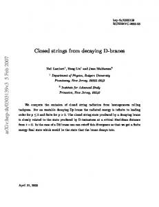
Figure 1: Intersecting (±p, 1)-strings. Arrows denote the orientation of the (solid) D-strings as well as the directions of the (dashed) fundamental string fluxes (the electric fluxes on the D-strings).
where a and p are positive constant parameters, and x ≡ x1 . Since the field Y measures the transverse displacement of the D-strings, when a = 0 we can interpret the geometry of this configuration as a pair of intersecting D-strings with slopes ±p = ± tan(θ/2)
(2.6)
where θ (0 ≤ θ ≤ π) is the angle between the two D-strings (See Fig. 1). Since only diagonal entries are turned on in this case, the solution is basically given by two independent solutions of the abelian system. From the relation (2.3) we see that the electric flux on the two D-strings is given by F 01 = ±px/2πα′ . Thus, the first part of the solution is a (p, 1)-string which is tilted as Y = px, while the second part is a (−p, 1)-string tilted as Y = −px. Since these two satisfy the same BPS equation 2πα′ F01 + ∂1 Y = 0, the brane configuration is supersymmetric. It is known that this kind of supersymmetric intersection admits a deformation which preserves supersymmetry. Such a deformation can be found by producing a “box”-shaped configuration using supersymmetric string junctions [20, 21, 8] (see Fig. 2). Because the parameter a does not violate the BPS condition (2.2), we expect that this parameter should provide an analogous deformation in the Yang-Mills picture. In fact, as shown in [19], turning on this off-diagonal entry in Y produces a recombination of the originally intersecting D-branes (see Fig. 3). It is easy to see that when one diagonalizes the solution (2.5) by use of a gauge transformation one obtains � � p λ(x) 0 , λ(x) ≡ p2 x2 + a2 . Y = (2.7) 0 −λ(x) Thus, it seems that the two D-strings are disconnected for any nonzero value of a. We show in the following subsection by analyzing the D-string charge of the configuration
–4–
Figure 2: Generation of a box. This deformation does not affect the preserved supersymmetries.
that this intuitive picture is correct: the D-strings are indeed localized on the curves pictured in Figure. 3. In the configuration we are considering here, however, the fundamental strings, originally bound in the D-strings, must now stretch from one D-string world-volume to the other, and thus live in the space “between” the branes.
2.2 F-string charge Let us now proceed to study the properties of the supersymmetric solution (2.5). We are particularly interested in understanding the structure of the F-strings running between the disconnected D-strings located at y = ±λ(x). The bulk supergravity currents arising from matrix configurations of multiple D-branes were obtained in [9]. We simply follow the definition given there for the fundamental string current (see also [5, 10, 22]). The source current for the NS-NS y
y
x
x
Figure 3: Intersecting D-strings are recombined when the off-diagonal mode is turned on.
–5–
BM N field is given in our case by � � e 10 (x, k) = TD1 (2πα′ )Str eikY F10 Π � � e 20 (x, k) = TD1 (2πα′ )Str eikY F10 ∂1 Y Π
(2.8)
where k is the momentum along the y direction, and Str is the symmetrized trace, where Y, F , and ∂1 Y are treated as units in the symmetrization.∗ The symmetrized trace which appears in these expressions plays a crucial role in the combinatorics of the current analysis we carry out here and later in the paper. The necessity of using this particular resolution of the ordering ambiguities in the current was found in matrix theory in [23, 24] and was derived from string disk amplitudes in [10]. In ˜ i0 are Fourier transforms of a string charge the expressions (2.8) the components Π density Π0i (x, y) which couples to the B-field through B0i Π0i . The y-dependence of Π0i is defined implicitly through (2.8) through the appearance of the matrix Y in the symmetrized trace; for calculational purposes, we can think of the Fourier transform ˜ as being defined as an infinite sum over multipole moments of Π0i (x, y) in the Π y-direction. We now proceed to evaluate Π10 . Using Y 2 = (p2 x2 + a2 )11, the symmetrized trace is simplified e 10 /TD1 = Π
X (ik)n n
n!
tr [Y n pσ3 ]
X (ik)n (p2 x2 + a2 )(n−1)/2 tr [Y pσ3 ] n! n odd X (ik)n 2p2 x = p λ(x)n/2 2 2 2 p x + a n odd n! � = λ′ (x) eikλ(x) − e−ikλ(x) .
=
(2.9)
Thus, after the Fourier transformation back to the coordinate representation we have Z � � e 10 (x, k) = TD1 λ′ (x) δ(y − λ(x)) − δ(y + λ(x)) .(2.10) Π10 (x, y) = − dk e−iky Π
This shows that this component of the current is non-vanishing only on the location of the D-strings, y = ±λ(x), and can be thought of as an x-component of a string charge density localized to the D-strings. The evaluation of the y-component of the current is a bit more involved. Note that the symmetrized trace gives two cases
∗
tr [Y F01 Y F01 ] = 2p2 (p2 x2 − a2 ) , � � 2 tr Y 2 F01 = 2p2 (p2 x2 + a2 ) .
(2.11)
In most of the relevant literature the gauge A0 = 0 is employed, but here we have used a gauge transformation to derive the currents in the A1 = 0 gauge used here.
–6–
The precise combinatorial factors then give us X (ik)n e 20 (x, k) � � Π 2 = Str Y n F01 (2πα′ )2 TD1 n! n even � � ∞ X (ik)2j 2 2 j j+1 2 2 2 j−1 = (p x + a ) tr Y F01 + Y F01 Y F01 (2πα′ )2 (2j)! 2j + 1 2j + 1 j=0 = 2p2
X (ik)2j p
(2j)!
(p2 x2 + a2 )j − 4a2 p2
X (ik)2j j(p2 x2 + a2 )j−1 (2j + 1)! p
� ∂ X (ik)2j = p2 eikλ(x) + e−ikλ(x) − 4a2 p2 (p2 x2 + a2 )j ∂(a2 ) j (2j + 1)! � � � � 1 ikλ(x) −ikλ(x) 2 ikλ(x) −ikλ(x) 2 2 ∂ e −e +e − 4a p =p e ∂(a2 ) 2ikλ(x) � � � � a2 a2 p2 2 ikλ(x) −ikλ(x) ikλ(x) −ikλ(x) = p 1− e + e + e − e λ(x)2 ikλ(x)3 � 1 � = λ′ (x)2 eikλ(x) + e−ikλ(x) + λ′′ (x) eikλ(x) − e−ikλ(x) . (2.12) ik After the Fourier transform, the current is � � Π20 (x, y) = TD1 λ′ (x)2 δ(y − λ(x)) + δ(y + λ(x)) � � +TD1 λ′′ (x) θ(y + λ(x)) − θ(y − λ(x)) .
(2.13)
Here θ is the step function with
θ(z) =
�
1 (z > 0) 0 (z < 0)
(2.14)
The first term in the current (2.13) is localized on the D-strings as before. The second term, on the other hand, is non-vanishing in the region −λ(x) < y < λ(x). This can be interpreted as indicating that the string flux is flowing from one D-string to another, vertically along y. The distribution of string flux is sketched in Fig. 4. An interesting feature of the y-component of the string current Π20 is that the integral of this flux over y gives a quantity independent of x Z d dy Π20 (x, y) = 2(λ′ (x))2 + 2λ(x)λ′′ (x) = 2 (λ(x)λ′ (x)) (2.15) dx = 2p2 . We have now calculated the full string current density Πi0 (x, y). To check the consistency of this calculation, we can check that this current is conserved, ∂ ∂ Π10 + Π20 = 0 . ∂x ∂y
–7–
(2.16)
y
x
Figure 4: Arrows indicate the directions of the flux current for the fundamental strings. The dashed lines denote the current itself. Note that the vertical dashed lines are actually smeared along x although they look localized in this figure.
This conservation rule follows directly from the preceding expressions. Note that while here we have not included higher-order α′ corrections to the currents, we may expect that such corrections to current conservation automatically cancel since the classical solution of our concern is supersymmetric. Indeed, for similar reasons we expect that our solution also solves the full equations of motion in the nonabelian generalization of Born-Infeld theory; this can easily be checked explicitly to order F 4 , and holds in some situations for the symmetrized trace part of the nonabelian action [25]† (related results in the abelian Born-Infeld theory are discussed in [27]). To see in slightly more detail how the currents are affected by higher-order terms, consider for example the first leading correction to the x-component of the string current [9] �
e 10 (x, k) = TD1 (2πα )Str e Π ′
ikY
� �� 1 1 ′ 2 2 2 F10 1 + (2πα ) F10 − (∂1 Y ) . 2 2
(2.17)
In this expression, the higher-order terms in the parenthesis cancel with each other. Although we have not checked all such higher-order terms (there is no consistent proposal at this time for resolving ordering ambiguities in the higher-order terms in the current), we expect that supersymmetry protects both the solution we have found and its currents. To complete this subsection, we now also evaluate the D-string current of our nonabelian brane configuration. The components of the D-string current are given †
Note that in higher-dimensional configurations, however, the supersymmetry conditions of the Yang-Mills theory may differ from those of the Born-Infeld action [26].
–8–
in Fourier space by � � D1 Ie10 = TD1 Str eikY , � � D1 e 10 . Ie20 = TD1 Str ∂1 Y eikY = Π
A similar computation to the above gives � � D1 I10 (x, y) = TD1 δ(y − λ(x)) + δ(y + λ(x)) , � � D1 I20 (x, y) = TD1 λ′ (x) δ(y − λ(x)) − δ(y + λ(x)) .
(2.18)
(2.19) (2.20)
Again, this current is conserved, and we observe that the D-string charge is located only on the curves y = ±λ(x). This agrees with the eigenvalues of the field Y , as stated in the previous subsection. 2.3 Connection with string junctions We now discuss how the configuration we have constructed is related to the string junctions and networks studied in [6, 7, 8]. In [6], BPS string junctions between three (p, q) di-strings are described as singular string configurations. In the worldvolume theory, such a junction is described by including singular source terms. These singular junctions were combined to form BPS networks of di-strings in [8]. In our construction, we have a completely smooth description of a classical brane system. While the number of D-strings in our system is quantized and finite (2), since we are working in the classical Yang-Mills limit, F-string charge (electric flux) is not quantized. Thus, we should think of our configuration as describing a limiting case of a string network with a large number of fundamental strings connecting two D-strings (see Figure 5). It is interesting to ask how in the quantum theory the quantization of string flux will emerge. Indeed, in the full quantum Born-Infeld theory, we would expect to be able to construct a class of configurations where the F-string and Dstring geometries are equivalent under S-duality (and an exchange of the x − y axes). We discuss this question briefly at the end of this section, and again in Section 4. Let us now check quantitatively that the configuration we have constructed can indeed be interpreted as a continuous limit of a family of networks with many Fstrings. First, consider the local flow of F-string charge along the D-string. As we can see from the asymptotic behaviour of Π10 , the lower D-string loses 2p units of electric flux as x goes from −∞ to +∞. This means that the fundamental strings stuck vertically to the D-strings carry that quantity out from the lower D-string to the upper D-string. This quantity can be evaluated by integrating the second term of Π20 over x, Z dx λ′′ (x) = [λ′ (+∞) − λ′ (−∞)] = 2p . (2.21) This relation follows directly from current conservation, but it also shows explicitly that at each point along the D-string there is essentially a local junction which
–9–
contributes a differential part of the total 2p units of F-string charge. Since the whole configuration is supersymmetric and therefore stable, the tensions of the component strings should be locally balanced. Let us now verify that this is the case. Since the vertical F-strings are smeared along the x direction, the string junctions are correspondingly smeared. Let us concentrate on the distribution around the upper D-string. The F-string current density can be divided into two vectors as ~ ≡ (Π10 , Π20 ) = Π ~ bound δ(y − λ(x)) + Π ~ away (θ(y + λ(x)) − θ(y − λ(x))) ,(2.22) Π ~ bound and Π ~ away are the F-string charge current bound in the upper D-string where Π and away from the D-strings, respectively : ~ bound ≡ TD1 λ′ (x) (1, λ′ (x)) , Π
~ away ≡ TD1 (0, λ′′ (x)) . Π
(2.23)
~ bound is parallel to the upper di-string, the tension of this string at x is given Since Π by p |T~ | = TD1 1 + (λ′ (x))2 . (2.24) This indicates that the tension vector itself is simply given by T~ = TD1 (1, λ′ (x)) .
(2.25)
The difference between the tension vectors at x and x + ∆x is then given by ~ away , T~ (x + ∆x) − T~ (x) = ∆x Π
(2.26)
which is just the tension of the vertical F-string times its density at x times the width ∆x. This shows that the tensions are balanced locally around the D-string.
Figure 5: Intersecting straight di-strings are deformed to recombined di-strings connected by a large number of F-strings. This deformation does not cost any energy and is thus an exactly marginal zero mode of the configuration.
– 10 –
Thus, we have seen that the configuration we have constructed is a smooth limit of a family of string networks with F-strings vertically connecting two D-strings. From (2.15), we see that this configuration is characterized by having a uniform distribution of net string charge in the y-direction. It would be interesting to construct other classical limits of string networks. For example, it seems that it should be possible, at least in the full Born-Infeld theory, to construct string networks, like the brane box configuration, with macroscopic F-string charge localized at certain places on the x-axis. We do not know, however, how to realize such a construction explicitly in the Yang-Mills theory, or if indeed such a construction is possible. 2.4 Other string networks It is straightforward to generalize the preceding construction to a very wide class of string networks. Consider a generic string network with the property that as x → ∞ the set of asymptotic (p, q) strings is the same as that found when x → −∞. We expect that any such network can be constructed using the same general approach used in the preceding discussion. Indeed, we can construct a general set of matrices Y = 2πα′ A0 = x Diag(p1 , p2 , . . . pn ) + C
(2.27)
satisfying (2.2), where pi denotes the slope of the ith D- string (which can be a fraction p/q when q of the pi ’s are identical), Cii give the y-intercepts of the asymptotic (p, q) strings, and the off-diagonal matrix elements Cij parameterize a moduli space of BPS configurations with these asymptotic di-string charges. As an example of this string network construction, consider the configuration x a 0 a 0 a −x a (2.28) Y = 2πα′ A0 = . a 0 a x+1 a 0 a −x + 1 This describes a network of four asymptotic di-strings with slopes p1 = p3 = 1 p2 = p4 = −1 and y-intercepts C11 = C22 = 0 C33 = C44 = 1 . All intersections between strings with opposite slopes are blown up by the same parameter a. Diagonalizing this matrix, we have eigenvalues p √ 1 + σ 1 + 8a2 + 4x2 + 4τ a2 + 4a4 + x2 Yστ = (2.29) 2
– 11 –
-2
3
3
2
2
2
1
1
1
-1
1
2
-2
-1
1
-1
-1
-2
-2
(a) a = 0
3
2
-2
(b) a = 0.1
-1
1
2
-1 -2
(c) a = 0.7
Figure 6: String network of four intersecting branes with various values of the parameter a.
where σ, τ ∈ {±1}. These eigenvalues are graphed for various a in Fig. 6. Just as for the simpler configuration with a single intersection discussed in the previous subsections, the F-string flux for this and other networks can be calculated and shown to give a smooth distribution; as before, this distribution will include a piece which is bound to the D-strings, and a piece which stretches between them, corresponding to a smooth family of string junctions. By using an infinite number of branes, we can construct a periodic string network. Considering the infinite periodic space as the covering space of a torus, we can carry out T-duality on the periodic network [28], giving us a T-dual configuration consisting of D2-branes with momentum encoding the T-dual of the electric flux (string winding). More precisely, consider an infinite brane configuration described by matrices of the form (2.27), where i ∈ Z,
and
pi = (−1)i
(2.30)
i−1 ⌊ 2 ⌋R, i = j Cij = a, i 6= j, i + j ≡ 1 (mod 2) 0, i 6= j, i + j ≡ 0 (mod 2)
(2.31)
This encodes an infinite array of equally spaced di-strings with slopes ±1, with equal parameters describing the deformation of each intersection. Performing a T-duality transformation in the Y direction, we find a configuration of two D2-branes with gauge field � � X 1 x f (y) ′ A0 = Ay = δ(y − 2πR′ n) . (2.32) where f (y) ≡ 2πaR ′ 2πα f (y) −x n Here R′ ≡ 2πα′ /R is the dual radius. This construction gives us a BPS configuration of U(2) Yang-Mills theory on a two-torus, which has two units of D2-brane charge and 2p units of momentum (T-dual to F-string charge in the y-direction). In the gauge we have used here, the
– 12 –
gauge field becomes singular. It would be interesting to study this system further, particularly in the quantum theory. As for our previous examples, this configuration has a momentum distribution which is uniform in the x-direction, but it should in principle be possible to construct periodic configurations analogous to the brane box in Figure 2 which have nonuniform momentum distributions. It would be interesting to understand such configurations better.
3. The ’t Hooft-Polyakov monopole In the previous section we have constructed a family of BPS string networks in classical U(N) Yang-Mills theory. A striking feature of these configurations is that they contain fundamental strings which stretch through a region of space not contained in the D-string world-volume, although the fields on the D-strings are used to construct the Yang-Mills theory. In this section we consider a much more familiar construction: the ’t HooftPolyakov monopole. The Prasad-Sommerfield U(2) monopole [15] is a simple solution of U(2) Yang-Mills theory in 3 + 1 dimensions with a scalar field. In supersymmetric Yang-Mills theory, this configuration is BPS. In [14], a nice geometric picture of this solution was given, wherein the scalar Higgs field is interpreted as describing the shape of a pair of D3-branes connected by a “tube” which shrinks to a point and reverses orientation halfway between the D3-branes. The monopole solution has magnetic flux, corresponding to D-string charge on the D3-branes. We use the nonabelian current analysis method to study where this D-string current lives, and we show that just as for the string networks of the previous section, part of the D-string flux lives on the D3-branes, while another part passes through the space between the branes. 3.1 The BIon Before going to the ’t Hooft-Polyakov monopole, let us first consider a BIon solution corresponding to a BPS abelian monopole; because this configuration exists in the abelian theory, it is much simpler. The BIon solution of the abelian 3+1-dimensional Dirac-Born-Infeld action is [11, 13] 1 −bxi B i = ǫijk Fjk = 3 , 2 r
Φ=
b , r p
(3.1)
which solves the BPS equation Bi = ∂i Φ. Here r ≡ (x1 )2 + (x2 )2 + (x3 )2 , i = 1, 2, 3, and b is a constant which is quantized as b = n/2 where n is an integer [11]. Φ is a transverse scalar which we interpret as a fourth spatial dimension (y), with the rescaling Y = 2πα′Φ. The solution (3.1) is interpreted as a semi-infinite Dstring attached perpendicularly to a D3-brane [11, 13]. Let us compute the D-string charge density for this configuration by use of the current density formula for the
– 13 –
D3-brane. In this case, the general nonabelian formula simplifies as all commutators are dropped, and the D-string charge density is associated with U(1) magnetic flux. We have 2
b ′ ′ e j 0y (k) = TD3 (2πα′)2 Bi ∂i Φeik(2πα )Φ = TD3 (2πα′ )2 4 eik(2πα )b/r . r
(3.2)
So after a Fourier transformation, we obtain j 0y = TD3 (2πα′)2
b2 δ(y − 2πα′b/r) . r4
(3.3)
bxi δ(y − 2πα′b/r) . r3
(3.4)
In the same way, we obtain j 0i = −TD3 (2πα′ )
This shows that the D1-brane current lies completely on the deformed D3-brane surface located at y = 2πα′ b/r (see Fig. 7). Furthermore, it is easy to see that the D-string current is tangent to the D3-branes, and has total flux which integrates at any y to Z d3 x j 0y = 4π(2πα′ )TD3 b = nTD1 . (3.5) Thus, in this abelian case there is no D-string charge “away from” the D3-brane, and there are n units of D-string flux going through a sphere at any finite radius on the D3-brane. y
r Figure 7: A slice of the BIon. The dashed lines with arrows are the D-string charges bound on the D3-brane spike (solid lines).
3.2 The ’t Hooft-Polyakov monopole Let us now consider the ’t Hooft-Polyakov monopole. The BPS equation 1 ǫijk Fjk = Di Φ 2
– 14 –
(3.6)
admits the Prasad-Sommerfield solution [15] Aai = ǫaij (1 − K(r))
Aa0 = 0 ,
Φa = −H(r)
xj , r2
xa , r2
where we have used the SU(2) decomposition Aµ = K(r) = P r/ sinh(P r) ,
P3
a=1
Aaµ (σa /2), and where
H(r) = P r coth(P r) − 1 , for a constant P . The Higgs field Φ can be diagonalized by a gauge transformation as � � 0 P coth(P r) − 1r Φ= . (3.7) 0 −P coth(P r) + 1r After the proper rescaling Y = 2πα′ Φ, the location of the D3-brane is given by y = ±λ(r) ≡ ±πα′
H(r) . r
(3.8)
This corresponds to a simple D3-brane geometry, shown in the solid line of Figure 8. Now let us consider the D-string flux in this configuration. Before explicitly computing this flux, we can note that since the monopole solution is smooth at r = 0 we cannot have the full flux living on the brane, since this would entail a finite flux passing through the vanishing “neck” of the tube connecting the branes. Thus, we see qualitatively that some part of the D-string flux must move off the D3-brane world-volume. More explicitly, we have � � � � 1 H(1 − K) 1 H xi HK 1 Di Φ = ǫijk Fjk = − ∂r + x σ − σi . (3.9) a a 2 r r2 r3 2 r2 2 The components of the D-string current density are given by � � 1 ′ )Φ 0y ′ 2 ik(2πα e j = (2πα ) TD3 Str (ǫabc Fab Dc Φ)e , 2 � � 1 ik(2πα′ )Φ 0a ′ e . j = 2πα TD3 Str ǫabc Fbc e 2
(3.10)
A straightforward calculation similar to the previous section gives the following result � 1 0y ′ 2 j = (2πα ) TD3 (1−K 2 )2 (δ(y − λ) + δ(y + λ)) (3.11) 4r 4 � HK 2 (θ(y + λ) − θ(y − λ)) , + 2πα′r 3 xa (3.12) j 0a = (2πα′)TD3 3 (1 − K 2 ) (δ(y − λ) − δ(y + λ)) . 2r
– 15 –
It is easy to check that this current density satisfies the current conservation law, ∂y j 0y + ∂a j 0a = 0 .
(3.13)
The meaning of the terms in the current density expression (3.11) and (3.12) is obvious, analogous to the previous section: the current (3.12) and the first term in (3.11) describes the D-string charge density bound on the D3-brane world-volume surfaces, while the second term in (3.11) describes straight D-strings connecting the upper and lower D3-branes, away from the D3-brane surface. This feature is analogous to the F-string current density observed in the previous section. y
r
Figure 8: D-string current distribution (dashed lines) of the ’t Hooft-Polyakov monopole.
For large r, these current expressions coincide with the BIon case, and one can see that the second term in (3.11) damps exponentially. On the other hand, for small r, the first term in (3.11) converges to a constant while the second term apparently diverges, as � 4 � P P2 0y ′ 2 j ∼ (2πα ) TD3 (δ(y − λ) + δ(y + λ)) + (θ(y + λ) − θ(y − λ)) (3.14) . 36 6πα′r This is still consistent with the comment above regarding the lack of a singularity in F at the “neck” r = 0. The second term in j 0y goes as 1/r. Although this component of the current is unbounded as r → 0, however, since the distance between the branes goes as r in this limit, all multipole moments of the current are finite. We have now seen that the shape of the D3-branes in the monopole configuration must be affected by the D-strings stretching vertically between the branes. As in Section 2, it should be possible to verify that the tension of the D-strings precisely produces the correct amount of curvature of the D3-brane world-volume in the monopole configuration. Indeed, based on a qualitative argument of this kind,
– 16 –
the existence of this D-string distribution away from the D3-brane surface was conjectured in [25]. In Refs. [29, 25, 30, 31], classical solutions of SU(N) Yang-Mills theories corresponding to string junctions ending on parallel D3-branes [32] (1/4 BPS dyons) were constructed. These constructions give natural generalizations of the ’t Hooft-Polyakov monopole and the Julia-Zee dyon. In [25], the shape of the deformed D3-brane surface in this 1/4 BPS dyon was studied in detail, and it was observed that in fact (p, q)-strings away from the deformed D3-brane surfaces are necessary to consistently interpret the curved trajectories of the D3-branes. In this paper we have demonstrated that these strings are actually existent, for the simplest case of the ’t Hooft-Polyakov monopole. We expect that a similar computation of the NS-NS and R-R current densities in the general 1/4 BPS dyon case will confirm the more general conjecture in [25].
4. Strings in the vacuum from Yang-Mills tachyons As an application of the methods developed in the previous part of this paper, we now show how strings and D-strings in the vacuum appear in Yang-Mills theory after tachyon condensation on a system of intersecting branes. Sen’s conjectures on tachyon condensation [16] in brane-antibrane systems have led to many interesting developments in recent years. In particular, these conjectures have led to a new wave of development of string field theory, and to new efforts to understand time-dependent processes in string theory. In the context of braneantibrane annihilation in type II superstring theory, Sen’s conjectures essentially make three assertions: 1. Condensation of the tachyon in a brane-antibrane system describes the annihilation of the D-branes to the true vacuum. 2. All open string degrees of freedom are gone in the true vacuum, although closed strings and infinitely extended open strings still appear as degrees of freedom. 3. Lower-dimensional D-branes appear as solitons of the tachyon field. In particular, vortex-like topological defects of the tachyon field correspond to stable BPS D-branes with codimension two. We will be interested here in parts 2 and 3 of these conjectures. A system containing a brane and an antibrane cannot be described in Yang-Mills language, as there is no static gauge with respect to which both the brane and antibrane have the same orientation. It is, however, possible to consider a pair of branes at an arbitrary angle θ < π in Yang-Mills theory, just as we did for D-strings in Section 2. In the absence of supersymmetry-saturating fluxes, such a pair of intersecting D-branes has a tachyon in the spectrum [33]. The condensation of this tachyon is
– 17 –
closely related to the condensation of a brane-antibrane tachyon, and gives rise to a dynamic recombination of the branes, leaving a true vacuum in a region around the initial brane intersection locus. This recombination can be described in Yang-Mills language [17, 18, 19], and has been recently used in models of cosmology [34]. In this section we use the Yang-Mills description of a pair of intersecting branes to give a qualitative picture of how fundamental strings and codimension two D-branes appear in the vacuum according to conjectures 2 and 3 above. The question of how closed or infinitely extended fundamental strings appear in the stable vacuum after tachyon condensation has sparked quite a bit of recent work. In particular, it was argued in [35, 36, 37] that near the stable vacuum an effective gauge theory for the brane system describes fundamental strings as confined tubes of electric flux. In this section we consider a pair of intersecting branes in the presence of an electric flux. We show that when the tachyon condenses, the electric flux is converted into open strings stretching through the vacuum between the recombined D-branes. We use the nonabelian current analysis methods from the previous sections to show that the resulting strings indeed stretch between the branes. This gives a qualitative picture of how fundamental strings in the vacuum appear in Yang-Mills theory. To study the third of Sen’s conjectures, we perform a similar analysis. We turn on a vortex-shaped tachyonic fluctuation of the Yang-Mills field on a D3-brane and compute the D-brane currents in a similar way. This shows how codimension two D-branes stretch between the recombined D-branes. In subsection 4.1 we review the Yang-Mills description of the recombination of intersecting branes through tachyon condensation. In subsection 4.2 we describe how fundamental strings stretching between the recombined branes arise from an initial electric field. In subsection 4.3 we show how a vortex tachyon configuration gives rise to D-strings stretching between recombined D3-branes. 4.1 Sen’s conjecture and recombination We begin by reviewing how the recombination process of a pair of intersecting Dbranes can be described in Yang-Mills theory. This was studied in a T-dual picture on the torus in [17] and for branes in infinite flat space in [18, 19]. Most of this discussion follows the analysis of [19]. Let us consider two D-strings for simplicity. The low-energy effective description of parallel D-strings is given, as in Section 2, by the 1+1 dimensional SU(2) super Yang-Mills action (2.1). We decompose the matrix fields as Aµ = Aaµ (σa /2) where a = 1, 2, 3 and σa are the sigma matrices. The location of the D-strings is specified by the eigenvalues of the transverse scalar field Y , which is related to the usual Higgs field as 2πα′ Φa ≡ Y a . The (unstable) classical solution representing the intersecting D-strings is Φ3 = qx ,
Aµ = 0 ,
– 18 –
(4.1)
where the linear coefficient q is the slope of the D-strings, q=
1 tan(θ/2) (> 0) . πα′
(4.2)
We have introduced the intersection angle θ, which with θ = 0 corresponds to a parallel pair of D-strings (which is BPS) while θ = π represents an anti-parallel pair of D-strings (parallel brane-antibrane). The analysis of the spectrum of fluctuations of this system shows that there are two tachyonic fluctuation modes, � � � � qx2 qx2 2 1 (2) 1 2 (1) , Φ (x) = −Ax (x) = C (t) exp − (4.3) , Φ (x) = Ax (x) = C (t) exp − 2 2 with the mass squared m2 = −q appearing in the free field equation for the fluctuation modes, (∂02 − q)C (i) (t) = 0. For small θ, this mass squared m2 = −q was found to be identical to that of the string worldsheet spectrum given in [33]. Turning on the tachyon fields (4.3) gives rise to a recombination of the intersecting D-strings [19]. In fact, when only these modes are turned on, the eigenvalues of the field Y are given by p y = ±πα′ q 2 x2 + C 2 e−qx2 , (4.4)
where C 2 = (C (1) )2 + (C (2) )2 . The shape of the associated D-strings is shown in Fig. 9. Here we have diagonalized the scalar field directly, but, as in Section 2, if we plug the configuration with the tachyon turned on into the D-string current formula (2.18), we obtain the same result. In this section of this paper we use Yang-Mills theory to study the brane structure of field configurations analogous to (4.4) when fundamental strings or codimension two D-branes are included in the D-brane configuration through the addition of electric fields or a topologically stabilized vortex configuration of the tachyon. The Yang-Mills action is only the leading part of the full brane action, which is given by a nonabelian analogue of Born-Infeld theory (which is not currently fully known). The Yang-Mills description is accurate at leading order in θ, when the field strength 2πα′ F and θ are of comparable order and are both small compared to 1. While we expect that the form of the tachyon modes (4.3) will be essentially the same in BornInfeld theory, the formula for the mass should have tan(θ/2) → θ/2 [33, 17, 19, 38]. Even at finite θ, however, we expect that the Yang-Mills action should give a good qualitative description of the physics of the tachyonic mode. Thus, at a qualitative level, we can consider what happens as θ is of order unity. When the angle θ is π, the intersecting D-strings become a parallel D-string and anti-D-string. At this angle, we can no longer choose static gauge along the x-coordinate, and we must instead parameterize the world-volume of the D-strings by the static coordinate y. At the point θ = π, we cannot use Yang-Mills theory to describe the system, but we expect that qualitative features of brane-antibrane
– 19 –
annihilation should be captured in the Yang-Mills description of the theory in the limit θ → π. Let us view the intersecting D-strings (at θ < π) from the point of view of the D-brane world-sheet parameter y. As seen in Fig. 9, when the tachyon mode is turned on, a part of the “world-volume” parameterized along the y direction disappears due to the recombination, that is, the local annihilation of the brane and the antibrane. In this sense, the Yang-Mills analysis we carry out here provides an interesting realization of brane-antibrane annihilation. y
y
x
x
Figure 9: D-strings are recombined. By rotating these figures by π/2, one can see the local brane-antibrane annihilation occurring around the origin.
At any angle θ, the dynamical process of D-brane recombination is very complicated. A full treatment of this process would require string field theory or the full nonabelian Born-Infeld action. Even in the simplified Yang-Mills action, this process is very complicated since all string modes become involved after an infinitesimal time. Nonetheless, when we consider very short time scales, only the tachyon mode itself will be excited. Thus, at short times, to understand the geometry of the D-brane configuration just after recombination has occurred, it will suffice to consider configurations where only the tachyon field has been turned on, and where this field has a very small coefficient C. This is the spirit in which the following analysis should be taken: the analysis is only technically accurate at very small θ and at very small time. Nonetheless, we believe that it gives interesting insight into the way in which strings and branes appear in the vacuum produced by tachyon condensation. 4.2 Fundamental strings after tachyon condensation 4.2.1 Correspondence to Yang-Mills theory In the usual language of the brane-antibrane near θ = π, we have two gauge fields: A(+) and A(−) . These are linear combinations (+ and −) of two U(1) gauge fields
– 20 –
living on the brane and the antibrane. When the tachyon condenses, the field A(−) is Higgsed, since the tachyon is charged under the gauge group relevant for this gauge field. It has been conjectured that the field A(+) is confined and gives rise to fundamental strings when the original unstable brane-antibrane pair disappears after the tachyon condenses [35, 36, 37]. In the Yang-Mills description of intersecting D-strings, we also have two U(1) gauge groups which are unbroken by the intersecting D-brane solution. This is consistent with the above observation; these two descriptions are just related by changing the direction of the world-volume parameterization. In the Yang-Mills description, one U(1) gauge field is the σ3 component of the full SU(2) gauge field. The other U(1) is the overall trace U(1), which decouples completely from the SU(2) sector. To proceed, we have to check which U(1) in the Yang-Mills theory corresponds to A(+) . One may naively think that the latter, trace, U(1) should correspond to A(+) , but this is not the case. In changing the world-volume parameterization from the horizontal direction x (Yang-Mills description) to the vertical direction y (braneantibrane description), we must use the (leading-order) relation AYM = x
∂Y brane−antibrane A . ∂x y
(4.5)
Noting that the background (4.1) gives ∂Y /∂x ∼ σ3 , this relation shows that the (+) Chan-Paton (CP) factor of the Yang-Mills field corresponding to Ay (whose CP factor is 112×2 ) becomes in the brane-antibrane system σ3 = σ3 · 112×2 , (−)
while for Ax
(4.6)
(whose CP factor is σ3 ), one has 112×2 = σ3 · σ3 .
(4.7)
In effect, the CP factors 112×2 and σ3 in the two descriptions are exchanged, and so we obtain the following correspondence: Brane-antibrane (y direction) Yang-Mills (x direction)
A(+) σ3
A(−) 112×2
4.2.2 Fundamental strings and electric fields in A(+) Let us first consider the field A(+) . This field contains the most interesting physics; it has been conjectured to be confined and to provide fundamental strings after the tachyon has condensed. From the correspondence above, we know that the corresponding field in the Yang-Mills theory is the σ3 component of the SU(2) gauge field. In fact, we have already analyzed the effects of including an electric field in this σ3 sector in Section 2. Although there we considered only the special case where the field took the precise value needed to preserve the supersymmetries of the system,
– 21 –
the analysis of Section 2 already captures the intrinsic features of the phenomena we are interested in. More precisely, let us consider modifying the intersecting brane configuration (4.1) by including a small electric field A0 = ǫxσ3 .
(4.8)
As long as ǫ ≪ q, the inclusion of this field will not change the dominant form of the tachyonic fluctuation modes (4.3). Then, turning on the tachyon mode C (1) will give a configuration which for small x takes the form � � � � � � 1 0 C 1 qx C ǫx 0 , A1 = , A0 = . (4.9) Φ= 0 −ǫx 2 C qx 2 C 0 For small x, we may discard the off-diagonal components in F10 , which are proportional to x, while the diagonal components are constant. Since F10 appears linearly in each component of the F-string current density (2.8), the F-string current in this configuration is proportional to that computed in Section 2, and is given by multiplying the current components (2.10, 2.13) by the overall factor 2πα′ǫ/p, where we take p → πα′ q and a → πα′ C. This fundamental string distribution is depicted in Figure 4. Thus, as in the supersymmetric case discussed in Section 2, we find that after tachyon condensation an electric flux on intersecting branes is converted into fundamental strings which extend through the region of space between the newly disconnected branes. This gives a very satisfying picture in Yang-Mills theory of how Sen’s second conjecture is realized. Even in the Yang-Mills approximation, it seems, fundamental strings stretching through the vacuum can be seen in the region of space where brane-antibrane annihilation has occurred. We expect that qualitatively similar results should hold in the full Born-Infeld theory and in string field theory. It should be reemphasized that this picture of strings in the vacuum is fundamentally different than other pictures like the spike solution of [11, 13], where F-strings stuck vertically onto a D-brane world volume are realized as an electric flux on a cylindrically deformed Dp-brane world-volume whose spatial configuration has a topology R × S p−1 . In that picture, the fundamental string is taken to appear in the limit where the radius of the S p−1 vanishes. In the context of tachyon condensation, this realization of the F-strings (or more precisely, a bound state of F-strings and D-branes) was recently used as a possible description of fundamental strings after tachyon condensation [39, 40, 41]. On the other hand, what we have found here is truly a representation of the F-strings “away from” the D-branes. The picture we have found here seems to be much more natural from the point of view of Sen’s conjectures, where we expect the fundamental strings to exist in a region of space-time completely devoid of D-brane matter.
– 22 –
One feature of the fundamental strings which is not as clear from this picture, however, is the confinement mechanism of the strings. As discussed in Section 2, the classical configurations we have found have F-string charge which is smeared in the xdirection. In the classical theory, fundamental string charge is not quantized, so as for the supersymmetric configurations discussed in Section 2, we expect that a quantum treatment will be needed to fully understand the confinement and quantization of fundamental strings in this Yang-Mills model. 4.2.3 Electric field in A(−) An electric flux for A(−) corresponds to a Yang-Mills background � � ′ qx 0 A0 = 0 q′x
(4.10)
in addition to the original configuration (4.1), with some constant q ′ . This additional field is in the overall U(1) sector, so there is no influence on the fluctuation analysis. This means that there are still the same tachyonic fluctuation modes as in (4.3), and after the tachyon condensation the D-strings are recombined.
Figure 10: Recombination of intersecting D-strings with A(−) electric flux. The solid lines represent the D-strings, while the dashed lines represent Fstrings. Note that the asymptotic orientations of the bound F-strings are different from those in section 4.2.2, where the strings had to stretch between the separated branes.
Let us see what happens to the F-string charge density. The charge density formulae are given in (2.8), and we substitute the configuration (4.1, 4.10) with tachyon condensation C 6= 0 into (2.8). Now, since our electric field is in the overall U(1) sector, F10 in the formula (2.8) does not contribute to the computation except as an overall constant factor, and as a result the F-string charge density (2.8) is simply proportional to the D-string charge density (2.18). Since we know that the D-strings are recombined, then this shows that the F-strings are also recombined, and so there remains no F-string connecting the recombined D-strings (see Fig. 10).
– 23 –
This contrasts with the above results for the gauge field A(+) , and is consistent with the brane-antibrane picture in which the gauge field A(−) is Higgsed after tachyon condensation. 4.3 Descent relation in Yang-Mills theory Let us now turn our attention to the third conjecture, describing the creation of lower-dimensional D-branes as tachyonic topological defects on unstable D-branes. In this subsection we consider the formation of a vortex-like tachyon which gives a codimension two BPS D-brane in the brane-antibrane system. We will specialize in particular to the formation of D-strings connecting intersecting D3-branes which recombine through tachyon condensation. We see again that the charge of the lower dimensional D-brane lies “off” the recombined D3-brane world-volume. The resulting charge distribution is quite similar to that of the ’t Hooft-Polyakov monopole analyzed in the previous section. 4.3.1 Vortex formation To consider vortex formation in the tachyon system, we first must check that the tachyonic modes (4.3) found in the Yang-Mills theory of intersecting D-branes actually have nontrivial topology in their vacuum manifold. In fact, a gauge transformation with a transformation parameter proportional to σ3 rotates one of these fluctuations into the other, so the tachyon potential has a U(1) symmetry and is written only in terms of the modulus of the complex tachyon fluctuation, |C (1) + iC (2) |. Hence, we expect a vortex tachyon which is topologically stable. This is consistent with the fact that the brane-antibrane setup has the same structure and our intersecting brane setup is continuously related to it. In this subsection we generalize the intersecting brane configuration from Dstrings to D3-branes so that we may have a tachyon vortex in the (2 + 1)-dimensional intersection submanifold. The D3-brane world-volumes are parameterized by the coordinates (t, x1 , x2 , x3 ), and the intersection submanifold is parameterized by (t, x2 , x3 ). The coordinate x1 plays the role of the world-volume coordinate x in the intersecting D-string case. Taking the coefficients of the tachyon modes (4.3) along x1 to be functions of the remaining coordinates t, x2 , x3 , we have the equation of motion [(∂t )2 − (∂2 )2 − (∂3 )2 + m20 ] C (i) (t, x2 , x3 ) = 0
(4.11)
where negative m20 = −q is the tachyon mass squared.‡ Since we have generalized the configuration (4.1) trivially to the D3-brane intersection, a homogeneous tachyon condensation (non-zero C) generates the recombination shown in Fig. 11. ‡
Of course since we have more gauge fields on the world volume, the fluctuation analysis should be examined again in this case. It turns out, however, that the tachyonic fluctuations still take the form (4.3) in the intersecting D3-brane case, although the profiles of the higher massive modes are corrected.
– 24 –
y
y
x1
x1
x2 , x3
x2 , x3
Figure 11: The intersecting D3-branes are recombined by the tachyon condensation which is homogeneous along the intersection submanifold.
Next we turn on a vortex-shaped tachyon, C (1) = cx2 ,
C (2) = cx3 ,
(4.12)
where c is a constant.§ The linear profile (4.12) is valid only for small x2 and x3 . As mentioned above, the tachyonic fluctuations parameterize S 1 and so it is clear from the asymptotic form that the mode (4.12) corresponds to the formation of a tachyon vortex, which should give a codimension two D-brane. What we would now like to see is precisely how this Yang-Mills configuration, together with the original background (4.1), produces a lower-dimensional D-brane charge. Let us consider what kind of D-brane configuration is expected in the present case from Sen’s conjecture. Firstly, at θ = π the brane configuration is a parallel D3-brane-anti-D3-brane pair along y, so after the tachyon condensation of the vortex in the x2 -x3 world-volume space, the topological defect is identified with a D-string which is orthogonal to the x2 and x3 directions. This means that the D-string should be oriented along the y axis. Secondly, we know from the preceding discussion that the tachyon condensation on the intersecting D3-branes realizes the usual D3-brane recombination. Hence, combining these predictions, we expect that condensation of §
To be precise, this vortex-shaped tachyon represents an unstable direction which will grow exponentially through the equation of motion. If we solve the fluctuation equation (4.11), we may obtain a time-independent solution for this unstable mode √ √ C (1) = (c/ q) sin qx2 ,
√ √ C (2) = (c/ q) sin qx3 ,
(4.13)
where c is a constant. This represents a periodic array of D-strings whose periodicity is tuned to give a marginal direction of deformation. We can expand this expression for small x2 and x3 and obtain the vortex configuration (4.12). It is obvious from this expression that the lower dimensional D-branes are created as infinite pairs of brane-antibranes so that the total Ramond-Ramond (RR) charge is preserved. In general, the functions C (i) are time-dependent and describe dynamical creation and annihilation of the lower dimensional D-branes.
– 25 –
the tachyon vortex (4.12) will lead to a configuration containing a D-string stretched between two recombined D3-branes. We will now see that this is indeed the case, by computing the location of the generated D-string charges. The D-strings are again found to live away from the deformed D3-brane world-volume surface, just like the fundamental strings discussed above and like the D-strings in the ’t Hooft-Polyakov monopole analyzed in the previous section. 4.3.2 Shape of the D3-brane Once the vortex is given as (4.12), it is possible to study the shape of the D3-brane world volume. The total scalar field configuration is 2
2
Y = πα′(qx1 σ3 + cx2 e−q(x1 ) σ1 + cx3 e−q(x1 ) σ2 ) .
(4.14)
The eigenvalues of this matrix, which give the location of the D3-brane world-volume, are then given by q ′ y = ±λ(x1 , x2 , x3 ) ≡ ±πα q 2 (x1 )2 + c2 e−2q(x1 )2 ((x2 )2 + (x3 )2 ) , (4.15) where y is the bulk coordinate corresponding to the field Y . This immediately shows that at the vortex core x2 = x3 = 0 the intersecting D3-branes still touch each other, while away from the origin those are disconnected (recombined), as seen in Fig. 12. This is similar to the D3-brane deformation in the ’t Hooft-Polyakov monopole [14] discussed in the previous section. y
y
x1
x1
x2 , x3
x2 , x3
Figure 12: Plot of y = ±λ(x1 , x2 , x3 ) after intersecting D3-branes are recombined by a vortex-like tachyon.
4.3.3 Generation of D1-brane charge In this subsection we explicitly compute the D-string RR charge density produced by this Yang-Mills field configuration. From the RR couplings in the D3-brane effective field theory, the relevant components j 0a of the charge density are again given by
– 26 –
(3.10). Let us first evaluate j 0y . Since again in this case (Φ)2 = Y 2 /(2πα′)2 is proportional to the unit matrix, � 1� 2 λ2 2 (Φ)2 = q (x1 )2 + c2 e−2q(x1 ) ((x2 )2 + (x3 )2 ) 112×2 = 112×2 , (4.16) 4 (2πα′ )2 the computation of the density current can be performed in the by-now familiar fashion. The field strengths are given by F23 = 0,
2
F12 = D3 Φ = ce−q(x1 ) σ2 /2,
2
F31 = D2 Φ = ce−q(x1 ) σ1 /2 .
(4.17)
Then using the results 2
tr [σ1 Φσ1 Φ] = (−q 2 (x1 )2 + c2 e−2q(x1 ) ((x2 )2 − (x3 )2 ))/2 , 2
2
2 −2q(x1 )2
tr [σ1 σ1 ΦΦ] = (q (x1 ) + c e
2
2
(4.18)
((x2 ) + (x3 ) ))/2 ,
(4.19)
)2
(4.20)
tr [σ2 Φσ2 Φ] = (−q 2 (x1 )2 + c2 e−2q(x1 (−(x2 )2 + (x3 )2 ))/2 , )2
tr [σ2 σ2 ΦΦ] = (q 2 (x1 )2 + c2 e−2q(x1 ((x2 )2 + (x3 )2 ))/2 ,
(4.21)
we obtain h i ′ ′ 2 e j 0y = TD3 (2πα′)2 Str σ1 σ1 eik(2πα )Φ + σ2 σ2 eik(2πα )Φ c2 e−2q(x1 ) � 2 ′ 2 2 2 ′ 2 2 −2q(x1 )2 λ − (πα ) q (x1 ) (eikλ + e−ikλ ) = TD3 (πα ) c e λ2 � λ2 + (πα′ )2 q 2 (x1 )2 ikλ −ikλ (e − e ) . (4.22) + ikλ3 After a Fourier transformation, we have � 2 ′ 2 2 2 0y ′ 2 2 −2q(x1 )2 λ − (πα ) q (x1 ) j = TD3 (πα ) c e (δ(y − λ) + δ(y + λ)) λ2 � λ2 + (πα′ )2 q 2 (x1 )2 (θ(y + λ) + θ(y − λ)) . (4.23) + λ3 This D-string charge density exhibits a by-now familiar structure. The first term describes D-strings running along the deformed D3-brane surface y = ±λ(x1 , x2 , x3 ). The second term describes vertical D-strings connecting the upper and the lower D3branes. These D-strings lie off the world-volume of the D3-branes, and are closely analogous to the D-strings found in the ’t Hooft-Polyakov monopole in the previous section. It is easy to evaluate the other components of the D-string current as j 01 = 0 , 2
j
02
j 03
c2 e−2q(x1 ) (δ(y − λ) − δ(y + λ)) , = πα TD3 x2 λ 2 c2 e−2q(x1 ) = πα′ TD3 x3 (δ(y − λ) − δ(y + λ)) . λ ′
– 27 –
(4.24)
y
x1 x2 , x3
Figure 13: A schematic view of the distribution of the D-string charge density (dashed lines) after tachyon condensation. Here we describe only the part of the D-string current which is away from the D3-brane surface (solid surface). The arrows denote the directions of the D-string charge density.
y
x3
Figure 14: The distribution of the D-string charge density (dashed lines) in the slice x1 = x2 = 0. Here again, the vertical dashed lines should be understood as the ones which are smeared along the horizontal direction. The arrows denote the directions of the D-strings. Solid lines denote slices of the D3-branes.
One can verify that the current conservation law (3.13) is satisfied as a consistency check.¶ As expected, the components (4.24) of the D-string current do not describe any D-strings located away from the D3-branes, but give only D-string charges along the D3-brane surface. Fig. 13 shows schematically how the D-string charges are distributed in the bulk. In Figure 14, the D-string charge density is shown in the spatial slice x1 = x2 = 0. ¶
This current conservation holds even though the configuration we are considering is not static, since the current j µν is antisymmetric in its indices and the conservation law for the charge density µ = 0 does not involve any time derivative.
– 28 –
We have thus shown that D1-branes suspended between recombined D3-branes appear as a result of the formation of a vortex-like tachyon on an intersecting pair of D3-branes. This gives a simple Yang-Mills description of how Sen’s third conjecture on the formation of lower-dimensional D-branes through topological tachyon defects is realized in the case of the intersecting D-branes. In this situation, as in the description of fundamental strings in the previous subsection, several caveats apply. In particular, the analysis we have carried out here is only valid for short times and small values of x near the core of the vortex. Note, however, that unlike in the case of fundamental strings, the quantization of D-string charge is already seen in the classical picture presented here, as this quantization arises simply from the quantization of the first Chern class in the nonabelian gauge theory.
5. Conclusions and discussion In this paper we have analyzed a number of nonabelian D-brane configurations containing fundamental strings and lower-dimensional D-branes. We used the nonabelian formulae for the fundamental string and D-brane currents from [9] to compute the spatial distribution of string and D-brane charges. We found that in a variety of situations, these charges extend through regions of space away from the D-branes on which the original nonabelian theory was defined. This phenomena was demonstrated for string networks in (1+1)-dimensional nonabelian Yang-Mills theory, for the ’t Hooft-Polyakov monopole in (3+1)-dimensional Yang-Mills theory, and for tachyonic intersecting brane configurations, where we found F-strings and D-strings in the vacuum formed in the brane annihilation process. The constructions we have presented here give an interesting new way in which D-brane field theory encodes the geometry of transverse directions of space-time. In Section 2 we constructed a new class of supersymmetric solutions of the nonabelian Yang-Mills equations of motion. These solutions correspond geometrically to D-strings with fundamental strings stretching between them, and give a smooth description in Yang-Mills theory of string networks. By performing the nonabelian analysis of the current density, we showed that the fundamental string charge density has support in regions of space-time away from the world-volume of the D1-branes on which the Yang-Mills degrees of freedom live. There are a number of interesting open questions related to these Yang-Mills string networks. In particular, we do not know how to construct networks where the total F-string charge in the vertical (Higgs) direction is inhomogeneous in the spatial Yang-Mills coordinate, or even whether such configurations can be constructed. The Ansatz we used to solve the BPS equation (2.2) is fairly restrictive; it is possible that a more general family of solutions may be found by loosening the constraints imposed by this Ansatz. All the analyses we performed here were restricted to the Yang-Mills approximation. This is a good approximation for systems of D-branes when the gauge field and
– 29 –
transverse fluctuations are small, and gives a qualitative picture of many important aspects of the physics of D-branes. In particular, we described particular limits in which the picture of fundamental strings and D-strings in the vacuum arising from tachyon condensation is valid. For a full understanding of string physics, however, it is necessary to extend the analysis to a more complete formalism such as string field theory or nonabelian Born-Infeld theory (which, when derivative corrections are included, should describe all the physics of string field theory). Because they are protected by supersymmetry, we expect that the supersymmetric nonabelian brane configurations we have considered in Sections 2 and 3 should still be valid in the full theory when α′ corrections are included. Another interesting question is how the configurations we have constructed here behave under S-duality. In general, we only expect S-duality to hold at the quantum level. For example, the quantization of fundamental strings in the string networks considered in Section 2 only arises in the quantum theory. While we expect that there are string networks like the box configuration shown in Figure 2 which are invariant under S-duality and an exchange of the x and y coordinates, this is probably not possible to see in the classical theory. On the other hand, some aspects of Sduality may be visible even classically. This is well-understood in the abelian theory, where S-duality is equivalent to Hodge duality on the field strength, but is not well understood in the supersymmetric theory. If one performs an S-duality on the configuration of Fig. 1, after performing T-duality along the transverse directions x2 and x3 , one finds a brane configuration in which D-strings and F-strings are replaced by D3-branes and smeared D-strings respectively. A Yang-Mills representation of such a configuration is known [42]; in this construction an off-diagonal zero mode is present, which is similar to our deformation parameter a. It would be interesting to investigate further these nontrivial classical configurations which seem to be S-dual to each other. There is a close connection between the nonabelian currents we have used in this paper and the Seiberg-Witten map [47], which relates noncommutative YangMills theory to Born-Infeld theory. The D-brane multipole currents used here were applied in [43, 44, 45, 46] to obtain an explicit expression for the Seiberg-Witten map. Computing the Seiberg-Witten map for given matrix (∼ noncommutative) field configurations is equivalent to finding the RR current densities j 0i for these configurations. For example, in [48] the Seiberg-Witten map of fluxons [49, 50, 51, 52] showed tilted D-string configurations [53, 54] specific to noncommutative monopoles [53, 55, 56], while a perturbative version of this phenomena has been observed in [57]. It would be interesting to compute other components such as j 0y in these configurations to confirm this brane interpretation. In this paper we have restricted attention only to the leading short-time behavior of the intersecting brane tachyon. The full time-dependent tachyon condensation process may have interesting applications to brane cosmology [34]. It would be
– 30 –
interesting to investigate possible applications of the methods developed in this paper to intersecting brane cosmological models.
Acknowledgments We would like to thank H. Ooguri, A. Sen, D. Tong, J. Troost, and M. Van Raamsdonk for helpful discussions and comments. K. H. is grateful to the CTP at MIT for kind hospitality, where a part of this work was done. This work was supported in part by the Grant-in-Aid for Scientific Research (No. 12440060, 13135205 and 15740143) from the Japan Ministry of Education, Science and Culture and in part by the DOE through contract #DE-FC02-94ER40818.
References [1] R. G. Leigh, “Dirac-Born-Infeld Action from Dirichlet σ-Model”, Mod. Phys. Lett. A4 (1989) 2767. [2] J. Polchinski, “TASI Lectures on D-branes”, hep-th/9611050. [3] E. Witten, “Bound States of Strings and p-Branes”, Nucl. Phys. B460 (1996) 335, hep-th/9510135. [4] W. Taylor, “Lectures on D-branes, Gauge Theory and M(atrices),” hep-th/9801182. [5] R. C. Myers, “Dielectric-Branes,” JHEP 9912 (1999) 022, hep-th/9910053. [6] K. Dasgupta and S. Mukhi, “BPS Nature of 3-String Junctions,” Phys. Lett. B423 (1998) 261, hep-th/9711094. [7] J. P. Gauntlett, J. Gomis and P. K. Townsend, “BPS Bounds for Worldvolume Branes,” JHEP 9801 (1998) 003, hep-th/9711205. [8] A. Sen, “String Network,” JHEP 9803 (1998) 005, hep-th/9711130. [9] W. Taylor and M. van Raamsdonk, “Multiple Dp-branes in Weak Background Fields, Nucl. Phys. B573 (2000) 703, hep-th/9910052; “Multiple D0-branes in Weakly Curved Backgrounds,” Nucl. Phys. B558 (1999) 63, hep-th/9904095. [10] Y. Okawa and H. Ooguri, “Energy-momentum Tensors in Matrix Theory and in Noncommutative Gauge Theories,” hep-th/0103124. [11] C. G. Callan, Jr. and J. M. Maldacena, “Brane Dynamics From the Born-Infeld Action,” Nucl. Phys. B513 (1998) 198, hep-th/9708147. [12] P. S. Howe, N. D. Lambert and P. C. West, “The Self-Dual String Soliton”, Nucl. Phys. B 515, 203 (1998), hep-th/9709014.
– 31 –
[13] G. W. Gibbons, “Born-Infeld Particles and Dirichlet p-branes,” Nucl. Phys. B514 (1998) 603, hep-th/9709027. [14] A. Hashimoto, “The Shape of Branes Pulled by Strings,” Phys. Rev. D57 (1998) 6441, hep-th/9711097. [15] M. K. Prasad and C. M. Sommerfield, “An Exact Classical Solution for the ’t Hooft Monopole and the Julia-Zee Dyon,” Phys. Rev. Lett. 35 (1975) 760 [16] A. Sen, “Tachyon Condensation on the Brane Antibrane System”, JHEP 9808 (1998) 012, hep-th/9805170; “Descent Relations Among Bosonic D-branes”, Int. J. Mod. Phys. A14 (1999) 4061, hep-th/9902105; “Non-BPS States and Branes in String Theory”, hep-th/9904207; “Universality of the Tachyon Potential”, JHEP 9912 (1999) 027, hep-th/9911116. [17] A. Hashimoto and W. Taylor, “Fluctuation Spectra of Tilted and Intersecting D-branes from the Born-Infeld Action”, Nucl. Phys. B503 (1997) 193, hep-th/9703217. [18] A. V. Morosov, “Classical Decay of a Non-supersymmetric Configuration of Two D-branes”, Phys. Lett. B433 (1998) 291, hep-th/9803110. [19] K. Hashimoto and S. Nagaoka, “Recombination of Intersecting D-branes by Local Tachyon Condensation,” JHEP 0306 (2003) 034, hep-th/0303204. [20] O. Aharony and A. Hanany, “Branes, Superpotentials and Superconformal Fixed Points,” Nucl. Phys. B504 (1997) 239, hep-th/9704170. [21] O. Aharony, A. Hanany and B. Kol, “Webs of (p,q) 5-branes, Five Dimensional Field Theories and Grid Diagrams,” JHEP 9801 (1998) 002, hep-th/9710116 [22] D. Brecher, B. Janssen and Y. Lozano, “Dielectric Fundamental Strings in Matrix String Theory,” Nucl. Phys. B634 (2002) 23, hep-th/0112180. [23] D. Kabat and W. Taylor, “Linearized Supergravity from Matrix Theory,” Phys. Lett. B426 (1998) 297, hep-th/9712185. [24] W. Taylor and M. Van Raamsdonk, “Supergravity Currents and Linearized Interactions for Matrix Theory Configurations with Fermionic Backgrounds,” JHEP 9904 (1999) 013, hep-th/9812239. [25] K. Hashimoto, H. Hata and N. Sasakura, “Multi-Pronged Strings and BPS Saturated Solutions in SU(N) Supersymmetric Yang-Mills Theory,” Nucl. Phys. B535 (1998) 83, hep-th/9804164. [26] J. Troost, private communication. [27] L. Thorlacius, “Born-Infeld String as a Boundary Conformal Field Theory,” Phys. Rev. Lett. 80 (1998) 1588, hep-th/9710181.
– 32 –
[28] W. Taylor, “D-brane Field Theory on Compact Spaces,” Phys. Lett. B394 (1997) 283, hep-th/9611042. [29] K. Hashimoto, H. Hata and N. Sasakura, “3-String Junction and BPS Saturated Solutions in SU(3) Supersymmetric Yang-Mills Theory,” Phys. Lett. B431 (1998) 303, hep-th/9803127. [30] T. Kawano and K. Okuyama, “String Network and 1/4 BPS States in N=4 SU(n) Supersymmetric Yang-Mills Theory,” Phys. Lett. B432 (1998) 338, hep-th/9804139. [31] K. Lee and P. Yi, “Dyons in N=4 Supersymmetric Theories and Three-Pronged Strings,” Phys. Rev. D58 (1998) 066005, hep-th/9804174. [32] O. Bergman, “Three-Pronged Strings and 1/4 BPS States in N=4 Super-Yang-Mills Theory,” Nucl. Phys. B525 (1998) 104, hep-th/9712211. [33] M. Berkooz, M. R. Douglas and R. G. Leigh, “Branes Intersecting at Angles,” Nucl. Phys. B480 (1996) 265, hep-th/9606139. [34] J. Garcia-Bellido, R. Rabadan and F. Zamora, “Inflationary Scenarios from Branes at Angles,” JHEP 0201 (2002) 036, hep-th/0112147; R. Blumenhagen, B. Kors, D. Lust and T. Ott, “Hybrid Inflation in Intersecting Brane Worlds,” Nucl. Phys. B641 (2002) 235, hep-th/0202124; D. Cremades, L. E. Ibanez and F. Marchesano, “Intersecting Brane Models of Particle Physics and the Higgs Mechanism,” JHEP 0207 (2002) 022, hep-th/0203160; N. Jones, H. Stoica and S. H. Tye, “Brane Interaction as the Origin of Inflation,” JHEP 0207 (2002) 051, hep-th/0203163; M. Gomez-Reino and I. Zavala, “Recombination of Intersecting D-branes and Cosmological Inflation,” JHEP 0209 (2002) 020, hep-th/0207278; N. T. Jones and S. H. Tye, “Spectral Flow and Boundary String Field Theory for Angled D-branes,” hep-th/0307092. [35] P. Yi, “Membranes from Five-branes and Fundamental Strings from Dp branes,” Nucl. Phys. B550 (1999) 214, hep-th/9901159. [36] O. Bergman, K. Hori and P. Yi, “Confinement on the Brane,” Nucl. Phys. B580 (2000) 289, hep-th/0002223. [37] A. Sen, “Fundamental Strings in Open String Theory at the Tachyonic Vacuum,” J. Math. Phys. 42 (2001) 2844, hep-th/0010240. [38] S. Nagaoka, “Fluctuation Analysis of Non-abelian Born-Infeld Action in the Background Intersecting D-branes,” hep-th/0307232. [39] K. Hashimoto, P. M. Ho and J. E. Wang, “S-brane Actions,” Phys. Rev. Lett. 90 (2003) 141601, hep-th/0211090. [40] K. Hashimoto, P. M. Ho, S. Nagaoka and J. E. Wang, “Time Evolution via S-branes,” to appear in Phys. Rev. D, hep-th/0303172.
– 33 –
[41] A. Sen, “Open and Closed Strings from Unstable D-branes,” hep-th/0305011. [42] K. Lee, “Sheets of BPS Monopoles and Instantons with Arbitrary Simple Gauge Group,” Phys. Lett. B445 (1999) 387, hep-th/9810110. [43] H. Liu, “∗-Trek II: ∗n Operations, Open Wilson Lines and the Seiberg-Witten Map,” Nucl. Phys. B614 (2001) 305, hep-th/0011125. [44] Y. Okawa and H. Ooguri, “An Exact Solution to Seiberg-Witten Equation of Noncommutative Gauge Theory,” Phys. Rev. D64 (2001) 046009, hep-th/0104036. [45] S. Mukhi and N. V. Suryanarayana, “Gauge-Invariant Couplings of Noncommutative Branes to Ramond-Ramond Backgrounds,” JHEP 0105 (2001) 023, hep-th/0104045. [46] H. Liu and J. Michelson, “Ramond-Ramond Couplings of Noncommutative D-branes,” Phys. Lett. B518 (2001) 143, hep-th/0104139. [47] N. Seiberg and E. Witten, “String Theory and Noncommutative Geometry,” JHEP 9909 (1999) 032, hep-th/9908142. [48] K. Hashimoto and H. Ooguri, “Seiberg-Witten Transforms of Noncommutative Solitons,” Phys. Rev. D64 (2001) 106005, hep-th/0105311. [49] D. J. Gross and N. Nekrasov, “Dynamics of Strings in Noncommutative Gauge Theory”, JHEP 0010 (2000) 021, hep-th/0007204. [50] D. J. Gross and N. Nekrasov, “Solitons in Noncommutative Gauge Theory”, JHEP 0103 (2001) 044, hep-th/0010090. [51] M. Hamanaka and S. Terashima, “On Exact Noncommutative BPS Solitons”, JHEP 0103 (2001) 034, hep-th/0010221. [52] K. Hashimoto, “Fluxons and Exact BPS Solitons in Non-Commutative Gauge Theory”, JHEP 0012 (2000) 023, hep-th/0010251. [53] A. Hashimoto and K. Hashimoto, “Monopoles and Dyons in Non-Commutative Geometry,” JHEP 9911 (1999) 005, hep-th/9909202. [54] K. Hashimoto, “Born-Infeld Dynamics in Uniform Electric Field,” JHEP 9907 (1999) 016, hep-th/9905162. [55] K. Hashimoto, H. Hata and S. Moriyama, “Brane Configuration from Monopole Solution in Non-Commutative Super Yang-Mills Theory,” JHEP 9912 (1999) 021, hep-th/9910196. [56] D. J. Gross and N. A. Nekrasov, “Monopoles and Strings in Noncommutative Gauge Theory,” JHEP 0007 (2000) 03410, hep-th/0005204.
– 34 –
[57] K. Hashimoto and T. Hirayama, “Branes and BPS Configurations of Non-Commutative/Commutative Gauge Theories,” Nucl. Phys. B587 (2000) 207, hep-th/0002090.
– 35 –