Dynamo action in an annular array of helical vortices

PHYSICS OF FLUIDS 20, 016601 共2008兲

Dynamo action in an annular array of helical vortices R. Volk, P. Odier, and J.-F. Pinton Laboratoire de Physique, CNRS UMR#5672, École Normale Supérieure de Lyon, 46 Allée d’Italie, F-69007 Lyon, France

共Received 27 March 2007; accepted 27 November 2007; published online 18 January 2008兲 We numerically study the induction mechanisms generated from an array of helical motions distributed along a cylinder. Our flow is a very idealized geometry of the columnar structure that has been proposed for the convective motion inside the Earth’s core. Using an analytically prescribed flow, we apply a recently introduced iterative numerical scheme 关M. Bourgoin, P. Odier, J.-F. Pinton, and Y. Richard, Phys. Fluids 16, 2529 共2004兲兴 to solve the induction equation and analyze the flow response to externally applied fields with simple geometries 共e.g., azimuthal, radial兲. Symmetry properties allow us to build selected induction modes whose interactions lead to dynamo mechanisms. Using an induction operator formalism, we show how dipole and quadrupole dynamos can be envisioned from such motions. The method identifies the main induction mechanisms that generate dynamo action in the selected geometry. Here, it emphasizes the competition between ␣-effect and field expulsion as well as the role of scale separation. © 2008 American Institute of Physics. 关DOI: 10.1063/1.2830983兴 I. INTRODUCTION

The understanding of the self-sustained dynamo of the Earth is still a major challenge. Following Larmor’s original hypothesis,1 it is supposed to originate in the convective motion inside the liquid iron core. There, the induction due to fluid motions may overcome the Joule dissipation and a dynamo can be generated. Although knowledge of the fluid motion is essential because it drives the magnetic induction, the structure of the core convective motion is not precisely known. It is due to the extreme range of parameters in this problem: the Earth is in rapid rotation, and the electrical conductivity of molten iron is large, but finite. As a result, two important dimensionless parameters of the problem are very small: the Ekman number may be as low as 10−15 and magnetic Prandtl numbers of the order of 10−6,2 are usually quoted. In addition, the source of the convective motion is mixed and still debated; thermal and compositional convection contribute, with heat and solute exchanged at the boundaries 共solidification of the iron at the solid inner core, heat transfer at the mantle boundary兲 and heat is also possibly released in the core because of radioactive decay of 40K.3,4 The Rayleigh and Nusselt numbers are not precisely known, and the coupling with the magnetic field can result in significant changes in the structure of the convective flow. However, many models of the Earth’s dynamo have invoked the columnar flow structure first derived by Busse5 at the onset of convection in a spherical Couette geometry.6 These columns may persist for a system moderately above the onset of convection7,8 although their existence in the actual Earth’s core is still an open question.9 There are also arguments for a subcritical dynamo bifurcation,10 in which the columnar structure may be stabilized by the large scale magnetic field.11 The focus of this paper is on the induction mechanisms that result from the existence of such a columnar structure. We consider a highly idealized situation in which columns 1070-6631/2008/20共1兲/016601/12/$23.00

with helical motion are distributed along a cylinder, as helicity is known to favor dynamo action.12 The geometry is chosen to be cylindrical so that the curved boundary conditions of the Earth are ignored. We also do not take into account the drift of Busse’s rolls, nor the presence of a zonal wind. The flow is prescribed, and we analyze its response to externally applied fields with simple geometries 共azimuthal, radial, etc.兲 in order to understand the induction mechanisms in this system. For instance, several numerical simulations 共e.g., Ref. 13, and references therein兲 have noticed that both dipole and quadrupole dynamos are possible, as well as coexisting modes with oscillatory instabilities, with thresholds in close proximity. These numerical studies focus on bifurcation diagrams. Our goal here is to detail how specific induction mechanisms interact to produce a dynamo cycle. The results emphasize the competition between ␣-effect and field expulsion, as they are observed in experiments, and on the action of scale separation on the expulsion effect. Note that the periodic array of helical columns in the Roberts flow14 and Karlsruhe dynamo15 preferentially generates a transverse dipole. We show here that the annular geometry can lead to both axial dipoles and quadrupoles, as also shown in Ref. 16. We describe in detail the flow structure and the numerical method in Sec. II. In Sec. III we present our results concerning induction responses to simple applied fields. Section IV is devoted to the study of possible dynamo action in this type of flow, based on an operator formalism. Conclusions and possible extension of the study are presented in Sec. V.

II. SYSTEM AND METHODS A. System

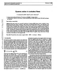
The flow geometry is made of a system of cylindrical columns forming an annulus, as shown in Fig. 1. The

20, 016601-1

© 2008 American Institute of Physics

Author complimentary copy. Redistribution subject to AIP license or copyright, see http://phf.aip.org/phf/copyright.jsp

016601-2

Phys. Fluids 20, 016601 共2008兲

Volk, Odier, and Pinton

columns are grouped in pairs of cyclonic and anticyclonic roll, for which the axial flow is reversed. The velocity is assumed to be stationary and is expressed as the sum of a contribution due to the circular motion of the fluid in a column 关the rotational component VR共r兲兴 and of a contribution due to an axial motion, which we label VA共r兲. In an Earthlike geometry, VA共r兲 would be generated by the Ekman pumping at the upper and lower boundaries. One thus writes

VR

冦

冋

册

VzR共r, ␪兲 = 0,

再 冋

册 冋

V

冦

VrA共z, ␪兲 = 0

冉 冊 冉 冊

␲r ␲z sin共n␪兲sin 2nH 2H ␲ z VzA共z, ␪兲 = cos共n␪兲cos . 2H V␪A共z, ␪兲 =

冧

共3兲

In the second case 关sketched in Fig. 1共b兲兴, the axial flow is reversed about the plane z = 0, hence having symmetries similar to Busse’s columns in rotating convection. Figure 1共e兲 shows a cut of the flow in the plane ␪ = 0. The helicity is therefore negative in the columns of the upper half of the cylinder and positive in the lower half. The axial velocity is then written

VA

冦

VrA共z, ␪兲 = 0

冉 冊

␲r ␲z sin共n␪兲cos nH H ␲z VzA共z, ␪兲 = cos共n␪兲sin . H V␪A共z, ␪兲 = −

冉 冊

冧

共4兲

共1兲

We chose analytical expressions of the fields such that the components are separately divergence-free, ⵜ · VR共r兲 = ⵜ · VA共r兲 = 0. The coefficient ␰ measures the intensity of the axial motion compared to the rotational one. The rotational part in columns of height 2H is expressed in cylindrical polar coordinates as

␲ 共r − 共R − d兲兲 d 1 ␲r ␲ ␲ cos 共r − 共R − d兲兲 + sin 共r − 共R − d兲兲 V␪R共r, ␪兲 = cos共n␪兲 n d d d

VrR共r, ␪兲 = sin共n␪兲 · sin

where n is the number of column pairs, R is the outer radius of the annulus, d is the thickness of the region in which the columns are confined 共within radial distances between R − d and R兲. The velocity is set to zero outside the domain R − d 艋 r 艋 R. For the axial flow, we consider two cases. In the first one, the columns have a height 2H and the axial flow has a defined direction within each column and reverses between neighboring columns. It corresponds to the geometry sketched in Fig. 1共a兲. Figures 1共c兲 and 1共d兲 show, respectively, a cut of the flow in the planes z = 0 and ␪ = 0. The helicity 关H = V · 共ⵜ ⫻ V兲兴 has the same sign in each column, negative in this case 共a column with positive axial velocity rotates with negative vorticity兲. The corresponding velocity is given by

A

V共r兲 = VR共r兲 + ␰VA共r兲.

册冎

冧

共2兲

In our study, we call T1 / 2 the configuration obtained with the rotational velocity and the first choice of the axial velocity field, and T1 the configuration obtained with the second choice. We shall look for stationary solutions of the induction equation,

⳵tB = 0 = ⵜ ⫻ 共V ⫻ B兲 + ␩⌬B,

共5兲

where ␩ is the magnetic diffusivity of the fluid. The boundary conditions are such that the medium inside the annulus has the same electrical conductivity as the fluid while the outside medium is insulating. The magnetic permeability is equal to that of vacuum in the whole space. We stress that once the radius R of the cylinder and the aspect ratio H / R = 2 are fixed there are still many independent parameters which may be varied: the number 2n of columns, their aspect ratio d / R, the magnitude of the axial flow compared to the rotational one, etc. We concentrate on the geometry portrayed in Fig. 1: four pairs of columns with relative thickness equal to 0.4 共yielding a square aspect ratio for the columns兲, and ␰ = 1.25 共this sets the ratio of the maxima of axial to rotational velocities to 0.7, close to the values in the existing experimental dynamos15,17,18兲. The only remaining free parameter is the amplitude of the velocity field, which is nondimensionalized in the form of the magnetic Reynolds number Rm = VmaxR / ␩. Vmax is the maximum velocity in the domain of the flow, and we write V = Vmaxv. B. Iterative procedure

We use here the iterative technique introduced in Ref. 19. The reader is referred to it for a detailed presentation, and for an evaluation of its performance compared to standard analysis in magnetohydrodynamics. This type of selfconsistent approach also underlies the method introduced by Stefani et al.20 For low orders in the development, the method has been previously used for analytical studies,21 including flows with a similar geometry as the one used here.22

Author complimentary copy. Redistribution subject to AIP license or copyright, see http://phf.aip.org/phf/copyright.jsp

016601-3

Phys. Fluids 20, 016601 共2008兲

Dynamo action in an annular array of helical vortices

main. In practice, the boundary conditions are more readily expressed in terms of electric currents and potentials. We thus implement the following sequence: 共i兲

The electromotive force 共emf in units of VmaxB0兲 induced by the flow motion is computed from ek+1 = v ⫻ B k. 共ii兲 Electric current being divergence free, the distribution of electric potential is obtained from ⌬␾k+1 = ⵜ · 共v ⫻ Bk兲, with von Neuman boundary conditions 关n · ⵜ␾ = n · 共v ⫻ B兲, with n the outgoing normal of the domain兴. 共iii兲 Induced currents 共nondimensionalized兲 are then computed as from Ohm’s law jk+1 = −ⵜ␾k+1 + ek+1, and used to compute the magnetic field Bk+1 from the Biot and Savart law. All calculations are made with a magnetic Reynolds number equal to unity 共we set R = 1, Vmax = 1 and ␩ = 1兲. Its actual value enters only in the final step, when contributions are collected and the integer series is computed, B共Rm兲 k . This approach requires that the series con= 兺kBk共Rm = 1兲Rm verges, and sets an upper value for the magnetic Reynolds * 兲. We have found that the radius of connumber Rm 共Rm ⬍ Rm * vergence Rm is of the order of 30; for higher magnetic Reynolds number values we have shown in Ref. 19 that Padé approximants23 still give results in remarkable agreement with the solution of the induction equation computed without approximation. FIG. 1. 共Color online兲 Geometry investigated. 共a兲 Sketch of the column arrangement for the T1 / 2 flow. 共b兲 Column arrangement for the T1 flow. 共c兲 Cut of the T1 / 2 flow in the plane z = 0 共shades correspond to the vertical flow, arrows correspond to the flow in the plane z = 0兲. 共d兲 Cut of the T1 / 2 flow in the plane ␪ = 0. 共e兲 Cut of the T1 flow in the plane ␪ = 0.

We consider the response of the flow to an applied magnetic field B0, looking for the induced field B which solves the stationary induction equation ⵜ ⫻ 共V ⫻ B兲 + ␩⌬B = − ⵜ ⫻ 共V ⫻ B0兲.

共6兲

The result is expressed as the integer series

In this section, we study how, at various stages of the iterative development, several magnetic modes can be obtained as the flow acts on externally applied fields with simple geometries. We will show in the next section how positive feedback loops can be constructed between combinations of the axisymmetric part of these modes. For this reason, as well as for the sake of simplicity, in the present section, the presentation of the induced fields and current densities is restricted to their axisymmetric part. This part is extracted by averaging any given quantity A共r , ␪ , z兲 over the azimuthal angle ␪, 具A典共r,z兲 ⬅

⬁

B = 兺 Bk

III. INDUCTION PROCESSES

with

兩Bk兩 ⬃

k O共Rm 兲B0 .

共7兲

1 2␲

冕

2␲

d␪A共r, ␪,z兲.

共9兲

0

k=1

The contributions Bk are computed iteratively from a hierarchy of nondimensional Poisson equations ⌬Bk+1 = − Rm ⵜ ⫻ 共v ⫻ Bk兲,

k 艌 0,

共8兲

which can be solved for any given set of boundary conditions. C. Numerical simulation

Applying a standard Poisson solver to Eq. 共8兲 would require us to write the complete set of conditions for the magnetic field at the boundaries of the computational do-

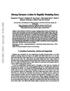
A. Induction from a toroidal applied field

When an external magnetic field is applied in the azimuthal direction 共B0 = B0e␪兲, one expects the generation of an azimuthal current, in very much the same manner as the ␣-effect24 operates in the Roberts flow14 and in the Karlsruhe dynamo.15,25 This is because there is no conceptual difference between a horizontal field transverse to the columns in the Karlsruhe geometry and a toroidal field applied in the geometry considered here. In the azimuthal direction, there is a scale separation between the size of one column and the circumference of the annulus, so the results of mean-field MHD, as for instance explored in Ref. 26 should apply. Note

Author complimentary copy. Redistribution subject to AIP license or copyright, see http://phf.aip.org/phf/copyright.jsp

Phys. Fluids 20, 016601 共2008兲

Volk, Odier, and Pinton

1

1

0.5

0.5

0.5

0.5

0.5

0

0

0

0

0

−0.5

−0.5

−1

0.5 R

1

−0.5

−1

0.5 R

1

Z

1

Z

1

Z

1

Z

Z

016601-4

−0.5

−1

0.5 R

−0.5

−1

1

0.5 R

1

−1

0.5 R

1

FIG. 2. T1 / 2: Applied toroidal field B0,␪. Structure of the azimuthal average 具Bn典 of the fields induced at orders n = 2 , 4 , 6 , 8 , 10.

that in the sequel, although our geometry is not spherical, we shall use the standard term “poloidal” to describe a magnetic field 共or electrical current兲 with field lines in a meridian plane and the term “toroidal” will refer to fields with azimuthal field lines.

effect is indeed present, but the net current J2 is related to the applied field by a full second rank tensor, J2 = ␴关␣兴B0. In the tensor 关␣兴 not all components are due to the flow helicity and some components correspond to an expulsion effect. 2. Higher orders

1. Basic mechanisms at first orders

The topology of B0 is chosen to be identical to the one that would be generated by the flow of an electric current in a rod of radius a located along the z-axis

B0 = B0

冦

r e␪ 共r 艋 a = 0.1兲, a a e␪ 共a 艋 r兲. r

冧

共10兲

The first order having a nonvanishing axisymmetric contribution is the second order. It is illustrated in the left panel of Fig. 2. The poloidal component 共arrows兲 shows a dipolar structure, corresponding to an induced current parallel to the applied field B0 and having the symmetry of the flow helicity; as we have verified, this current is reversed as either vA or vR is reversed but not when both change sign. This type of effect, due to the helical motion in the columns, was first proposed by Parker,27 and evidenced in the VKS experiment.28 It is also in agreement with the ␣-effect introduced in the framework of mean-field magnetohydrodynamics,24 for the 2D array of columns in the Roberts flow,14 and for the columnar ring discussed here.26 Following this analogy, we will call it ␣-effect in the rest of our study. One can also observe on the left panel of Fig. 2 an induced toroidal field 共gray scale兲, largest in the center of the columns and with its direction opposed to the applied field. This remains true even when the rotation of the columns is reversed, or when the axial flow is reversed or even suppressed. The effect traces back to the expulsion of magnetic field lines by vortical motions, as shown by numerical29 and experimental30 studies on an isolated vortex. The response of the flow to an applied field is thus more complex than the generation of an azimuthal current J2,␪ by an ␣-effect due to the helical motion in the columns; this

As detailed in Ref. 19, the interest of the iterative procedure is to associate induction effects with specific actions of velocity gradients. It is particularly convenient when a patterns develops through the iterations. As it is the case here, we define a tool to help us quantify the convergence of the pattern. Let B j and Bk be the fields induced at respective orders j and k. We compute the scalar product 共B j兩Bk兲 =

1 2 ␲ R 2H

冕

d3rB j · Bk ,

共11兲

V

and the associated norm N共Bk兲 = 冑共Bk 兩 Bk兲. Comparisons are made using the normalized scalar product P j,k =

冉

Bj

兩

Bk

N共B j兲 N共Bk兲

冊

.

共12兲

In the case of an azimuthal applied field, the expulsion eventually dominates. To wit, we compare in Fig. 2 successive iterations of the magnetic field 具B2k典. One finds P2,4 ⬃ −0.95, while P2,3 ⬍ 10−3; the field induced at fourth order is almost exactly opposed to B2 and perpendicular to B3. As a result, the successive induction steps lead to the expulsion of the applied field, with Pk,k+1 ⬃ 0 and Pk,k+2 ⬃ −1, at higher orders. Bear in mind that this concerns normalized values. In dimensional units, one has Bk+2 ⬃ ␥Bk,

with ␥ ⬃ − 1/400.

共13兲

After the tenth order, we could not detect any appreciable evolution of the pattern. 3. Evolution with Rm

The magnetic Reynolds number is reintroduced in the ⬁ k summation Bind = 兺k=1 Rm Bk. We have summed terms up to order 22, resulting in a 1% accuracy. We show in Fig. 3 the evolution with Rm of two components of the induction: the

Author complimentary copy. Redistribution subject to AIP license or copyright, see http://phf.aip.org/phf/copyright.jsp

016601-5

Phys. Fluids 20, 016601 共2008兲

Dynamo action in an annular array of helical vortices

pade order 22 order 2

1

0.8

1

0.8

0.6

1

0.6

0.4

*

0.2

0 0

0.4

10

20

*

0.2

30

40

0 0

50

10

20

(a)

30

40

50

(b)

FIG. 3. 共Color online兲 T1 / 2: evolution with Rm. 共a兲 Axial field in the center of the annulus, at 共r = 0, z = 0兲; 共b兲 toroidal field in the columns, at 共r = 0.8, z = 0兲. Rm* is the radius of convergence of the integer series. The dashed line corresponds to the summation stopped at order 2, the continuous line with dots to the summation up to order 22, and the continuous line to the summation using Padé approximants.

axial field in the center of the cylinder, and the toroidal field in the center of the columns. For Rm 艋 8, the calculation at second order yields a very good approximation of the net induction. This is interesting because the second order truncation corresponds to the computation of the mean-field theory with a first order smoothing approximation.26 For magnetic Reynolds numbers greater than about 8, the contributions of higher orders in the summation need to be taken into account. One finds that the mean-field approximation tends to overestimate the induced dipole field, Fig. 3共a兲, as well as the expulsion of the toroidal field, Fig. 3共b兲. Empirically, we observe that the radius of convergence * = 17. This value can be understood of the integer series is Rm from our observation that Pk,k+1 ⬃ 0 and Bk+2 ⬃ ␥Bk. Indeed one can then rewrite the summation as 共14兲

k=0

from which one immediately gets 1 / 冑兩␥兩 ⬃ 20 for the radius * , one gets of convergence. In addition, for Rm ⬍ Rm B⯝

2 Rm

Rm 2 B1 + 2 B2 , 1 + 兩␥兩Rm 1 + 兩␥兩Rm

B0 = B0

共15兲

which shows that the divergence of the integer series actually lies in the existence of imaginary roots. Such a configuration is particularly suited to the use of Padé approximants.23 The result, plotted as a solid line in Fig. 3, shows that at large magnetic Reynolds numbers 共Rm 艌 40兲 the axial induction and the expulsion may saturate. B. Induction from a radial field applied

As detailed above, starting from an applied toroidal field, the ␣-effect generates a poloidal induced field with a large axial component. But this axial component gives in turn very weak contributions to the induction; an applied field in the axial direction induces fields that are two orders of magnitude weaker than the values obtained with other orientations.

冦

r er 共r 艋 a = 0.1兲 a a er 共a 艋 r兲. r

冧

共16兲

Two remarks about this functional form are in order: 共i兲

共ii兲

⬁

2 2 k B2兲 兺 共− 兩␥兩Rm 兲 , B = 共RmB1 + Rm

In contrast, we show in this section that a radially applied field generates an induced field which has a significant component in the azimuthal direction. Specifically, we consider an applied field B0 of the form

Within the domain of resolution of the induction equation it is essential that B0 be divergence free because we solve iteratively ⌬Bk+1 = −ⵜ ⫻ 共v ⫻ Bk兲 rather than ⌬Bk+1 = −v · ⵜBk − Bk · ⵜv. Here, B0 is not divergence free for r 艋 a, but in this domain the source term in ⌬B1 = −ⵜ ⫻ 共v ⫻ B0兲 vanishes with v.

1. Basic mechanisms

For one individual column, a radial applied field is very similar to a toroidal applied field. Therefore, one expects the same mechanisms to be at play. The screw motion in the columns produces again a current parallel to the applied field. The current lines close inside the conducting fluid, leading to two poloidal loops. They generate a field 具B2典 whose toroidal part is antisymmetric about the z = 0 plane, as shown in Fig. 4 共left panel兲. The arrows in the same figure correspond to a poloidal field whose radial component is opposed to the applied field, as expected from an expulsion mechanism at play in the center of each column. In terms of amplitude, the radial/azimuthal conversion generated by the ␣-effect is of the same order of magnitude as the reverse process, discussed in the previous section. One computes max兵具B2,␪典 / B0,r其 ⬃ 7 · 10−4, to be compared to max兵具B2,r典 / B0,␪其 ⬃ 11· 10−4 obtained in the case of the azimuthal applied field. However, the major difference is that

Author complimentary copy. Redistribution subject to AIP license or copyright, see http://phf.aip.org/phf/copyright.jsp

016601-6

Phys. Fluids 20, 016601 共2008兲

Volk, Odier, and Pinton

0.5

0.5

0.5

0.5

0.5

0

0

0

0

0

−0.5

−1

−0.5

0.5 R

−0.5

−1

1

0.5 R

−0.5

−1

1

Z

1

Z

1

Z

1

Z

1

Z

1

0.5 R

1

−0.5

−1

0.5 R

−1

1

0.5 R

1

FIG. 4. T1 / 2: applied radial field B0,r. Structure of the azimuthal average 具Bn典 of the fields induced at orders n = 2 , 4 , 6 , 8 , 10.

the expulsion is much weaker. The component of 具B2典 opposed to the applied radial field is 10 times weaker than the induced toroidal field. This can be explained by the fact that, while B2 has a component opposed to the applied field in the center of the columns, it has a contribution which reinforces the applied field in their periphery. Therefore, when the azimuthal average is computed, the expulsion effect is weakened. On the contrary, in the case of the azimuthal applied field, the expulsion effects from each column was adding up collectively, resulting in a larger contribution. Hence, expulsion is less effective in the direction perpendicular to the direction where scale separation develops 共in the azimuthal direction the columns cross section is an order of magnitude smaller than the cylinder diameter, while in the radial direction the characteristic size of the flow is equal to the width of the column兲. We conclude that in the case considered here, scale separation does not particularly favor magnetic induction, but dramatically reduces expulsion.

2. Higher orders

The structure of the induced magnetic field is rapidly stabilized towards a quadrupolar structure as higher orders are computed. As shown in Fig. 4 the fields at all even orders closely resemble that at order 2, with a change of sign between consecutive even orders; the normalized scalar products are P2,4 ⬃ −0.70 and P4,6 ⬃ −0.92. The fields produced at a given order are again fairly orthogonal to the fields at next or previous order: 共Bk 兩 Bk+1兲 ⬃ 0. In addition, as can be seen in Fig. 4, the iteration converges for even orders towards a quadrupolar structure with a negative feedback in a two step mechanism, Bk+2 = − ␥Bk 共␥ ⬃ 1/415兲.

共17兲

3. Evolution with Rm

The Rm dependence of the induced radial and azimuthal magnetic field is shown in Fig. 5, after summation of the

1 1.6

pade order 22 order 2

1.5 1.4

0.9 0.8 0.7 0.6

1.2

0.5

1.1

0.4

1

0.3

1

r

1.3

0.9

0.7 0

0.2

*

0.8 5

10

15

*

0.1 20

(a)

25

30

35

40

45

0 0

5

10

15

20

25

30

35

40

45

(b)

FIG. 5. 共Color online兲 T1 / 2: induction at higher orders for an applied radial field B0,r. Variation with Rm of the induced fields. 共a兲 Radial induced component, sampled at 共r = 0.7, z = 0兲. 共b兲 Azimuthal induced component, sampled at 共r = 0.7, z = −0.6兲. The dashed line corresponds to the summation stopped at order 2, the continuous line with dots to the summation up to order 22, and the continuous line to the summation using Padé approximants.

Author complimentary copy. Redistribution subject to AIP license or copyright, see http://phf.aip.org/phf/copyright.jsp

016601-7

Phys. Fluids 20, 016601 共2008兲

Dynamo action in an annular array of helical vortices

terms up to order 22. Note that B␪ is sampled at 共r = 0.7, z = −0.6兲, because for a quadrupole, the toroidal field is very weak in the z = 0 plane. One observes in Fig. 5共b兲 that a second order calculation is a correct approximation for magnetic Reynolds numbers up to 10. For higher Rm other terms need to be included. As in the case of the toroidal applied field, they tend to slow the increase of the induced field, mainly because of expulsion generated from rotational mo* = 18, tion in the columns. The integer series diverges for Rm as expected from the value 1 / 冑兩␥兩 ⬃ 20. Results obtained using Padé approximants, although extending the computed induction beyond the radius of convergence of the series, do not point to a saturation at large Rm. IV. DYNAMO ACTION

In the previous section, we showed that the induction mechanisms in the case of the T1 / 2 flow consist of a mutual conversion between azimuthal and radial fields, through the ␣-effect, along with an effect of expulsion of these fields by the rotating columns. We have identified two modes, dipole and quadrupole, mainly axisymmetric, that realize a feedback loop in a two-step mechanism 关Eqs. 共13兲 and 共17兲兴 with a negative sign, therefore leading to an antidynamo configuration. Following the ideas developed in Ref. 19, we can express these results using an induction operator formalism. From Eq. 共8兲, we define L共Rm兲 ⬅ −Rm⌬−1兵ⵜ ⫻ 共v ⫻ · 兲其 for a velocity field v corresponding to the value Rm = 1. Equations 共13兲 and 共17兲 can then be interpreted in the following way: the 具B2n典 modes 共n ⬎ 5兲 obtained in the induction studies in Secs. III A 共dipole mode兲 and III B 共quadrupole mode兲 are eigenvectors of L2共Rm兲. From this observation, we will show in this section that using a poloidal/toroidal decomposition, a matrix analysis can be performed on the identified eigenmodes to find eigenvectors of L2共Rm兲 with positive eigenvalues, thus leading to possible dynamo solutions. Writing for simplicity L = L共1兲 关we then have L共Rm兲B = RmLB兴, let us assume that we can find a magnetic field Be that is not an eigenvector of the operator L, but of L2 with a positive eigenvalue ␥e; then, Bs = Be + 1 / 冑␥eLBe is an eigenvector of L with a positive eigenvalue ␥s = 冑␥e. Taking Rm = 1 / 冑␥e, we then have L共Rm兲Bs = Bs, which defines Bs as a self-sustained magnetic field in the corresponding velocity field, at threshold Rm = 1 / 冑␥e. We emphasize that this method is more complex than an eigenvalue calculation. In addition, as will become clearer later, it does not strictly respect the symmetries,16 since approximations have to be made when projecting the results of the application of the operator L2 onto the initial vectors. We will discuss the validity of all approximations and show that the technique helps understanding not only the dynamo modes and their thresholds but also how the induction effects can combine to produce a dynamo. A. Dynamo action in the T1 / 2 flow

We first illustrate our method with an example: the generation of a dipole field for a given flow. We use this example to estimate the error associated to the approximations made in the method.

1. Method and error estimates: Example of the generation of a dipole field

We start from the field 具B10典 共Fig. 2兲, which was shown 关Eq. 共13兲兴 to be an eigenvector of L2, with a dipolar geometry and a negative eigenvalue. Since a dynamo cycle is often seen as a toroidal/poloidal feedback loop,12 we decompose this field into its toroidal—BTd —and poloidal— BdP—components, to which we apply the operator L2. As expected, the resulting fields are of opposite sign with respect to BTd and BdP. In addition, their topology are very similar and look like a linear combination of the initial fields BTd and BdP. Using the scalar products defined in Eq. 共11兲, we can project 具L2BTd 典 and 具L2BdP典 onto the initial fields, thus defining an induction matrix, M d共T1/2兲 = =

冉

冉

M PP M PT M TP M TT

冊

共具L2BdP典兩BdP兲 共具L2BdP典兩BTd 兲 共具L2BTd 典兩BdP兲 共具L2BTd 典兩BTd 兲

冊

,

共18兲

where we have taken N共BTd 兲 = N共BdP兲 = 1, using the norm N defined in Sec. III A 2. This matrix M d共T1 / 2兲 is the restriction of the two-step induction operator L2 to the vector space of the axisymmetric dipoles. The diagonal terms represent the expulsion effect and the extra-diagonal terms represent the action of the ␣-effect. Positive eigenvalues correspond to an axisymmetric dipolar dynamo. Let us discuss the approximations made in this method. We have assumed so far that 具L2BTd 典 and 具L2BdP典 belong to the vector space generated by BTd and BdP. In order to check the validity of this hypothesis, we show some comparisons in Fig. 6, using profiles normalized by their maximum value: in 共a兲 the axial profiles of the radial component of 具L2BTd 典 and 具L2BdP典 are compared to the equivalent profile for BdP. One can see that the overlap is very good. In 共b兲, the radial profiles of the azimuthal component of 具L2BTd 典 and 具L2BdP典 are compared to the radial profile for BTd . In the case of the ␣-effect 共具L2BdP典 profile兲, the overlap is very good again. In the case of the expulsion effect 共具L2BTd 典 profile兲, there is a discrepancy. We have computed the error to be about 10%. Thus the M TT term in the matrix represents the expulsion mechanism for the applied toroidal field within an error of 10%, while the other elements of the matrix can be considered as correct within less than 1%.

2. General expression for the matrix M

By redefining the L operator as a linear function of the poloidal and toroidal components of the flow, we obtain a general expression of the matrix M, for any value of the axial/rotational ratio 共␰ parameter兲. We normalize the components vA and vR of the velocity field, max共vA兲 = 1 and max共vR兲 = 1 and rewrite Eq. 共1兲 as V = VAvA + VRvR, where VA and VR represent the maximum amplitude of each component. Let LA be the induction operator when V = vA and LR be the induction operator when V = vR; L can then be written as the linear combination,

Author complimentary copy. Redistribution subject to AIP license or copyright, see http://phf.aip.org/phf/copyright.jsp

016601-8

Phys. Fluids 20, 016601 共2008兲

Volk, Odier, and Pinton 1

1.2

0.8

1

0.6

0.8

0.4

0.6

θ

Br

0.2

B

0

-0.2 -0.4

0.4 0.2

-0.6

0

-0.8 -1 -1

0

-0.5

0.5

1

-0.2

0

0.2

0.4

Z (a)

0.6

0.8

1

r (b)

FIG. 6. 共Color online兲 Dipolar mode: estimate of the error made doing the projection 共a兲 axial profile of Br at r = 0.8 from the Oz axis. 共b兲 Radial profile of B␪ in the median plane. 共䊏兲: Components of the applied field. 共⽧兲: Components of 具L2BdP典. 共쎲兲: Components of 具L2BTd 典.

L = V AL A + V RL R ,

共19兲

M q共VA,VR兲 = − 10−4

yielding L2 = VA2 LALA + VAVR共LRLA + LALR兲 + VR2 LRLR ,

共20兲

so that the four matrix elements M ij can also be written as quadratic forms of VA and VR, 共21兲

M ij = aijVA2 + bijVRVA + cijVR2 .

As we studied the induction mechanisms, we noticed that the ␣-effect and the expulsion behave differently under a reversal of the axial pumping 共VA → −VA兲 or of the columns rotation 共VR → −VR兲. More precisely, it was observed that the expulsion effect is independent of these sign changes, whereas the ␣-effect transforms as the product VAVR. These observations allow to eliminate some terms in Eq. 共21兲, yielding M共VR,VA兲 =

冉

aVR2 + bVA2

cVRVA

dVRVA

eVR2 + fVA2

冊

共22兲

.

We will now compute the value of these six coefficients in the case of the T1 / 2 flow. The corresponding expressions for the matrix M are the following: Axial dipole: We use here the axial dipole basis, defined in Sec. IV A 1, M d共VA,VR兲 = − 10

−4

冉

22VA2 + 6VR2

46VAVR

18VAVR

14共VA2 + VR2 兲

冊

冉

23VA2 + 5VR2

25VAVR

25VAVR

11共VA2 + VR2 兲

冊

.

共24兲

Transverse dipole: Until now, we have only considered axisymmetric fields. However, since the T1 / 2 flow presents several analogies with the Roberts flow, it would be interesting to study the possibility of generating a transverse dipole 共perpendicular to the columns兲, as observed in the Karlsruhe dynamo.15 We follow the same strategy as before: a uniform transverse field B0 = B0ex 共where the direction of ex is given by ␪ = 0, see Fig. 1兲 is applied to the flow and we compute the fields Bk obtained after k iterations. They rapidly converge towards a stable structure. After 8 iterations, the fields Bk and L2Bk have an overlap close to 100%, and the eigenvalue is negative, ␥ = −1 / 400. This nonaxisymmetric mode cannot be decomposed into a poloidal and toroidal part but we noticed previously that this decomposition also separated symmetric and antisymmetric components, under the reflection symmetry with respect to the plane z = 0. In the same way, the mode B8 obtained here can be decomposed into its symmetric and antisymmetric parts, that form a generating basis. Using this basis, the matrix M is M t共VA,VR兲 = − 10−4

冉

22VA2 + 13VR2

29VAVR

46VAVR

16VA2 + 14VR2

冊

. 共25兲

3. Dynamo capability of T1 / 2 flow

.

共23兲

Axial quadrupole: In this case, the generating vectors are formed by the poloidal and toroidal components of the field 具B10典 presented in Fig. 4, which was shown 关Eq. 共17兲兴 to be an eigenvector of the operator L2, with a quadrupolar geometry and a negative eigenvalue. This mode is orthogonal to the dipole mode,

From the expressions of the matrix M obtained in the previous paragraph, the largest eigenvalue ␭max of each matrix can be computed as a function of VA and VR. The result is shown in Fig. 7. In order to facilitate the reading of these plots, when ␭max was negative 共no dynamo兲, we artificially set its value to zero. For each case, two regions are evidenced: the first one, for which ␭max ⬎ 0, corresponds to the possibility to observe a dynamo for the considered

Author complimentary copy. Redistribution subject to AIP license or copyright, see http://phf.aip.org/phf/copyright.jsp

016601-9

Phys. Fluids 20, 016601 共2008兲

Dynamo action in an annular array of helical vortices

10

-4

2

1 Axial dipole

10

2

1.5

VA 0.5

-4

1 Quadrupole

V A 0.5

1

1 0.5

0

1

0

0

0.5

0

1

1

0.5

0

VR

VR

(a)

(b)

10

-4

4

Transverse dipole

1 No dynamo

Transverse

3

VA0.5

2

Dipole

VA 0.5

ed

in

0

0.5

1

0

un

m er

Quadrupole

et

d

1

0

0

No dynamo 0

0

0.5

VR

VR

(c)

(d)

1

FIG. 7. 共Color online兲 T1 / 2 flow: evolution of the largest eigenvalue of the induction matrix in the 共VR , VA兲 plane. 共a兲 Axial dipole; 共b兲 axial quadrupole; 共c兲 transverse dipole; 共d兲 predominance diagram for the different possible modes. For simplicity, when the eigenvalue is negative we plotted a zero value.

geometric parameters 共d / r = 0.4 and n = 4兲 with a threshold c = 1 / 冑␭max. The second, for which ␭max ⬍ 0, corresponds Rm to the case where no dynamo instability can take place. Figures 7共a兲–7共c兲 show that the three dynamo modes coexist in the same region, in the neighborhood of the line VA = VR. This is not surprising, since when one of the velocity component dominates the other, the expulsion mechanism is more important than the ␣-effect, which needs both components together. For a given couple 共VA , VR兲, one can observe that ␭q is always larger than ␭d 共corresponding to a lower threshold兲. In the same way, the transverse dipole always has a lower threshold than the axial dipole. A summary of the predominance of the different modes is given in Fig. 7共d兲, where one can see that the transverse dipole is favored by higher ratio axial/rotational, whereas the quadrupole is favored by a lower ratio. The case of the transverse dipole mode is interesting, since it sheds light on the Karlsruhe dynamo, using the

analogies between the T1 / 2 flow and the Roberts flow. As suggested earlier in Refs. 31 and 32, along the two directions perpendicular to the pipes, the two components of the field transform into one another through an ␣-effect. In a T1 / 2 flow, we thus observed that several dynamo modes can be sustained when Rm ⯝ 80. This result is consistent with other numerical studies in thermal convection,33 which have shown that various dynamo solutions can coexist in the same region of the parameter space. This kind of behavior has also been observed in the VKS dynamo experiment,34 where different dynamo modes 共steady, chaotically reversing, bursts, periodic兲 can be obtained when changing the rotation rate of the driving impellers. B. Dynamo mechanisms in the T1 flow

The analytical expression of the T1 flow is given in Eq. 共4兲. Compared to the T1 / 2 flow 关Eq. 共3兲兴, the only difference is that the azimuthal and axial components are now, respec-

Author complimentary copy. Redistribution subject to AIP license or copyright, see http://phf.aip.org/phf/copyright.jsp

016601-10

Phys. Fluids 20, 016601 共2008兲

Volk, Odier, and Pinton P

B2

10

T

B0

(a)

T

J2

7.5 B

(b)

T

symmetric mode

B0

P 2

VA

T

J2

5

2.5

P

B2

(c)

T

antisymmetric mode

B0

0

T

J2

FIG. 8. 共Color online兲 Comparison between the schematic induction mechanisms for the T1 / 2 and T1 flows, due to the ␣-effect in the case of a toroidal applied field. The lines in the second column represents the applied field, and in the third column, the dashed line represents the resulting order 2 current and the solid line the resulting order 2 magnetic field. 共a兲 T1 / 2 flow; 共b兲 T1 flow, with a symmetric applied field; 共c兲 T1 flow, with an antisymmetric applied field.

tively, symmetric and antisymmetric under Sz. T1 is a superposition of two T1 / 2 flows, one in each half-cylinder, symmetric with respect to Sz. They have opposite helicity, since their axial component is reversed, while the rotation of the columns is unchanged. The strong similarity between the T1 / 2 and T1 flows indicates that the same mechanisms, ␣-effect and expulsion, will take place. Figure 8 compares the schematic induction mechanisms for the ␣-effect in both types of flow. In 共a兲, the case of the T1 / 2 flow is recalled, where the induced current 共j = ␴␣B兲 is parallel to the applied field with the same sign, since helicity H is negative in this flow and the ␣ coefficient is proportional to −H. In 共b兲, it is shown that in the T1 flow, applying a symmetric toroidal field results in a symmetric poloidal field, corresponding to a quadrupolar geometry. In 共c兲, we show that the dipolar geometry 共antisymmetric poloidal field兲 is obtained by applying an antisymmetric toroidal field. Based on these symmetry considerations, the dipolar mode for the T1 flow was built by applying L iteratively to an initial toroidal field antisymmetric with respect to Sz. We chose an initial field of the form B0 = B0 sin共␲z / H兲e␪. The iterations converge rapidly towards a mode whose toroidal and poloidal parts, once the azimuthal average is done, form a basis which is closed under the action of L2. In the same way, the quadrupolar generating basis was constructed starting from an azimuthal z-independent field 关note that an identical mode is obtained if one starts from a symmetric radial field of the form B0 = B0a / r cos共␲z / H兲er兴. As for the transverse mode, we tried to follow the same procedure used in the case of the T1 / 2 flow, but it turned out that the converged mode, starting from an initial uniform transverse field, is formed of two dipolar structures at 90° from each other, having the same behavior under the reflection symmetry with respect to the plane z = 0. Therefore, it is

VR FIG. 9. 共Color online兲 T1 flow: evolution of the largest eigenvalue of the induction matrix in the 共VR , VA兲 plane, for the axial quadrupole. For simplicity, when the eigenvalue is negative we plotted a zero value.

not possible to use this symmetry to construct the basis vectors. And we were indeed unable to find any basis that would be closed under the action of L2. This shows a limitation of our method. The expressions for the matrix M obtained are: Dipolar mode: M d共VA,VR兲 = − 10−4

冉

16VA2 + 8VR2

33VAVR

16VAVR

12共VA2 + VR2 兲

冊

.

共26兲

There is no value of the couple 共VA , VR兲 for which the axial dipole can be sustained by the T1 flow. Some studies have shown35 that in order for a T1-type flow to sustain an axial dipole, the presence of differential rotation, absent in our study, would be necessary. Axial quadrupole: M q共VA,VR兲 = − 10−4

冉

20VA2 + 5VR2

25VAVR

20VAVR

11VA2 + 8VR2

冊

.

共27兲

Figure 9 shows the evolution of ␭max in the case of the quadrupole mode. It is interesting to note that in all the cases where a dynamo was possible, the corresponding matrix 关M d共T1 / 2兲, M q共T1 / 2兲, M t共T1 / 2兲, and M q共T1兲兴 presented the following characteristics: one could find values of the couple 共VA , VR兲 so that the product of the nondiagonal terms was larger than the product of the diagonal terms. One can easily show that this is a necessary and sufficient condition for a 2 ⫻ 2 matrix 共with negative diagonal coefficients兲 to have a positive eigenvalue. And this condition physically corresponds to the facts that the expulsion mechanism 共diagonal terms兲 is weaker than the ␣ mechanism 共nondiagonal terms兲. On the contrary, in the case of 关M d共T1兲兴, this condition is not met. V. CONCLUDING REMARKS

A better understanding of the MHD induction mechanisms in a given system can help to build dynamo cycles. In

Author complimentary copy. Redistribution subject to AIP license or copyright, see http://phf.aip.org/phf/copyright.jsp

016601-11

Phys. Fluids 20, 016601 共2008兲

Dynamo action in an annular array of helical vortices

the first part of this study, we have identified two mechanisms, related, respectively, to the ␣-effect and to expulsion by vortices. We expressed these mechanisms in terms of the induction operator L2 and, using a poloidal/toroidal decomposition of the eigenvectors of L2, we were able to perform a matrix analysis leading to the determination of self-sustained magnetic modes. This analysis not only allows to predict a threshold for these dynamo modes, as could indeed have been computed using more standard eigenvalue computation, but the additional benefit is that it also brings a new insight into these modes, providing the actual induction mechanisms which combine to produce a dynamo effect. In regards to natural or experimental conditions, it helps understand which features of the velocity field favor or hinder dynamo action. In addition, as already noticed in other studies,36 the competition between the ␣-effect, favorable to the dynamo, and the expulsion effect, that works against it, can be monitored by the ratio of poloidal to toroidal components of the velocity field 共in our case the axial to rotational ratio VA / VR兲. Our studies show that a positive feedback requires a comparable amplitude for rotation and pumping. In the case of the T1 / 2 flow 共for eight columns and an aspect ratio of 0.4兲, we observed that both axisymmetric modes 共dipolar and quadrupolar兲 can be sustained, with a threshold of the order of Rm = 100. We also showed that a transverse dipole mode can exist, as one could expect, because of the analogy between our flow and the Karlsruhe dynamo. On the other hand, the T1 flow can only sustain a quadrupolar mode, when the pumping amplitude is larger than the rotation amplitude. For the axial dipole mode, the poloidal to toroidal conversion seems too weak to compensate for the strong expulsion of the azimuthal field. This study also provides a better understanding of the role of scale separation; it does not particularly enhance the induction effects, but rather reduces the field expulsion in the direction perpendicular to the separation, thus indirectly favoring the dynamo process. Coming back to the Earth’s case, our model system leads to several observations. An ␣2 dynamo process relies on the helicity contained in Busse’s columns,5 but Ekman pumping would give a very weak source of axial motion, since the Ekman number E is of the order of 10−15 and the ratio of the axial flow to the rotational flow scales like E1/2.37 Another source of axial velocity could be the ␤-effect due to the curvature of the core-mantle boundary—note that in this case the axial flow is in phase with the radial flow rather than with the vorticity.35 A large scale dipole field could also be generated from an ␣ − ␻ dynamo. It would require differential rotation as provided, for instance, by zonal winds38,39 or super-rotation effects as observed in the DTS laboratory experiment.40 These ingredients could in principle be added to the model studied here, and the procedure used to determine which dynamo modes 共dipole, quadrupole or other兲 are likely to exist for a given range of Reynolds numbers. As proposed for geomagnetism,41 and recently observed in the VKS experiment,34 the close proximity of dynamo modes may be essential for the development of dynamical regimes.

ACKNOWLEDGMENTS

We acknowledge useful discussions with M. Bourgoin, R. Avalos-Zuñiga, P. Cardin, F. Plunian, and N. Schaeffer. This work was partially supported by the Émergence Program of the Rhône-Alpes Region 共France兲. 1

J. Larmor, “How could a rotating body such as the sun become a magnet?” Report of the 87th meeting of the British Association for the Advancement of Science 共1919兲, pp. 159–160. 2 J.-P. Poirier, “Physical properties of the Earth core,” C. R. Seances Acad. Sci. II 318, 341 共1994兲. 3 S. Labrosse, “Thermal and magnetic evolution of the Earth core,” Phys. Earth Planet. Inter. 140, 127 共2003兲. 4 S. L. Butler, W. R. Peltier, and S. O. Costin, “Numerical models of the Earth’s thermal history: Effects of inner-core solidification and core potassium,” Phys. Earth Planet. Inter. 152, 22 共2005兲. 5 F. H. Busse, “Thermal instabilities in rapidly rotating systems,” J. Fluid Mech. 44, 441 共1970兲; C. R. Carrigan and F. H. Busse, “An experimental investigation of the onset of convection in rotating spherical shells,” ibid. 126, 287 共1983兲. 6 U. R. Christensen, J. Aubert, P. Cardin, E. Dormy, S. Gibbons, G. A. Glatzmaier, E. Grote, Y. Honkura, C. Jones, M. Kono, M. Matsushima, A. Sakuraba, F. Takahashi, A. Tilgner, J. Wicht, and K. Zhang, “A numerical dynamo benchmark,” Phys. Earth Planet. Inter. 128, 25 共2001兲; E. Dormy, A. M. Soward, C. A. Jones, D. Jault, and P. Cardin, “The onset of thermal convection in rotating spherical shells,” J. Fluid Mech. 501, 43 共2004兲. 7 E. Dormy, J.-P. Valet, and V. Courtillot, “Numerical models of the geodynamo and observational constraints,” Geochem., Geophys., Geosyst. 1, 62 共2000兲. 8 V. Morin and E. Dormy, “Dissipation mechanisms for convection in rapidly rotating spheres and the formation of banded structures,” Phys. Fluids 18, 068104 共2006兲. 9 H. Harder and U. Hansen, “A finite volume solution method for the thermal convection and dynamo problem is spherical shells,” Geophys. J. Int. 161, 522, DOI: 10.1111/j.1365-246X.2005.02560.x 共2005兲. 10 V. Morin, Ph.D. thesis, Université Denis Diderot-Paris 共2005兲. 11 F. H. Busse, “Convective flows in rapidly rotating spheres and their dynamo action,” Phys. Fluids 14, 1301 共2002兲. 12 H. K. Moffatt, Magnetic Field Generation in Electrically Conducting Fluids 共Cambridge University Press, Cambridge, 1978兲. 13 E. Grote, F. H. Busse, and A. Tilgner, “Convection-driven quadrupolar dynamos in rotating spherical shells,” Phys. Rev. E 60, R5025 共1999兲. 14 G. O. Roberts, “Dynamo action of fluid motions with two-dimensional periodicity,” Philos. Trans. R. Soc. London, Ser. A 271, 41 共1972兲. 15 R. Stieglitz and U. Müller, “Experimental demonstration of a homogeneous two-scale dynamo,” Phys. Fluids 13, 561 共2001兲. 16 A. Tilgner, “Small scale kinematic dynamos: beyond the ␣-effect,” Geophys. Astrophys. Fluid Dyn. 98, 225, DOI: 10.1080/ 0309192042000196103 共2004兲. 17 A. Gailitis, O. Lielausis, S. Dement’ev, E. Platacis, and A. Cifersons, “Detection of a flow induced magnetic field eigenmode in the Riga dynamo facility,” Phys. Rev. Lett. 84, 4365 共2000兲. 18 R. Monchaux, M. Berhanu, M. Bourgoin, M. Moulin, Ph. Odier, J.-F. Pinton, R. Volk, S. Fauve, N. Mordant, F. Pétrélis, A. Chiffaudel, F. Daviaud, B. Dubrulle, C. Gasquet, L. Marié, and F. Ravelet, “Generation of magnetic field by dynamo action in a turbulent flow of liquid sodium,” Phys. Rev. Lett. 98, 044502 共2007兲. 19 M. Bourgoin, P. Odier, J.-F. Pinton, and Y. Ricard, “An iterative study of time independent induction effects in magnetohydrodynamics,” Phys. Fluids 16, 2529 共2004兲. 20 See also F. Stefani, G. Gerbeth, and K. H. Rädler, “Steady dynamos in finite domains: An integral equation approach,” Astron. Nachr. 321, 65 共2000兲. 21 K.-H. Rädler, M. Rheinhardt, E. Apstein, and H. Fuchs, “On the meanfield theory of the Karlsruhe dynamo experiment,” Nonlinear Processes Geophys. 9, 171 共2002兲. 22 F. H. Busse, “A model of the geodynamo,” Geophys. J. 42, 437 共1975兲. 23 W. H. Press, S. A. Teukolsky, W. T. Vetterling, and B. P. Flannery, Numerical Recipes 共Cambridge University Press, Cambridge, 1986兲.

Author complimentary copy. Redistribution subject to AIP license or copyright, see http://phf.aip.org/phf/copyright.jsp

016601-12 24

Volk, Odier, and Pinton

F. Krause and K.-H. Rädler, Mean Field Magnetohydrodynamics and Dynamo Theory 共Pergamon, New York, 1980兲. 25 A. Tilgner, “A kinematic dynamo with a small scale velocity field,” Phys. Lett. A 226, 75 共1997兲. 26 R. A. Avalos-Zuñiga, F. Plunian, and K. H. Rädler, “Mean electromotive force generated by a ring of helical vortices,” in Proceedings of the 21st ICTAM, 15–21 August 2004, Warsaw, Poland, edited by W. Gutkowski and T. A. Kowaleski 共Springer, Dordrecht, The Netherlands, 2005兲. 27 E. N. Parker, “Hydromagnetic dynamo models,” Astrophys. J. 122, 293 共1955兲. 28 F. Pétrélis, M. Bourgoin, L. Marié, J. Burguete, A. Chiffaudel, F. Daviaud, S. Fauve, P. Odier, and J.-F. Pinton, “Non linear magnetic induction by helical motion in a liquid sodium turbulent flow,” Phys. Rev. Lett. 90, 174501 共2003兲. 29 N. O. Weiss, “The expulsion of magnetic flux by eddies,” Proc. R. Soc. London, Ser. A 293, 310 共1966兲. 30 P. Odier, J.-F. Pinton, and S. Fauve, “Magnetic induction by coherent vortex motion,” Eur. Phys. J. B 16, 373 共2000兲. 31 F. H. Busse, “Magnetohydrodynamics of the Earth’s Dynamo,” Annu. Rev. Fluid Mech. 10, 435 共1978兲. 32 P. H. Roberts and A. M. Soward, “Dynamo theory,” Annu. Rev. Fluid Mech. 24, 459 共1992兲. 33 J. Aubert and J. Wicht, “Axial vs. equatorial dipolar dynamos models with

Phys. Fluids 20, 016601 共2008兲 implications for planetary magnetic fields,” Earth Planet. Sci. Lett. 221, 409 共2004兲. 34 M. Berhanu, R. Monchaux, S. Fauve, N. Mordant, F. Pétrélis, A. Chiffaudel, F. Daviaud, B. Dubrulle, L. Marié, F. Ravelet, M. Bourgoin, Ph. Odier, J.-F. Pinton, and R. Volk, “Magnetic field reversals in an experimental turbulent dynamo,” Europhys. Lett. 77, 59001 共2007兲. 35 N. Schaeffer and P. Cardin, “Quasi-geostrophic kinematic dynamos at low magnetic Prandtl number,” Earth Planet. Sci. Lett. 245, 595 共2006兲. 36 M. Bourgoin, R. Volk, P. Frick, S. Kripechenko, P. Odier, and J.-F. Pinton, “Induction mechanisms in von Kármán swirling flows of liquid gallium,” Magnetohydrodynamics 40, 3 共2004兲. 37 H.-C. Nataf and J. Sommeria, La physique et la Terre 共Éditions Belin, CNRS éditions, Paris, 2000兲. 38 N. Gilet, Ph.D. thesis, Université Joseph Fourier, Grenoble 1 共2004兲. 39 J. Aubert, Ph.D. thesis, Université Joseph-Fourier, Grenoble 1 共2001兲. 40 H-C. Nataf, T. Alboussire, D. Brito, P. Cardin, N. Gagnire, D. Jault, J-P. Masson, and D. Schmitt, “Experimental study of super-rotation in a magnetostrophic spherical Couette flow,” Geophys. Astrophys. Fluid Dyn. 100, 281, DOI: 10.1080/03091920600718426 共2006兲. 41 P. L. MacFadden and R. T. Merrill, “Fundamental transitions in the geodynamo as suggested by paleomagnetic data,” Phys. Earth Planet. Inter. 91, 253 共1995兲.

Author complimentary copy. Redistribution subject to AIP license or copyright, see http://phf.aip.org/phf/copyright.jsp