Edgeflow-driven Variational Image Segmentation - Vision Research Lab

1

Edgeflow-driven Variational Image Segmentation: Theory and Performance Evaluation Baris Sumengen, B. S. Manjunath Department of Electrical and Computer Engineering University of California, Santa Barbara, CA

{sumengen, manj}@ece.ucsb.edu

Abstract We introduce robust variational segmentation techniques that are driven by an Edgeflow vector field. Variational image segmentation has been widely used during the past ten years. While there is a rich theory of these techniques in the literature, a detailed performance analysis on real natural images is needed to compare the various methods proposed. In this context, this paper makes the following contributions: (a) designing curve evolution and anisotropic diffusion methods that use Edgeflow vector fields to obtain good quality segmentation results over a large and diverse class of images, and (b) a detailed experimental evaluation of these segmentation methods. Our experiments show that Edgeflowbased anisotropic diffusion outperforms other competing methods by a significant margin. Index Terms Variational image segmentation, Edgeflow, curve evolution, anisotropic diffusion, multiscale, texture segmentation, segmentation evaluation.

I. I NTRODUCTION Image segmentation is one of the fundamental problems in image processing and computer vision. Segmentation is also one of the first steps in many image analysis tasks. Image understanding systems such as face or object recognition often assume that the objects of interests are well segmented. Different visual cues, such as color, texture and motion, help in achieving August 8, 2005

DRAFT

2

segmentation. Segmentation is also goal dependent, subjective, and hence ill-posed in a general set up. Recently variational methods for image segmentation have been extensively studied. These variational methods offer a sound mathematical basis for developing image processing algorithms. From a mathematical design point of view, variational techniques can be divided into three groups: 1) Diffusion-based techniques, 2) Curve evolution techniques, and 3) Techniques that are based on region models. Diffusion-based techniques are based on diffusing information from a pixel to its neighbors. This usually results in a smoothing of the image. Curve evolution techniques attempt to evolve a closed contour over a region of interest. Region-based methods approximate the image using a certain set of functions, e.g. piecewise smooth or constant functions. One of our goals in this paper is to develop variational segmentation tools that work on natural images containing significant texture and clutter. Towards this, we introduce new curve evolution and anisotropic diffusion techniques that utilize Edgeflow vector field [1]. Edgeflow vector field was initially designed for the task of edge detection and applied on natural images successfully. Despite its success on a diverse set of natural images, Edgeflow method requires an ad-hoc edge linking step to result a proper image segmentation. Our techniques in this paper automatically result in closed contours. The second goal of this work is to design an evaluation framework to compare curve evolution and anisotropic diffusion techniques. We first optimize the model complexity and parameters of each method on a training set and evaluations are done on a test set of natural images. While there is an extensive literature on image segmentation, including performance evaluation of several standard edge detection techniques, variational methods are relatively recent and detailed evaluations on natural images are needed. We design, analyze, and evaluate various curve evolution and anisotropic diffusion schemes for image segmentation using a large collection of natural images. The work presented here is useful for the understanding of the behavior of variational techniques, both their shortcomings and advantages, while dealing with real image data. The rest of the paper is organized as follows. In Section II we summarize previously proposed Edgeflow vector field and image segmentation methods [1]. Section III presents our curve evolution method. In Section IV we compare the noise sensitivity of our curve evolution method to August 8, 2005

DRAFT

3

(a)

(b)

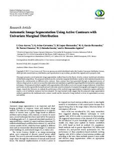
Fig. 1. Demonstration of Edgeflow vector field. a) An image of blood cells. White rectangle marks the zoom area. b) Edgeflow vectors corresponding to the zoom area.

geodesic active contours. Section V introduces Edgeflow-driven anisotropic diffusion. Section VI extends our techniques to multi-scale and in Section VII, texture segmentation is demonstrated. Section VIII describes experimental results and evaluations. We conclude in Section IX. II. P REVIOUS W ORK

ON

E DGEFLOW I MAGE S EGMENTATION [1]

The defining characteristic of Edgeflow is that the direction of the edge vectors point towards the closest edges at a predefined spatial scale in an image. An example of Edgeflow vector field is shown in Fig. 1. Assume that s = 4σ is the spatial scale at which we are looking for edges. Let Iˆσ be the smoothed image with a Gaussian of variance σ 2 . At pixel location (x, y), the prediction error along θ is defined as: ¯ ¯ ¯ˆ ¯ ˆ Error(σ, θ) = ¯Iσ (x + 4σ cos θ, y + 4σ sin θ) − Iσ (x, y)¯

(1)

This can be seen as a weighted averaged difference between the neighborhoods of two pixels and the weighting function is shown in Fig. 2(a). We define an edge likelihood in the direction θ using relative errors in the opposite directions θ and θ + π: P (σ, θ) =

Error(σ, θ) Error(σ, θ) + Error(σ, θ + π)

(2)

The probable edge direction at a point (x, y) is then estimated as: θ+π/2 Z

arg max

P (σ, θ0 )dθ0

(3)

θ θ−π/2 August 8, 2005

DRAFT

4

(a) Fig. 2.

(b)

a) Difference of offset Gaussians. The distance of the centers is determined by the scale parameter. This function is

the weighting factor used in calculating the Error(σ, θ). b) The center area is compared to the half rings 1 and 2 at all angles to find the direction of Edgeflow vectors.

This can be interpreted as comparing the weighted difference of a center area of a disk to the half rings split at a certain angle (Figure 2(b)). The weightings over this circle would approximately look like the Laplacian of a Gaussian. The edge energy along θ is defined as: E(σ, θ) = k∇θ Gσ (x, y) ∗ I(x, y)k

(4)

where ∇θ Gσ (x, y) is the derivative of Gaussian kernel at θ direction. Then the Edgeflow field is calculated as the vector sum: θ+π/2 Z ~ S(σ) = [ E(σ, θ0 ) cos(θ0 ) E(σ, θ0 ) sin(θ0 ) ]T dθ0

(5)

θ−π/2

After this vector field is generated, the vectors are propagated towards the edges. The propagation ends and edges are defined when two flows from opposing directions meet. For both x and y components of the Edgeflow vector field, the transitions from positive to negative (in x and in y directions respectively) are marked as the edges. The boundaries are found by linking the edges. Segmentation is further pruned through region merging. III. E DGEFLOW- DRIVEN C URVE E VOLUTION (EFC) Curve evolution and associated techniques were first used in other fields such as fluid dynamics before they found their applications in image processing. In [2], a general curve evolution is controlled by three separate forces: ∂C = αF1 + βF2 + F3 ∂t August 8, 2005

(6) DRAFT

5

~ is a constant expansion/shrinking force, F2 = b(x, y)κN ~ is a curvaturewhere F1 = a(x, y)N ~ ·N ~ )N ~ is a force based on an underlying vector field whose direction based force, and F3 = (S and strength is usually independent of the evolving curve. α, β are constants and C is a curve. The curve is evolved in the normal direction by a combination of these forces. a(x, y) is typically referred to as the edge function in image segmentation/curve evolution literature. Many gradientbased edge functions have been proposed in the past. In the context of image segmentation, it is ~ In the following, reasonable to closely relate edge function (a(x, y)) and the edge vector field (S). we outline our approach to computing the edge function and the edge vector field. ~ such Let us first consider the edge vector field. Note that we are interested in designing S that it guides the curve towards the region boundaries. The Edgeflow vector field discussed in Section II is a good candidate for this. An Edgeflow vector at point (x, y) is designed such that it estimates the direction towards the nearest boundary (See Fig. 1(b)). The original Edgeflow method described in Section II calculated the direction and magnitude of the vectors independently using two different techniques (Equations 3 and 4). Since we are not interested in computing the edge strength at each pixel location but rather in detecting the region boundaries, we can substitute Error(σ, θ) for E(σ, θ) in (5). This has the added advantage of significantly reduced computations. In the following discussion we use: θ+π/2 Z

~ S(σ) =

[ Error(σ, θ0 ) cos(θ0 ) Error(σ, θ0 ) sin(θ0 ) ]T dθ0

(7)

θ−π/2

As mentioned before, we would like to tightly couple the edge function and the Edgeflow vector field in evolving the curves. One choice that satisfies this condition is V (x, y) whose ~ Since Edgeflow is not necessarily a conservative vector gradient is the Edgeflow vector field S. field, we define the edge strength function as the inverse gradient of the conservative component of the Edgeflow vector field. To calculate V , we write Edgeflow as a sum of a conservative and a solenoidal vector field using the Helmholtz decomposition: ~=S ~con + S ~sol = −∇V + ∇ ~ ×A ~ S

(8)

~con is the conservative component and Ssol is the solenoidal component of S, ~ the Edgeflow where S vector field. Taking the divergence of both sides: ~ ·S ~ = −∆V + ∇ ~ · (∇ ~ × A) ~ ∇ | {z }

(9)

0 August 8, 2005

DRAFT

6

where ∆ is the Laplacian. Since the second term is zero, we only need to solve a Poisson equation [3] to find the edge function: ~ = −∆V ~ ·S ∇

(10)

To verify this solution, let us define the edge function −V as the least square solution of Z 1 ~ + ∇V k2 min E = kS (11) V 2 U where U ⊂ R2 is a bounded and open set on which the image is defined. It can be seen that E is a function of ∇V . This problem can be solved by using the first variation of E. Let us define ~ + ∇V k2 . The Euler-Lagrange equation associated with (11) is then: the Lagrangian L = 1/2kS ³ ´ ³ ´ ∂L ∂L ∂ ∂ ∂V ∂Vy x + =0 (12) ∂x ∂y where Vx = ∂V /∂x and Vy = ∂V /∂y. Derivation of this equation is given in the Appendix A. Note that L(Vx , Vy ) = 1/2(Vx + S x )2 + 1/2(Vy + S y )2 where S x and S y are the components of ~ Straight evaluation of (12) results in the same Poisson PDE (10), whose solution gives us S. the edge function V . This shows that the potential function V associated with the conservative component of Edgeflow is also the best one can achieve in the least squares (11) sense. See also [4] for a similar energy minimization approach where the inverse gradient is utilized for finding the level lines from color gradients. After scaling to the interval [0, 1], V has values around zero along the edges and values close to 1 on flat areas of the image. This edge function slows the constant expansion around region boundaries. If the curvature term is multiplied with V , this will then reduce the smoothing effect of the curvature at the edge locations, which is also desired. The Edgeflow-based curve evolution can now be formulated as: ∂C ~ ·N ~ )N ~ + V κN ~ + f (V )F N ~ = (S ∂t ~sol · N ~ )N ~ − (∇V ~ ·N ~ )N ~ + V κN ~ + f (V )F N ~ = (S

(13)

where F is a positive (negative) constant for expansion (shrinkage). We choose f (V ) = V . This discussion follows the ideas that are first proposed by Caselles et al. [5] and Malladi et al. [6]. Equation (13) can be implemented using level set methods [7, 2].

August 8, 2005

DRAFT

7

IV. C OMPARISON OF E DGEFLOW

WITH

G EODESIC ACTIVE C ONTOURS

Geodesic active contours is a standard method in edge-based curve evolution. In this section we compare Edgeflow-based curve evolution (13) with the geodesic active contours (GAC) and point out the strengths of our method. GAC is a good method to compare with because it is a widely used edge-based curve evolution method. Several variations of this method have been ~ − (∇g · N ~ )N ~ where proposed recently. The GAC formulation is given by ∂C = g(F + κ)N ∂t

g = 1/(1 + |∇Iˆσ |) and Iˆσ is the Gaussian smoothed image. This definition of g introduces a nonlinear scaling that is aimed to enhance the weak edges. This evolution is derived, excluding the constant expansion term, as the local minimization of the total curve length weighted by g. Fig. 3 compares segmentation of a simple binary image using Edgeflow and GAC. The constant expansion term is multiplied with -1 so that the curve shrinks instead of expanding. Fig. 3(d) shows that weighted curve length minimization in GAC has difficulty in handling concavities in the boundary1 . When the curve reaches a small opening in the boundary, this is a local minimum since going inside the concavity will increase the weighted curve length. On the other hand, going inside this concavity results in a better solution in the end. ~ S ~con = −∇V , S ~sol . Due to the nonlinear scaling, −∇g Fig. 4(b-d) shows the vector fields S, ˆ is displayed instead, which has a similar structure. used in GAC is not easy to visualize. ∇k∇Ik The vector fields are shown only in the neighborhood of the concavity. As can be seen, the solenoidal component of Edgeflow creates a force towards the inside of the concavity2 . Noise Sensitivity: Another important measure for curve evolution is its noise sensitivity. For this purpose, we create ten images by adding random noise to a binary image iteratively (RN is generated from RN −1 ) ten times (R1 to R10 partially shown in Fig. 5). Then, both Edgeflow and the geodesic active contours are applied to these noisy images. For each image and for each method (Edgeflow and GAC), the weighting for the constant shrinkage term is manually adjusted for best results. We observe that GAC segmentation is able to segment the object in 1

By increasing the weighting of the constant shrinkage term, the curve can be forced to evolve into the concavity. Note that

the shrinkage term does not originate from energy minimization. But in our experiments GAC strongly favors not going into the concavity and we need to find specific weightings to achieve this. Later on we will see that when noise is added, playing with the weightings of the shrinkage term will not help. On the other hand, Edgeflow naturally evolves into the concavity pretty much for any selection of weightings. 2

Advantages of using a flow consisting of a solenoidal component is also shown in [8].

August 8, 2005

DRAFT

8

(a)

(b)

(c)

(d)

Fig. 3. a) Initialization of the curve evolution. b) Segmentation result using Edgeflow. c) Segmentation using only the conservative component of Edgeflow. d) GAC segmentation

(a) Fig. 4.

~ (b) S

(c) Scon = −∇V

~ − ∇V (d) Ssol = S

ˆ (e) ∇k∇Ik

~ c) Scon = −∇V , d) Ssol = S ~ − ∇V , e) ∇k∇Ik. ˆ a) The rectangular region of interest, b) S,

images R1 to R6, and the result for R6 is shown in Fig. 6(a). In R7 to R10 the curve collapses onto itself and disappears due to boundary leaks. Edgeflow on the other hand is able to capture the object with good precision for images R1 to R8. The segmentation for R8 is displayed in Fig. 6(c). Even on R10, Edgeflow is able to capture some parts of the object demonstrating its robustness to texture. This experiment demonstrates that Edgeflow-based segmentation is more robust to noise. V. E DGEFLOW- DRIVEN A NISOTROPIC D IFFUSION (EFD) In the discussion so far, we have considered curve evolution based segmentation. Anisotropic diffusion is another important variational segmentation method. The main idea in anisotropic

August 8, 2005

DRAFT

9

(a) R1 Fig. 5.

(b) R2

(c) R3

(d) R8

(e) R9

(f) R10

(e)

(f)

a-f) Images with increasing random noise: RN = RN −1 + noise.

(a)

(b)

(c)

(d)

Fig. 6. a) R6 segmented using GAC. b) Canny edges on R6. c) R8 segmented using Edgeflow. d) Canny edges on R8. e) R10 segmented using Edgeflow. f) Canny edges on R10.

diffusion is to smooth the homogenous areas of the image while enhancing the edges, thus creating a piecewise constant image from which the segmentation boundaries can be easily obtained. Anisotropic diffusion was first proposed by Perona and Malik [9]. Perona-Malik flow can be formulated as: It = div(g∇I) with I0 being the original image. g is the edge stopping function, which allows edges below certain strength to be smoothed and stronger edges to be sharpened. An interesting work on anisotropic diffusion is self-snakes (SS) proposed by Sapiro [10]. This work uses the same partial differential equations as geodesic active contours (except the constant expansion term) but instead of evolving a single curve, each level set of the image is evolved. Self-snakes is formulated as a linear combination of a smoothing term and a sharpening term. The smoothing occurs in the tangential direction of the level sets of the image, and sharpening is applied in the orthogonal direction. The PDEs can be written as: µ ¶ ∇I It = α g div k∇Ik + β∇g · ∇I k∇Ik

(14)

where α and β are constant weighting factors. In this equation, g is defined as in the case of ³ ´ ∇I geodesic active contours and the curvature of the level sets is κ = div k∇Ik . The first term is the smoothing term and smooths the level sets of the image proportional to their curvature. The August 8, 2005

DRAFT

10

second term is used for sharpening or deblurring. In this section we propose an anisotropic diffusion framework that utilizes Edgeflow vector field for sharpening and the associated edge function V for selective smoothing. Similar to the edgeflow-driven curve evolution framework, we define our anisotropic diffusion framework as: ~ · ∇I It = αV κk∇Ik + β S

(15)

~ is the Edgeflow vector field and V is the edge function that is driven from S. ~ where S It is easy to see the similarities between the equations for self-snakes and (15). Both of these formulations are based on combining smoothing and sharpening terms and γ =

β α

defines the

tradeoff between sharpening and smoothing. On the other hand, these formulations behave very differently. Let us consider the following two extreme cases for both self-snakes and Edgeflowdriven diffusion: 1) α = 0 with β > 0, which corresponds to pure sharpening, and 2) β = 0 with α > 0, which corresponds to pure mean curvature smoothing. As demonstrated in Fig 7(a-h), if β is set to zero in self-snakes, then most boundaries are completely displaced and lost over time, which is the expected behavior of mean curvature smoothing. On the other hand, if α is set to zero, we do not expect the sharpening term to displace the boundary. Contrary to our expectations, applying self-snakes even with α set to zero (σ = 1.5), displaces the boundary and smooths it as shown in Fig 7(i-p). Edgeflow-driven diffusion does not have the same behavior (Fig. 8). In ~ and V in Edgeflow-driven flow are updated after each these examples, g in self-snakes and S iteration. The results show that self-snakes displace the edges. This effect of displacement is more severe with increasing scale. A. Edgeflow on Color Images Our discussion so far is based on brightness features of the image. A common approach [11] to extending anisotropic diffusion techniques to color images is to derive the vector field, edge function, and the color gradients using all three color components, and then apply diffusion to each color component separately. In our method, these three diffusions are coupled through the Edgeflow vector field and the edge function. For this purpose we need definitions of Edgeflow vector field and the gradient on vector valued images since color features can be thought of as three dimensional vectors at each pixel.

August 8, 2005

DRAFT

11

(a) 0 iterations

(b) 500 iterations

(c) 2000 iterations

(d) 4000 iterations

(e) 0 iterations

(f) 500 iterations

(g) 2000 iterations

(h) 4000 iterations

(i) 0 iterations

(j) 500 iterations

(k) 2000 iterations

(l) 4000 iterations

(m) 0 iterations

(n) 500 iterations

(o) 2000 iterations

(p) 4000 iterations

Fig. 7. Self-snakes image diffusion. First two rows correspond to the diffusion and edge function g for the case when β is set to zero. Third and forth rows correspond to the diffusion when α is set to zero.

A derivation of gradient for vector-valued images is given by Di Zenzo [12]. Let I~ = [I 1 . . . I N ]T : R2 → RN be a vector-valued image.  I~x · I~x M = I~x · I~y

Define a 2 × 2 matrix M as:  ~ ~ Ix · Iy  ~ ~ Iy · Iy

(16)

where I~x and I~y are the derivatives of I~ with respect to x and y. Let ~v be a unit vector at direction θ. The directional derivative of I~ = [I 1 . . . I N ]T at the direction ~v is given as: ~ y))2 = ~v T M~v (∇θ I(x,

(17)

Then the gradient magnitude and direction are given by the square root of larger eigenvalue August 8, 2005

DRAFT

12

(a) 0 iterations

(b) 500 iterations

(c) 2000 iterations

(d) 4000 iterations

(e) 0 iterations

(f) 500 iterations

(g) 2000 iterations

(h) 4000 iterations

Fig. 8. Edgeflow-driven image diffusion for α = 0. First row shows the diffusion process and the corresponding edge functions V are given in the second row.

of M and the corresponding eigenvector. In our algorithms, this gradient is used for finding boundaries after diffusion converges. To be able to conduct the anisotropic diffusion process on color images we also need a definition of Edgeflow for vector-valued images. Ma and Manjunath [1] extended Edgeflow to color and texture images by finding the prediction error for each feature component and combining them by summation. We suggest a different approach by using the definition of the directional derivatives for vector-valued images (17). By rearranging terms, (17) can be rewritten as: °h ° ~ ∇θ I(x, y) = ° I~x

° ° ° ∇θ I 1 ° i ° ° ° ~ Iy ~v ° = ° : ° 2 ° ° ∇θ I N

° ° ° ° ° ° ° ° °

(18) 2

Similarly, by using the result from (18) the prediction error for a vector-valued image at the direction θ can be defined as:

° ° ° Errorθ I 1 ° ° Error(σ, θ) = ° : ° ° ° Errorθ I N

° ° ° ° ° ° ° ° °

(19) 2

This result shows that the prediction error for a vector-valued image is the L2 norm of a vector created by the prediction errors of individual feature components. Original Edgeflow method has

August 8, 2005

DRAFT

13

extended error calculation to vector-valued images in a similar way but using L1 norm instead of L2 norm, which turns out to be an approximation of (19). VI. M ULTI - SCALE A NISOTROPIC D IFFUSION To extend our anisotropic diffusion technique to multi-scale segmentation, we only need to modify the design of the Edgeflow vector field. Edge function and the PDE’s for anisotropic diffusion would stay the same. Our main goals in designing the multi-scale Edgeflow vector field are: 1) Localize edges at the finer scales. 2) Suppress edges that disappear quickly when scale is increased. These are mostly spurious edges that are detected at the fine scale because of noise and clutter in the image but do not form salient image structures. 3) Favor edges or edge neighborhoods3 that exist at both fine and coarse scales. In generating our vector field, we will explicitly use a fine to coarse strategy. On the other hand, our multi-scale framework also conducts coarse to fine edge detection implicitly. Take s1 as the finest (starting) scale and s2 as the coarsest (ending) scale. We are interested in analyzing an image between scales s1 and s2 for finding the edges. The algorithm for generating the multi-scale Edgeflow vector field is given in Algorithm 1. As can be seen, the vector field that is generated at scale s1 is selectively updated using the vector fields from coarser scales. The vector field update procedure can be interpreted as follows: At a finer scale, the vector field only exists on a thin line along the edges. Therefore, within the homogenous areas the vectors are of zero length. With increasing scale the reach–coverage area–of the vector field also gets thicker. First of all, we want to preserve the edges detected at the fine scale, which implies that we preserve strong vectors from the fine scale. We also would like to fill the empty areas with vectors from larger scales. The main reason for this is that some edges that do not exist at fine scales, the so called shadow, shading or blur edges, ~ y)k < M , and if so, will be captured at the coarser scales. For these reasons, we check if kS(x, C

fill this pixel with a vector from a larger scale. Note also that the proposed method favors edges that exist at multiple scales and suppress edges that only exist at finer scales. If the vector directions match at multiple scales, this means 3

For larger scales, edges are displaced from their original locations. For this reason, it makes more sense to discuss edge

neighborhoods when coarser scales are considered.

August 8, 2005

DRAFT

14

Algorithm 1 Algorithm for generating a multi-scale Edgeflow vector field. Let I(x, y) be the image. Let C be a positive constant (e.g. 15). Let A be a positive constant corresponding to an angle (e.g. π/4). Let s1 be the smallest and s2 be the largest spatial scale at which we are interested in analyzing the image for edges. Let ∆s = 0.5 pixel be the sampling interval for the scale. ~ at scale s = s1 . From I, calculate the initial vector field S while s < s2 do Set s = s + ∆s. Calculate Edgeflow vector field T~ at scale s. ~ M = M ax(kSk) for all Pixel (x, y) in I do ~ y)k < M then if kS(x, C

~ y) = T~ (x, y) S(x, ~ y) and T~ (x, y) is less than A then else if The angle between S(x, ~ y) = S(x, ~ y) + T~ (x, y) S(x, else ~ y) is kept the same. S(x, end if end for end while ~ gives the multi-scale Edgeflow vector field. The final S

that the edges exist at multiple scales. Based on this observation, we check the vector directions from larger and finer scales and if they match, we sum the vectors up to strengthen the edge. Another possibility is that the edge is shifted from its original location at the coarser scale. In that case, the vector at the pixel that is in between the original (finer scale) edge and the shifted (coarser scale) edge will change its direction by 180 degrees. As we discussed before, we favor the edge localization at the finer scale. Therefore the new vector from the coarser scale

August 8, 2005

DRAFT

15

Fig. 9.

(a)

(b) σ = 1

(c) multi-scale

(d) σ = 4

Demonstration of multi-scale edge detection. a) Original image. Color image is shown but gray scale intensities are

used in edge detection. b) Edge strength at spatial scale σ = 1 pixel. c) Multi-scale edge detection using scales from σ = 1 to σ = 4. d) Edge strength at scale σ = 4 pixels.

is ignored and the vector from the finer scale is preserved. Figure 9 shows the results of multi-scale edge detection (using gray-scale intensities) image with s1 = 1, s2 = 4, ∆s = 0.5, C = 15, and A = π/4. The strength of the edges are represented by the sum of strengths of the vectors at the edge location where the vector field changes its direction. Multi-scale edge detection results are compared to edge detection results at σ = 1 and σ = 4. These results show that the results corresponding to σ = 1 localizes edges very well but detect clutter and noise as edges. The results corresponding to σ = 4 include cleaner results but the edges are not well localized (See the tail of the fish in Figure 9d). On the other hand, by combining results from scales 1 to 4, we are able to achieve edge detection results that both localize edges precisely (as in σ = 1) and create a cleaner edge detection (as in σ = 4). Fig. 10 demonstrates the behavior of the multi-scale segmentation compared to segmentations at the fine and coarse scales. The results show that using a multi-scale approach we are able to August 8, 2005

DRAFT

16

(i) Fig. 10.

(a)

(b) σ = 1.5

(c) σ = 6

(d) multi-scale

(e)

(f) σ = 1.5

(g) σ = 6

(h) multi-scale

(j) σ = 1.5

(k) σ = 6

(l) multi-scale

(m) σ = 6

(n) multi-scale

Color images are shown but gray scale intensities are used in segmentations. a) Original image. b) Segmentation

result at spatial scale σ = 1.5. c) Segmentation result at σ = 6. d) Multi-scale segmentations using scales σ = 1.5 to σ = 6. e) Original image. f) Segmentation result at σ = 1.5. g) Segmentation result at σ = 6. h) Multi-scale segmentations using scales σ = 1.5 to σ = 6. i) Detail around the head area. j) Detail for σ = 1.5 k) Detail for σ = 6 l) Detail for multi-scale segmentation. m) Detail around head area for σ = 6. n) Detail for multi-scale segmentation.

capture salient structures from a range of scales. It is to be noted that region merging using fine scale segmentation will not usually give the similar results as our multi-scale segmentation. For example, in Figures 10 (b-d), there are certain boundaries and structures that emerge as the scale increases and these boundaries are not captured or do not exist at the smaller scales. Figures 10 (i-l) demonstrate the excellent edge localization property of our multi-scale algorithm. Fig. 10 (e-h) show another example of a multi-scale segmentation and shows the better localization of the edges around the head area using multi-scale approach compared to segmentation at scale σ = 6. VII. T EXTURE S EGMENTATION USING A NISOTROPIC D IFFUSION Texture is an important visual image feature and utilizing texture within the image segmentation process in general is desired. Previous work on texture-based anisotropic diffusion [13, 10]

August 8, 2005

DRAFT

17

utilized filter outputs generated by convolving the image with a set of Gabor filters. As opposed to gray-scale intensities or color features, texture is not a point-wise feature. Filter outputs not necessarily represent textures by themselves and usually are not homogenous within the same texture. Given a small window within which a texture is visible, distribution of filter outputs within this window form a representation of this texture. Various methods for generating texture features from filter outputs has been proposed. Commonly, filter outputs are clustered using k-means [14] or Gaussian mixture models (GMM) [15] to generate codewords, which are called textons. In this section, we use a rotation insensitive Gaussian mixture model to learn the textons as proposed by Newsam et al. [16]. Our texture features at each pixel are the histograms of rotation insensitive textons within a square window centered at each pixel [17]. These histograms, which are high dimensional feature vectors, can be calculated very efficiently–pretty much real time–with O(N ) complexity (N is the total number of image pixels) by utilizing cumulative sums. Edgeflow vector field on these texture feature vectors is calculated same way as in the color case described in Section V-A. Figure 11 demonstrates texture segmentation on an aerial image of size 2048x2048. Image is filtered with Gabor filters at 5 scales and 6 orientations. Design of the Gabor filters follow Manjunath and Ma [18] with UL = 0.05 (roughly corresponds to a filter support of 75x75) and UH = 0.4 (roughly corresponds to a filter support of 11x11). 200,000 points are sampled from the filter outputs and a Gaussian mixture model is created with 10 Gaussians and pixels are mapped to one of these Gaussians (textons) (See Fig. 11 m). As can be seen, rows of boats that are oriented in different directions within harbors have similar texton distributions. Then, in 100x100 windows centered at each pixel, histograms of 10 bins are created (See figures 11(c-l)) Anisotropic diffusion is conducted after subsampling the histograms to 250x250 for computational efficiency. Scale is selected as σ = 2 pixels. Segmentation result shows that texture-wise homogenous objects such as harbors, urban areas, highways, etc. are correctly segmented. The segmentation boundaries are not as precise as in the case of gray scale but this is essentially because texture is visualized in 100x100 windows, which introduces location uncertainty. Note that obvious gray scale edges may not correspond to texture edges. Local distributions of texton labels in Fig. 11 m) would help with the visualization of textures and fine resolution micro textures of harbors are shown in in Fig. 11 m). Fig. 12 shows texture segmentation on an image of a zebra. Image is of size 294x178. This August 8, 2005

DRAFT

18

(a)

(c)

(d)

(m) Fig. 11.

(e)

(b)

(f)

(n)

(g)

(h)

(i)

(o)

(j)

(k)

(l)

(p)

Texture segmentation using anisotropic diffusion on rotation insensitive texton histograms. a) Original image. b)

Segmentation result. c-l) Texton frequencies (histogram bins). m) Detail showing the micro textures on the aerial image after zooming in. n) Texton labels shown in pseudo-color (best viewed in color). o) Edge function V generated from Edgeflow vector field. p) Gradient of the diffused (multi-valued) image.

image is analyzed at 4 scales and 6 orientations and only 5 textons are generated and segmentation is conducted with σ = 3. As can be seen, number of textons needed are very small due to the rotation insensitivity of our textons, which is important for the feasibility and efficiency of the anisotropic diffusion process. Note that, in this section gray scale intensities are not used directly. In the next section we evaluate gray scale intensities and color features within our segmentation framework. August 8, 2005

DRAFT

19

(a)

(c)

(d)

(h) Fig. 12.

(b)

(e)

(i)

(f)

(g)

(j)

Texture segmentation using anisotropic diffusion on a zebra image. a) Original image. b) Segmentation result. c-g)

Texton frequencies (histogram bins). h) Texton labels. i) Edge function V generated from Edgeflow vector field. j) Gradient of the diffused (multi-valued) image.

VIII. E XPERIMENTS : M ODEL S ELECTION AND P ERFORMANCE E VALUATION In the past, quality of segmentation results are generally evaluated visually and shown on a limited set of images. Recently introduced Berkeley Segmentation Data Set and associated ground truth [19] offers an excellent opportunity to have a well defined learning and evaluation framework for image segmentation. In our experiments, we optimize and compare three edgebased curve evolution techniques and three anisotropic diffusion techniques on natural images using Berkeley Segmentation Data Set. The curve evolution techniques we evaluate are: geodesic active contours (GAC) from Caselles et al. [20], gradient vector flow (GVF) from Xu and Prince [8], and Edgeflow-driven curve evolution (EFC) we introduced in Section III. Anisotropic August 8, 2005

DRAFT

20

diffusion techniques we evaluate are: Perona-Malik flow (PM) [9], self-snakes (SS) from Sapiro [10], and Edgeflow-based anisotropic diffusion (EFD) we introduced in Section V. We chose these techniques in our evaluations due to their popularity. It is true that more recent and many variations of these techniques have been proposed in the literature. Our evaluations provide a baseline for more recent methods. For example [21], [22], and [23] criticized certain aspects of GVF and suggested modifications to the vector field generation and curve evolution process. We are making our evaluation software available on the web so that these techniques can also be evaluated. A. Berkeley Segmentation Data Set (BSDS) The experiments for the evaluation are conducted on Berkeley segmentation data set. The data set is divided into two sets: training and test sets. The suggested training set consists of 200 images and the test set consists of 100 images. The idea is to optimize all the parameters of your algorithm on the training set and then the evaluation is done on the test set. We randomly selected the following 20 images for training (due to computational reasons): 181091, 55075, 113009, 61086, 65074, 66075, 170054, 164074, 118020, 145014, 207056, 247085, 249087, 35091, 41025, 45077, 65019, 97017, 76002, 80099. Visually, the images in our training set seem to be diverse. The test set is kept the same (100 images). The original images are of size 481x321. Again, due to computational reasons, for curve evolution experiments we resize these images to 192 × 128 and for anisotropic diffusion the images are resized to 240 × 160 (In [24], the images are also resized for computational reasons). The segmentations are matched to the ground truth by following the same methodology used in [24]. We conducted our experiments in this paper using both gray scale and color values of the images. The Berkeley segmentation data set provides two sets of ground truth, one generated by displaying color images and the other by displaying gray-scale versions to the subjects. Previous work use gray scale ground truth for evaluating methods that are based on gray scale intensities (or texture) and color ground truth for methods that utilize color information. Considering that we compare both gray scale and color segmentation results in this paper, we choose to use higher quality ground truth, from color images, in our evaluation.

August 8, 2005

DRAFT

21

B. Optimizing Curve Evolution We can formulate a generic edge-based curve evolution with the following PDE:

∂C ∂t

= αF1 +

βF2 + F3 where F1 is the term for constant expansion weighted by an edge function, F2 is the curvature-based force, and F3 is the vector field based force. There are three parameters that directly affect the curve evolution, α, β and the scale σ at which the edge function and the vector field are generated. β, the weighting factor for the curvature-based term adjusts the smoothness of the curve during its evolution. If β is adjusted to a reasonable value, variations in β will not have a significant effect on the final segmentation. Reasonable value for beta is decided such that the curve is flexible and smooth during the evolution. We fine tune β manually on each curve evolution technique to a reasonable value and visually keep the effect of the curvature same for each method we are testing. The training phase requires finding the optimum values of α and σ for each of the curve evolution techniques. We utilize combinatorial optimization for the optimization of these two parameters. The scale σ is directly linked with the edge detection and edge localization quality. A key behavior of the curve evolution is that the constant expansion term (F1 ) competes with the vector field (F2 ) in the curve evolution framework. If α is selected too high, the curve will not stop at the edges, and if α is too low, the curve might not reach the boundary. Given a scale σ, we first generate the edge function and the vector field. Then, a useful range of values for α is identified. The range of values for α should start from a low value which is not high enough to carry the curve to the boundaries (e.g. 0) to a high value for which the curve does not stop at any edge point. This interval for α depends on the curve evolution technique, but it does not change from one scale to another in our experiments. Once we decide on the interval for α, this interval is sampled at equally spaced points. For each of these values of α, the curve evolution and the associated segmentation are generated. A measure of goodness of segmentation is needed to compute the optimal value of α. In [24], a way to match a segmentation to the ground truth and calculating precision and recall for the match is proposed. Thinned edges are matched to the ground truth and based on this match, precision (P) and recall (R) are calculated. To define a single goodness measure from precision and recall, the F-measure has been used: F =

P ·R , ξP +(1−ξ)R

where ξ defines the tradeoff

between precision and recall. In [24], ξ is selected as 0.5, which we also follow. For better

August 8, 2005

DRAFT

22

(a) Fig. 13.

(b)

(c)

Curve instantiation setup. a) A multi-part curve, b) 4 multi-part curves each with 4 sub-parts, c) 9 curves total: 4

multi-part curves and 5 single-part curves.

resolution, successive samples of α, αn and αn+1 are interpolated and P and R are estimated by linear interpolation using the P and R values at αn and αn+1 . Finally, the value of α with the highest F-measure is selected as the optimum for this scale. This process is repeated for a range of scales and the scale with the highest F-measure is selected as the optimum scale. Based on our experiments, a difference of 0.01 in F-measure corresponds to visual improvements in segmentation quality. Curve evolution methods are usually intended to capture a single object boundary. For our evaluation framework we need to create a full segmentation. For this purpose, we propose using multiple curves. Four multi-part curves, each with four sub-parts and five single-part curves (total of nine curves) are initialized on the image in a grid fashion (See Fig. 13). We need to note that each extra curve adds to the computational complexity and therefore it is not practical to use a large number of curves. To decide if a curve has converged or not, we need to define a convergence criterion. Our convergence criterion is closely linked with our implementation of the curve evolution. In this work, curve evolution is implemented using narrow band level set methods [2]. We take the narrow band size as six pixels. If the curve stays within this narrow band for a large number of iterations (we choose this number to be 60), we conclude that the curve has converged. As a failsafe, after 8000 iterations the curve is stopped regardless. 1) Training Geodesic Active Contours (GAC): By the design of GAC, the range of edge stopping function g is nonlinearly scaled between 0 and 1. By visual inspection, we set β (weighting factor for the curvature-based term) to 0.3, and the range of α is chosen from 0.1 to 1 with increments of 0.1. The performance peaks at σ = 0.75 (F = 0.559) with α = 0.3.

August 8, 2005

DRAFT

23

2) Training Gradient Vector Flow (GVF): Gradient Vector Flow (GVF) defines a method of generating a vector field. Given an edge strength function f (x, y) of the image (for example ~ is realized as the minimization of an energy functional. f (x, y) = k∇Ik), this vector field G Matlab source code for calculating GVF has been provided by its authors on their web site, which we follow in our implementation. The decisions for parameter settings are done based on the suggestions of the authors in their paper [8] and in their source code. µ is set to 0.1 and the √ number of iterations is set to N M where N is the width and M is the height of the image. The curve evolution setup for GVF is exactly same as the one for GAC except that the edge stopping function and the vector field are different. The edge strength function is selected as f = k∇Ik and f is linearly scaled to the interval [0, 1]. Edge stopping function is calculated as g = −f + 1. β is visually set to 0.003, and the range of α is from 0 to 0.1 with increments of 0.01. The performance peaks at σ = 1.25 for α = 0.02 (F = 0.506). The performance of GVF is much lower than GAC on the training set (0.51 vs 0.56). The vector field for GVF works well as expected when there are clear step edges in the image. On more complex images (which have weak edges along the boundary and clutter) and for small scales (for which ∇f might be thin along the edges), GVF is not able to interpolate the vector field as well. 3) Training Edgeflow (EFC): Considering that the design of EFC is not fixed like GAC or GVF, while we optimize EFC, we also test different design decisions using the training set. The first decision we need to make is about the scaling and the dynamic range of the edge function ~ One option is to scale them independently, and the other option is V and the vector field S. to scale them together by the same factor. We investigate both these options. First we conduct ~ are both linearly the experiments for independent scaling. Values of V and magnitudes of S scaled to the interval [0, 1]. Then both of them are divided by their means for normalization. For this setup we select β as 0.3 and the range of α is set as 0.1 to 1 with increments of 0.1. The performance peaks at σ = 0.5 and α = 0.2 (F = 0.561). An interesting observation about these results is that EFC’s performance falls rapidly with respect to scale increase. The problem originates from the use of Gaussian offset at 4σ when creating difference of offset Gaussians (DOOG) filters. This large Gaussian offset introduces poor localization in EFC with increasing scale. Based on this observation, we redesign a new Edgeflow vector field using a Gaussian offset of σ. We call this vector field and the associated curve evolution as EFC2. EFC2 has a better performance (F = 0.564) and the performance is August 8, 2005

DRAFT

24

0.6

EF’ EF2’

F−Measure

0.55

GAC 0.5

GVF

0.45

0.4

0.35

0

0.5

1

1.5

2

2.5

3

3.5

4

Smoothing Scale

Fig. 14.

Performance comparison of EFC0 , EFC20 , GAC and GVF on the training set.

stable across a wide range of scales. We repeat the experiments for EFC and EFC2 by scaling the edge function V and the vector ~ in a dependent way. Let m = M in(V ) and M = M ax(V ). We subtract m from V field S ~ are divided by to make the minimum 0. After that both V and x and y components of S ~ by 20 so that α and β parameters can be kept same. We call the M − m. Then we multiply S corresponding curve evolutions EFC0 and EFC20 . Dependent scaling improves the performance (F = 0.566 for EFC0 and F = 0.573 for EFC20 ). Fig. 14 shows the training results for EFC0 , EFC20 , GAC and GVF. 4) Test results: We apply curve evolution techniques we trained so far to the test set of 100 images associated with the Berkeley segmentation data set. For edgeflow, we test both EFC0 and EFC20 . A summary of the optimum values that are calculated form the training set, the performance on the training set, and the performance on the test set are provided in Table I. GVF perform worse than other techniques as expected based on the training phase. The results show that both EFC0 and EFC20 show about 0.02 improvement with respect to GAC. More importantly EFC20 is less sensitive to scale changes and performs quite well over a large range of scales.

August 8, 2005

DRAFT

25

Technique

σ

α

β

F (training)

F (test)

GAC

0.75

0.3

0.3

0.559

0.511

GVF

1.25

0.02

0.003

0.506

0.474

0.75

0.3

0.3

0.566

0.525

1.5

0.3

0.3

0.573

0.526

EFC

0

EFC2

0

TABLE I S UMMARY OF THE OPTIMUM VALUES FOR CURVE EVOLUTION

C. Optimizing Anisotropic Diffusion We evaluate and compare three anisotropic diffusion techniques: Perona-Malik flow (PM), selfsnakes (SS), and Edgeflow-driven anisotropic diffusion (EFD or EF2D depending on the Gaussian offset). EFD and EF2D use same Edgeflow vector fields as EFC0 and EFC20 as defined in Section VIII-B.3. We evaluate each technique both using gray scale intensities and also using CIE-L*a*b* color space. The evaluation framework in principle follows the framework introduced in Section VIII-A. We need to run each of these diffusion techniques until their convergence. Instead of using a heuristic method to check convergence, we decided to let each diffusion to run 5000 iterations for segmentations using gray-scale intensities and 1500 iterations for segmentations using color features. This many iterations are almost always enough for these diffusion techniques to converge. 1) Training Perona-Malik Flow (PM): Matlab source code for PM (for a gray scale image) has been provided by its authors in [25, Chapter 3]. This code uses exponential nonlinearity for the edge stopping function. Since this is the implementation favored by its authors, we will directly follow this code in our experiments. For completeness we reproduce the source code in Appendix B. Color segmentations utilize Di Zenzo’s [12] definition for gradients of multi-valued images and follow the suggested implementation of Sapiro and Ringach [11]. The parameter K works like a threshold for edge strength. For small K, more edges are preserved and for large K only strong edges are preserved. In our experiments we set K from 1 to 10 with increments of 1 for gray scale and 0.5 to 5 with increments of 0.5 for color. The optimum value for K is estimated using precision, recall and F-measure as described in the

August 8, 2005

DRAFT

26

curve evolution section. The range of K is chosen such that for smallest K, unreasonably large number of pixels of the image are labeled as the edges and for largest K most of the edges of the image are missed. There is no scale to adjust in PM so K is the only parameter to tune. Perona-Malik flow was originally demonstrated for edge detection. On the other hand, when anisotropic diffusion converges, one can actually obtain a proper segmentation for which the contours are closed. To generate the segmentation boundary from the diffused images, we propose the following: •

First let the anisotropic diffusion run for 5000 iterations. At the end, this diffusion results in a piecewise homogenous image Id (x, y).

•

To extract the boundaries from Id , calculate the gradient magnitudes f (x, y) = k∇Id k. To identify boundary and non-boundary points, f needs to be thresholded. If the histogram of f is visualized, it can be seen that there are two peaks, one around 0, which corresponds to non-boundary points, and the second group is around c, where c > K. This group corresponds to boundary points. The ideal threshold turns out to be the point right after the end of the first lump. Anything smaller causes large chunks of homogenous areas to be labeled as edges and any higher threshold causes legitimate edge points to be missed. This threshold we described is equal to K. This is expected since Perona-Malik flow sharpens edges stronger than K while smoothing out other edges.

•

Threshold f at K. This results in a binary segmentation B1 (x, y), but at this point the boundaries are not as thin as we want them. In our evaluation framework, edge localization is very important.

•

Apply standard non-maxima suppression to f using the gradient orientations and then threshold it at K. This results in another binary image B2 (x, y). The boundaries are thinned as we wanted but they are not always closed anymore.

•

From B1 , find and label connected non-boundary regions. Let us call these regions Ri where i = 1 to N . We would like to grow these regions until the boundaries are thinned and are 8-connected.

•

Identify the set of boundary points b1 from B1 and b2 from B2 . For each Ri , identify the points that are on the boundary of Ri . Grow each of Ri outwards iteratively. The rules for region growing are as follows.

August 8, 2005

DRAFT

27

Anisotropic Diffusion

Image

Diffused Image Id

Gradient

f(x,y) Non-maxima Suppression Threshold Threshold

B1

b1

Ri

B2

b2

Region Growing

Fig. 15.

Final Boundaries

Flowchart of the algorithm for capturing thin boundaries from piecewise homogenous diffused image, generated by

anisotropic diffusion.

– First grow the regions only towards the boundary points that are in the set b3 = b1 \ b2 . It is ideal for the final boundaries to include the non-maxima suppressed edges, b2 , as much as possible. Identify combined set of points that are on the boundary of all Ri and that are an element of b3 and that are not 4-neighbors of more than one region. Sort these points based on their gradient strength f (x, y). Grow regions starting with the point that has the smallest f value. For each pixel, check to see if it still neighbors with only one region. If not, don’t grow the region to this pixel. After the first iteration of region growing, find the new boundary points of Ri and continue growing until convergence. – Repeat the region growing step described in the previous step but take b3 = b1 . •

After the convergence of the last step, we obtain a proper segmentation with thinned boundaries as desired. This process can be easily and very efficiently implemented.

A flowchart for this algorithm is presented in Fig. 15. Experiments on the training set of 20 images show that the optimum value of K is 3.67 with August 8, 2005

DRAFT

28

a performance of 0.551 on gray scale images and 1.59 with a performance of 0.610 on color images. A general observation from these experiments is that noise and clutter result in poorly fragmented image segments for PM. 2) Training Self-Snakes (SS): As we discussed in Section V, SS has a problem with displaced and smoothed boundaries. For scales larger than σ = 1, the boundaries are completely out of sync with the image. Based on this perspective, we only evaluate SS at scales σ = 0.25,0.50,0.75,1. At each scale, we vary γ =

β α

to find the optimal point. The segmentation boundaries are generated

same as PM and the threshold is set to 1. The optimum scale for gray scale images is 0.25 with the performance of F = 0.505 for γ = 0.97. For color images, optimum scale is 0.25 with a performance of F = 0.567 for γ = 2.5. 3) Training Edgeflow: We investigated various design decisions regarding Edgeflow in Section VIII-A when we evaluated curve evolution. We found that EFC0 and EFC20 gave the best performance. We define EFD and EF2D for anisotropic diffusion based on the same vector ~ and edge function V as in EFC0 and EFC20 . field S During the diffusion process, ideally, Edgeflow vector field and the edge function V are regenerated after each iteration. Unfortunately this introduces extra computational burden. Instead we choose to calculate Edgeflow only once at the beginning and reuse it. In our experiments, not updating Edgeflow iteratively did not cause performance degradation. After applying (15) to an image, a piecewise homogenous image, Id is obtained. To further enhance the edges, we also apply PM with K=1 to Id right before we generate the boundaries. Since K is chosen very low, all the regions captured by (15) are preserved. Fig. 16 shows the performances of EFD, EF2D, SS, and PM on gray scale images. EF2D performs better and peaks at σ = 1 for γ = 1.0 (F = 0.612). EFD’s peak performance is at σ = 0.5 for γ = 1.15 (F = 0.599). Fig. 17 shows the performances of EFD, EF2D, SS, and PM on color images. Both EFD and EF2D perform quiet well (F = 0.704) compared to self snakes and Perona-Malik flow. EFD’s peak performance is at σ = 0.5 for γ = 1.0 and EF2D’s peak performance is at σ = 1.25 for γ = 0.7. Again EF2D shows a very stable performance across a wide range of scales. 4) Test results: A summary of performance results for both gray scale intensities and color features on the test set of 100 images is given in Table II. EFD and EF2D clearly outperform both SS and PM. These results are also much better than the results we obtained using curve August 8, 2005

DRAFT

29

EF2D

0.6

Perona−Malik

F−Measure

0.55

EFD

0.5

Self Snakes

0.45

0.4

0.35

0.3

0

0.5

1

1.5

2

2.5

3

Smoothing Scale

Fig. 16.

Performance comparison of EFD, EF2D, PM and SS on the training set using gray scale images.

Gray Scale Images

Color Images

Technique

σ

γ

F (training)

F (test)

Technique

σ

γ

F (training)

F (test)

PM

N/A

N/A

0.551

0.513

PM

N/A

N/A

0.610

0.556

SS

0.25

0.97

0.505

0.476

SS

0.25

2.5

0.567

0.537

EFD

0.5

1.15

0.599

0.569

EFD

0.5

1.0

0.704

0.627

EF2D

1

1.0

0.612

0.565

EF2D

1.25

0.7

0.704

0.626

TABLE II S UMMARY OF THE OPTIMUM VALUES FOR ANISOTROPIC DIFFUSION

evolution. Fig. 18 shows segmentation results for PM, SS, EFD and EF2D on a test image. These results are obtained using gray scale intensities. Color segmentation results for EFD on the test set using the estimated parameters are shown in Figure 19. If desired, these results can be further improved by applying simple post-processing such as region merging.

August 8, 2005

DRAFT

30

0.75

EF2D

EFD

0.7

0.65

Perona−Malik

F−Measure

0.6

0.55

Self Snakes

0.5

0.45

0.4

0.35

0.3

0

0.5

1

1.5

2

Smoothing Scale

Fig. 17.

Performance comparison of EFD, EF2D, PM and SS on the training set using color images.

D. Discussions Both Edgeflow-driven curve evolution and anisotropic diffusion proposed in this paper show promising results. On the other hand, one would have expected a better performance from Gradient Vector Flow and Self-Snakes. In Gradient Vector Flow, we observed that strong edges dominated and eliminated the nearby weak edges during vector field extension stage and caused large openings on the boundary. This is more of a problem on natural images where texture and clutter result in many weak edges. There are two main observations with Self-Snakes: 1) the image is in general oversegmented and 2) the boundaries are smoothed and displaced for larger scales. Note that it is possible to improve the segmentation performance of Self-Snakes by applying region merging as a postprocessing step. Since we wanted to avoid heuristics in our evaluations, we didn’t do this. Segmentation results for each method and evaluation software, which is used to generate results in our experiments, can be obtained from the UCSB Vision Research Lab web site at http://vision.ece.ucsb.edu.

August 8, 2005

DRAFT

31

(a) PM

(b) SS

(c) EFD

(d) EF2D

Fig. 18. Anisotropic diffusion comparison on a test image using optimum parameters learned on training set. Images are shown in color but segmentations are generated from gray-scale values. a) Segmentation using Perona-Malik flow, b) segmentation using self-snakes, c) segmentation using EFD and d) segmentation using EF2D.

IX. C ONCLUSION In this paper we introduced and evaluated robust variational segmentation techniques–curve evolution and anisotropic diffusion–that are driven by an Edgeflow vector field. We have shown that our techniques work well on natural images, which are rich in texture and clutter. We designed a common evaluation framework for edge-based curve evolution and anisotropic diffusion. To the best of our knowledge, this is one of the first evaluation of variational segmentation on Berkeley Segmentation Data Set. Our evaluations show that Edgeflow-based variational methods outperform some of the well known variational techniques on natural images. The evaluations are done using both gray scale intensities and CIE-L*a*b* color space. One of the useful result of our experiments is that we estimated specific parameters that can be easily utilized in practical segmentation applications.

August 8, 2005

DRAFT

32

Fig. 19.

EdgeFlow (EFD) results on the test set using color features. (Images are best viewed in color)

Acknowledgements We thank Daniela Ushizima Sabino, Charless Fowlkes and Dr. David Martin for their help with the setup of Berkeley Segmentation Data Set and Dr. Chenyang Xu for providing GVF matlab source code. Our colleague Sitaram Bhagavathy provided the software and helped us with the creation of texton histograms. We also would like to thank Prof. Shiv Chandrasekaran, Dr. Charles Kenney, and Marco Zuliani for fruitful discussions. This work is supported by the August 8, 2005

DRAFT

33

National Science Foundation award NSF ITR-0331697. R EFERENCES [1] W.-Y. Ma and B. S. Manjunath, “Edgeflow: a technique for boundary detection and image segmentation,” IEEE Transactions on Image Processing, pp. 1375–88, August 2000. [2] J. A. Sethian, Level set methods and fast marching methods: evolving interfaces in computational geometry, fluid mechanics, computer vision, and materials science, Cambridge University Press, 1999. [3] L. C. Evans, Partial Differential Equations, American Mathematical Society, June 1998. [4] D. H. Chung and G. Sapiro, “On the level lines and geometry of vector-valued images,” IEEE Signal Processing Letters, pp. 241–243, September 2000. [5] V. Caselles, F. Catte, T. Coll, and F. Dibos, “A geometric model for active contours in image processing,” Numerische Mathematik, pp. 1–31, 1993. [6] R. Malladi, J. A. Sethian, and B. C. Vemuri, “Evolutionary fronts for topology-independent shape modeling and recovery,” in European Conference on Computer Vision (ECCV), 1994, pp. 3–13. [7] S. Osher and J. A. Sethian, “Fronts propagating with curvature-dependent speed: Algorithms based on hamilton-jacobi formulations,” Journal of Computational Physics, 79:12–49, 1988. [8] C. Xu and J. L. Prince, “Snakes, shapes, and gradient vector flow,” IEEE Transactions of Image Processing, pp. 359–69, March 1998. [9] P. Perona and J. Malik, “Scale-space and edge detection using anisotropic diffusion,” IEEE Transactions on Pattern Analysis and Machine Intelligence, pp. 629–639, July 1990. [10] G. Sapiro, “Vector (self) snakes: a geometric framework for color, texture, and multiscale image segmentation,” in IEEE International Conference on Image Processing (ICIP), 1996, pp. 817–20. [11] G. Sapiro and D. Ringach, “Anisotropic diffusion of multivalued images with applications to color filtering,” IEEE Transactions on Image Processing, pp. 1582–1586, November 1996. [12] S. D. Zenzo, “A note on the gradient of a multi-image,” Computer Vision, Graphics and Image Processing, pp. 402–407, 1986. [13] Y. Rubner and C. Tomasi, “Coalescing texture descriptors,” in ARPA Image Understanding Workshop, February 1996. [14] T. Leung and J. Malik, “Recognizing surface using three dimensional textons,” in International Conference on Computer Vision (ICCV), 1999. [15] S. Bhagavathy, S. Newsam, and B. S. Manjunath, “Modeling object classes in aerial images using texture motifs,” in International Conference on Pattern Recognition (ICPR), August 2002. [16] S. Newsam and B. S. Manjunath, “Normalized texture motifs and their application to statistical object modeling,” in CVPR Workshop on Perceptual Organization in Computer Vision, Jun 2004. [17] S. Bhagavathy, Ph.D. thesis, UC, Santa Barbara, In preparation. [18] B. S. Manjunath and W. Y. Ma, “Browsing large satellite and aerial photographs,” in International Conference on Image Processing (ICIP), September 1996, pp. 765–768. [19] D. Martin, C. Fowlkes, D. Tal, and J. Malik, “A database of human segmented natural images and its application to evaluating segmentation algorithms and measuring ecological statistics,” in IEEE International Conference on Computer Vision (ICCV), July 2001, pp. 416–423.

August 8, 2005

DRAFT

34

[20] V. Caselles, R. Kimmel, and G. Sapiro, “Geodesic active contours,” International Journal of Computer Vision, pp. 61–79, February 1997. [21] C. Xu and J. Prince, “Generalized gradient vector flow external forces for active contours,” Signal Processing, pp. 131–9, December 1998. [22] N. Paragios, O. Mellina-Gottardo, and V. Ramesh, “Gradient vector flow fast geometric active contours,” IEEE Transactions on Pattern Analysis and Machine Intelligence, pp. 402–407, March 2004. [23] Z. Yu and C. Bajaj, “Normalized gradient vector diffusion and image segmentation,” in European Conference on Computer Vision (ECCV), May 2002, pp. 517–30. [24] D. Martin, C. Fowlkes, and J. Malik, “Learning to detect natural image boundaries using local brightness, color, and texture cues,” IEEE Transactions on Pattern Analysis and Machine Intelligence, pp. 530–549, May 2004. [25] B. M. T. H. Romeny, Ed., Geometry-Driven Diffusion in Computer Vision, Kluwer Academic Publishers, November 1994.

August 8, 2005

DRAFT

A PPENDIX A In this section, we compute the Euler-Lagrange [3, Chapter 8] of (11), which leads to the edge function we use in our curve evolution. To calculate the first variation of E, suppose Vˆ is a solution of (11). Let K be any smooth function on U and K = 0 on the boundary ∂U . If we R evaluate E at V = Vˆ + τ K, then E(τ ) = E(∇Vˆ + τ ∇K) = U L(∇Vˆ + τ ∇K) has a minimum at τ = 0, which means E 0 (0) = 0. The first variation is: Z ∂L(∇Vˆ + τ ∇K) ∂L(∇Vˆ + τ ∇K) 0 Kx + Ky E (τ ) = ∂ Vˆx ∂ Vˆy U Setting τ = 0 and integrating by parts (K = 0 at ∂U ) we obtain: ! #   Z " ∂L ∂L E 0 (0) = −∂ /∂x − ∂ /∂y K = 0 ˆ ∂ Vx ∂ Vˆy U This equation holds for all functions K, so Vˆ is also a solution of (12), which is the EulerLagrange of (11). A PPENDIX B See Algorithm 2 for the Matlab source code of Perona-Malik flow. Algorithm 2 Source code for Perona-Malik flow. Reproduced from [25, Chapter 3]. function [outimage] = anisodiff(inimage,iterations,K) lambda=0.25;

outimage = inimage;

[m,n] = size(inimage);

rowC = [1:m];

rowN = [1 1:m-1];

rowS = [2:m m];

colC = [1:n];

colE = [1 1:n-1];

colW = [2:n m];

for i=1:iterations, deltaN = outimage(rowN,colC) - outimage(rowC,colC); deltaE = outimage(rowC,colE) - outimage(rowC,colC); fluxN = deltaN .* exp( - (1/K) * abs(deltaN) ); fluxE = deltaE .* exp( - (1/K) * abs(deltaE) ); outimage = outimage + lambda * (fluxN - fluxN(rowS,colC) + fluxE - fluxE(rowC,colW)); end;