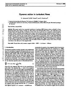
By OSCAR FLORES1. AND JAVIER JIM ´ENEZ1,2. 1School of Aeronautics .... Flack, Schultz & Shapiro (2005) report. Reynolds stresses, quadrant analysis and ...
c 2006 Cambridge University Press J. Fluid Mech. (2006), vol. 566, pp. 357–376. � doi:10.1017/S0022112006001534 Printed in the United Kingdom
357
Effect of wall-boundary disturbances on turbulent channel flows By O S C A R F L O R E S 1 1
AND
J A V I E R J I M E´ N E Z 1,2
School of Aeronautics, Universidad Polit´ecnica de Madrid, 28040 Madrid, Spain
2
Center for Turbulence Research, Stanford University, Stanford, CA 94305, USA
(Received 4 January 2006 and in revised form 11 April 2006)
The interaction between the wall and the core region of turbulent channels is studied using direct numerical simulations at friction Reynolds number Reτ ≈ 630. In these simulations the near-wall energy cycle is effectively removed, replacing the smooth-walled boundary conditions by prescribed velocity disturbances with non-zero Reynolds stress at the walls. The profiles of the first- and second-order moments of the velocity are similar to those over rough surfaces, and the effect of the boundary condition on the mean velocity profile is described using the equivalent sand roughness. Other effects of the disturbances on the flow are essentially limited to a layer near the wall whose height is proportional to a length scale defined in terms of the additional Reynolds stress. The spectra in this roughness sublayer are dominated by the wavenumber of the velocity disturbances and by its harmonics. The wall forcing extracts energy from the flow, while the normal equilibrium between turbulent energy production and dissipation is restored in the overlap region. It is shown that the structure and the dynamics of the turbulence outside the roughness sublayer remain virtually unchanged, regardless of the nature of the wall. The detached eddies of the core region only depend on the mean shear, which is not modified beyond the roughness sublayer by the wall disturbances. On the other hand, the large scales that are correlated across the whole channel scale with ULOG = uτ κ −1 log(Reτ ), both in smooth- and in rough-walled flows. This velocity scale can be interpreted as a measure of the velocity difference across the log layer, and it is used to modify the ´ scaling proposed and validated by del Alamo et al. (J. Fluid Mech., vol. 500, 2004, p. 135) for smooth-walled flows.
1. Introduction Wall-bounded turbulent flows have been thoroughly studied in the past decade, with special emphasis on flows over smooth walls. In the last few years increasing attention has been paid to the study of rough walls, which are commonly encountered not only in some industrial applications but also in the vast majority of geophysical flows. There are also theoretical aspects of rough-walled flows which might be useful for the understanding of the physics of the wall region, in particular its interaction with the outer flow. Direct numerical simulations (DNS) of non-physical flow configurations have been very useful in the study of inner-outer interactions, ´ such as in the autonomous channel of Jim´enez, del Alamo & Flores (2004). From this point of view, the study of rough-walled flows can be understood as the study of a core region without the structures of the smooth wall.
358
O. Flores and J. Jim´enez
From the experiments of Nikuradse (1933) it is known that the main effect of roughness is a decrease in the mean velocity profile, which is constant outside the immediate vicinity of the wall. This leads to the modified logarithmic law U + = κ −1 log y + + A+ − �U + = κ −1 log y/ks + 8.5,
(1.1)
where U is the mean streamwise velocity and y is the wall distance. Variables with a + superscript are expressed in wall units, using the friction velocity uτ and the viscous ´ an ´ constant is κ and A is the intercept constant, and they are length ν/uτ . The Karm usually taken as κ = 0.41 and A+ = 5.2 for smooth channels. The effect of the surface roughness on the mean velocity profile is accounted for by the roughness function �U + , or by the equivalent sand roughness ks+ , introduced by Schlichting (1936). This velocity decrease is generated in the wall region, and the mean velocity gradient remains unchanged in the logarithmic and outer regions. Also, due to the nature of the rough wall, there is an uncertainty in the position of the origin for y. Thom (1971) and Jackson (1981) show that a reasonable choice is the mean momentum absorption plane, obtained as the centroid of the drag profile on the roughness. Other methods for computing the origin of y, based on the assumption that there is a logarithmic layer in the mean velocity profile, are reported by Raupach, Antonia & Rajagopalan (1991). The classical theory is based on the ‘Townsend hypothesis’, that states that outside the roughness sublayer the turbulent motions at sufficiently high Reynolds number are independent of the wall roughness and of viscosity (Perry & Abell 1977; Raupach et al. 1991). This implies that, apart from the effect of the roughness on the mean velocity, no other differences between smooth- and rough-walled flows should be encountered. As reported in the recent review by Jim´enez (2004), this theory has been challenged during the past decade, and is still a subject of discussion. For instance, the experiments of Krogstad, Antonia & Browne (1992) in a boundary layer over a mesh-screen wall show important differences between the smooth- and the rough-walled cases in the outer region. The wall-normal velocity fluctuations are enhanced across the whole thickness of the boundary layer in the rough case, indicating that the active scales are modified everywhere. Krogstad & Antonia (1994) find that these modifications are associated with changes in the streamwise correlation length of all the velocity components, around half the size for the structures over rough walls that for those over smooth walls. In a later paper Krogstad & Antonia (1999) compare the mesh-screen and the smooth wall with a surface roughened with circular rods. This new rough surface also produces modifications in the turbulent structures of the outer region. In both cases, the differences in the velocity fluctuations are accompanied by differences in the Q2 and Q4 quadrant contributions to the Reynolds stresses, with increased sweep events in the rough-walled cases. A comparison of the spectra from the rough-walled cases with the smooth-walled ones shows differences for the v-spectrum and for the uv-cospectrum, while the u-spectrum compares well. Similar results are published by Djenidi, Elavarasan & Antonia (1999) for a d-type roughness on a boundary layer. They conclude that the effects of the surface condition are not confined to the inner region of the flow. The experiments of Poggi, Porporato & Ridolfi (2003) in turbulent channels indicate that the roughness decreases the levels of anisotropy and intermittency in the inner region. They suggest that the changes in the inner region modify the flow in such a way that the effects of the roughness are also present in the core region. Simulations in non-symmetric channels, with roughness
Wall disturbance effects on turbulent channel flows
359
elements only in one wall, also show important departures from the smooth-wall behaviour that extends to the centre of the channel (Leonardi et al. 2003; Bhaganagar & Kim 2003; Orlandi, Leonardi & Tuzi 2003), although it is unclear whether this is due to the roughness or to the asymmetry. On the other hand, other experiments over rough-walled boundary layers show excellent agreement with smooth-walled data in the outer region. Ligrani & Moffat (1986) show good collapse in the streamwise velocity fluctuations, although some anomalous scaling is reported in the other two velocity components. They also check that the smooth- and rough-walled streamwise spectra collapse in the overlap region, supporting the findings of Perry & Abell (1977) in pipes. Keirbulck et al. (2002) show velocity fluctuations profiles collapsing with smooth-walled data in the outer region, although the wall-normal velocity is affected by the roughness over up to 40% of the boundary layer thickness. The turbulent production and dissipation profiles are quite similar across the whole layer, while the wall-normal energy flux is very different for the rough and the smooth cases. Flack, Schultz & Shapiro (2005) report Reynolds stresses, quadrant analysis and velocity triple products collapsing with the smooth-walled data, within the experimental uncertainty, for rough-walled flows with δ � ks . A recent study in turbulent channels by Bakken et al. (2005), using their own experimental data and the DNS results of Ashrafian, Andersson & Manhart (2004), supports the idea that the wall roughness modifies the velocity fluctuation profiles only within the roughness sublayer, although some uncertainty exists about further effects within the outer region. The authors speculate that turbulent channel flows over rough walls satisfy the similarity hypothesis of Townsend but that the same may not be true for boundary layers. The present work aims to clarify how the outer turbulent flow is modified by the near-wall region, simulating the effect of the surface roughness with a distribution of velocities on the wall that replaces the non-slip and impermeability boundary conditions. The numerical setup and the boundary conditions are presented in § 2. The effect of this artificial roughness on the rest of the flow is discussed in § 3 using one-point statistics. The flow around the disturbances is characterized in § 4, and a spectral analysis of the effect of the roughness in the outer flow is conducted in § 5, emphasizing the effect of the wall disturbances on the largest scales of the outer region. Conclusions are offered in § 6. 2. Numerical experiment The present direct numerical simulation integrates the Navier–Stokes equations in the form of two evolution problems for the wall-normal vorticity ωy and the Laplacian of the wall-normal velocity ∇2 v. The time integration is performed using a third-order Runge–Kutta scheme with implicit viscous terms, as in Kim, Moin & Moser (1987). The spatial discretization is pseudospectral, with dealiased Fourier expansions for the streamwise (x) and spanwise (z) directions, and a compact finite differences scheme in the wall-normal direction (y). The periodicities of the computational box in the wall-parallel directions are Lx and Lz , while h is the half-height of the channel. We denote by u and w the streamwise and spanwise velocity fluctuations, and by W the mean spanwise velocity. The numerical scheme for the first derivative in the y-direction is a fourth-order spectral-like compact finite differences one (Lele 1992) based on a five-point stencil in a uniform mesh, which is analytically mapped to the actual stretched mesh of
360
O. Flores and J. Jim´enez
the simulation. The coefficients of the scheme are computed using two consistency conditions, and two extra conditions provided by the minimization of the L2 norm of the difference between the eigenvalues iα and i˜ α of the exact and discretized derivatives, in the range 0 < α�x < π. The resulting scheme has quite good resolution properties; the standard five-point eighth-order compact finite differences scheme resolves up to 61% of the numerical wavenumbers with less than 1% of error, while the modified scheme resolves up to 74% with the same accuracy. For the two points closest to the wall we use compact finite differences schemes with three-point stencils. A third-order scheme with a non-centred stencil is used for the point at the wall, and the next one uses a standard fourth-order centred scheme. It was found that improving the order of the scheme at the wall above the order of the scheme at the centre of the channel led to numerical instabilities, in agreement with the results of Kwok, Moser & Jim´enez (2001). These authors also show that boundary schemes one order lower than the interior scheme are adequate to ensure global convergence consistent with the order of the interior scheme. For reasons of numerical efficiency, the scheme for the second derivative, required to solve the Helmholtz equation for the viscous terms, is directly computed in the stretched mesh, and only the consistency conditions are used to compute the coefficients of the scheme. As for the first derivative, a five-point stencil is used, with non-centred stencils at the walls. The resulting scheme has sixth-order accuracy. The non-slip and impermeability boundary conditions for the velocity at the walls are replaced by prescribed zero-mean-value perturbation velocities. These velocities are characterized by the amplitudes and the streamwise and spanwise wavelengths (Λx and Λz ) of the single Fourier mode being forced. When only the wall-normal velocity component is disturbed, a fairly small effect on the flow is achieved, with �U + = 4.6 when the intensity of the wall-normal velocity disturbance is vw�+ = 0.72 (throughout this paper, the subindex w denotes variables evaluated at y = 0, the prime stands for root-mean-square averaging and �� stands for averaging both in time and in the two homogeneous directions). When the streamwise and the wall-normal velocities are forced with the same phase, so that the Reynolds stresses component �uv�w �= 0, �+ a much stronger effect on the flow is obtained. For instance, u�+ w = −vw = 0.83 + leads to �U = 8.7. Hence, two distinct forcings are used in this paper, both having �uv�w �= 0 and �uw�w = �vw�w = 0. The first one has u�w �= 0, vw� �= 0, ww� = 0 and will generally be represented in the figures with open symbols. The second forcing has u�w = vw� = ww� �= 0, and will be represented with solid symbols. In this case, w is shifted in x by Λx /2 with respect to u and v, so that the imposed velocity disturbances are non-symmetric and the flow just upstream of vw > 0 goes to the left, while the flow downstream goes to the right. These boundary conditions are quite different from those proposed by Orlandi et al. (2003), where an instantaneous velocity plane extracted from a full DNS simulation was used as boundary condition in one wall of the perturbed DNS. The advantages of the present approach are essentially the fuller control of the boundary condition and an easier parameterization of the artificial roughness. Both walls are forced in our case to obtain a symmetric configuration with a well-defined centre, where the turbulent structures can be compared with those of smooth channels. 3. One-point statistics The parameters of our numerical experiments are presented in table 1. Two different box sizes are used: simulation run numbers with upper-case letters denote big boxes,
361
Wall disturbance effects on turbulent channel flows
r1 r2 R2 r3 S0
Reτ Lx / h �x + �yc+ �yw+
u�+ w
vw�+
556 631 632 674 547
0.94 0.83 0.83 0.67 0
1.13 0.83 0.83 0.67 0
4π 4π 8π 4π 8π
10.2 11.6 11.6 12.4 13.4
7.0 8.0 8.0 8.6 6.7
0.8 0.9 0.9 1.0 1
(ωx� )+ Λ+ �U + w x 1.19 1.12 1.12 1.03 0.26
71 220 221 529
7.1 8.7 8.7 9.6
δy +
ks+
k+
−2.6 67 6.9 −11.2 128 15.5 −11.7 129 15.5 −20.7 207 24.4
h/k Λx /k 81 41 41 28
10.3 14.2 14.2 21.7
Table 1. Numerical simulation parameters. Reτ = uτ h/ν is the friction Reynolds number. Lx and Lz = Lx /2 are the streamwise and spanwise lengths of the computational box. The mesh resolution after dealiasing is �x, �z = �x/2. The wall-normal mesh resolution is �yc at the centre of the channel and �yw at the wall. u�w and vw� are the wall forcing intensities, (ωx� )w is the streamwise vorticity intensity at the wall, Λx and Λz = Λx /2 are the streamwise and spanwise wavelengths of the forcing. �U and δy are the velocity decrease and the wall-normal shift, obtained from a logarithmic law adjustment. ks is the equivalent sand roughness and k is a characteristic length of the forcing, defined in § 4.
Lx × Lz = 8πh × 4πh, and lower-case letters denote smaller ones, Lx × Lz = 4πh × 2πh. The cheaper small-box cases are performed to investigate the effects of different ´ forcings on the O(y) active scales of the outer flow. It is shown by del Alamo et al. (2004) that DNS with these box lengths are able to accurately represent most of the active scales of the turbulence, but do not contain the very large scales of the flow. Therefore, a large-box simulation R2 is used to study the effects of the mid-intensity forcing on these scales. The results from these four wall-disturbed simulations are compared with a DNS of a smooth-walled turbulent channel in a large box performed ´ by del Alamo & Jim´enez (2003), which is also included in table 1 as case S0. This numerical experiment has friction Reynolds number comparable to that of the forced cases. In the present simulations the method proposed by Thom (1971) to estimate the position of the wall is not applicable, and both the wall-normal shift δy + and the roughness function �U + are obtained by a least-square fit of the mean velocity profile to the logarithmic law (1.1) in the region between y + = 50 and y = 0.2h. The exact ´ an ´ constant used in the fitting produces variations in �U + , which value of the Karm are of about 15% when κ is varied in the range 0.38 − 0.42. The position of the wall also varies with κ, but in all cases δy + ≈ O(10). The values presented in table 1 are obtained for κ = 0.41. The equivalent sand roughness ks+ of the disturbed cases corresponds to the fully rough regime, except for r1 which may be classified as transitional. All the computed δy + are small compared with ks+ and with Reτ . A new wall-normal coordinate y¯ = y + δy (1 − y/ h)
(3.1)
is defined to expand the numerical wall-normal coordinate y from the interval [0, 2h] to [δy, 2h − δy]. It is interesting to note that δy is negative for all cases, which means that the effective wall (¯ y = 0) is above the plane in which the disturbances are injected into the flow (y = 0). In the smooth case S0 we have y¯ = y. The mean streamwise velocity profiles are presented in figure 1(a) expressed in wall units, and in velocity defect form in figure 1(b). Both figures are consistent with previous results obtained over rough walls in experiments (Bakken et al. 2005; Poggi et al. 2003) and in numerical simulations (Ashrafian et al. 2004; Leonardi et al. 2003; Orlandi et al. 2003). Only small deviations from the smooth-walled velocity defect ´ law are observed in figure 1(b). Similar differences were observed by del Alamo et al.
362
O. Flores and J. Jim´enez 20
0
(a)
–2 U +– Uc+
U+
15 10
–4
–6
5 0 100
(b)
–8 101
102 y¯ +
103
0
0.2
0.4
0.6
0.8
1.0
y¯ /h
Figure 1. (a) Mean streamwise velocity. (b) Streamwise velocity defect law, Uc = U (y = h). , S0; 䉭, r1; 䉮, r2; 䊊, R2; 䊏, r3.
(2004) when comparing smooth channels with different box sizes. They suggested that their discrepancies could be related to contributions from large scales to the mean flow, an argument that may also be valid for the present results. Although not obvious from the figure, ∂U/∂y at the wall in case r1 is roughly zero, which indicates that the mean flow above the disturbances is separated, with ∂U + /∂y + |w = −0.07 and min(U + ) = −0.01. This is due to the high value of vw� employed in this case. Similar locally separated flows are found by Jim´enez et al. (2001) in porous channels when the porosity coefficient exceeded a certain threshold. For the case r3 a secondary flow (not shown) is observed in the spanwise direction, with W (y) < 0.1U (y) everywhere, a maximum value of |W + | = 0.3 at y + = 40, and zero mass flux when integrated across the full height of the channel. The u� profile in the wall region is presented in figure 2(a). The intensity of the near-wall peak decreases as the roughness function increases, and the same is true for the off-wall peak of the streamwise vorticity intensity ωx� in figure 2(b). In both cases, the attenuation of the peak is due to the shortening of the spectra, which will be discussed in § 5. The maximum value of ωx�+ is always at y = 0. In the smooth case this is due to the interaction of the wall with the transverse velocities created by the quasi-streamwise vortices (Kim et al. 1987). In the disturbed cases, that component is probably also present, but a much larger contribution comes from the forcing itself (see table 1). The off-wall peaks of u� and ωx� are indicators for the near-wall streaks and for the quasi-streamwise vortices. In smooth channels those structures are involved in the self-sustaining near-wall energy cycle described by Jim´enez & Pinelli (1999), which is responsible at the present Reτ for roughly 35% of the total energy production in the channel. The damping of those peaks in figures 2(a) and 2(b) suggests that the cycle is perturbed in case r1, strongly perturbed in r2 and R2, and essentially destroyed in r3. Those changes are also reflected in the ratio of the production (Π) to the dissipation (ε), shown in figure 2(c). In the smooth-walled case there is a production peak at y¯+ ∼ 20, and a slightly dissipative layer in 40 < y¯+ < 100. As the roughness function increases, this peak decreases and the dissipative region disappears. There is a new peak of Π/ε just above the wall which is due to the additional Reynolds stress introduced by the forcing, and which has been highlighted in the figure with a dashed line. In the case R2 both peaks form the two ends of a plateau, but for r3 the new peak dominates and the old one has essentially disappeared. In all cases the
363
Wall disturbance effects on turbulent channel flows 3.0 2.5
0.25
2.0
0.20
u′ + 1.5
ωx′ + 0.15
1.0
0.10
0.5
0.05 (a)
0 –20
0
20
40
60
80
(b) 0 –20
100
0
20
40
60
80
100
1.0
1.8 1.6
0.5 1.4
Π ε 1.2
Φ+
0
1.0 –0.5
0.8 (c)
0.6 –20
0
20
40 y+
60
80
(d) 100
–1.0 –20
0
20
40 y+
60
80
100
Figure 2. Near-wall behaviour. (a) Intensities of the streamwise velocity fluctuations and (b) of the streamwise vorticity. (c) Ratio of turbulent energy production to dissipation. , S0; 䉭, r1; 䉮, r2; 䊊, R2; 䊏, r3. (d) Turbulent energy flux, defined in (3.2).
dissipation at the wall is much larger than the production, and the wall acts a net energy sink. Figure 2(d) presents the energy flux Φ, computed by evaluating each term of Φ=
1� 2 � ν ∂ 2 � 2� ui v + �vp� − u , 2 2 ∂y 2 i
(3.2)
where the subindex implies a summation for all the velocity components, and p is the pressure fluctuation. In smooth-walled flows, part of the energy produced around y¯+ ∼ 20 is exported towards the centre of the channel (Φ > 0), to be dissipated by the background turbulence, while the rest is exported towards the wall (Φ < 0), where it is absorbed by the viscosity. The maximum of Φ near y¯+ = 40 is compensated by the extra dissipation shown in figure 2(c) at that level. For the disturbed cases, the energy also flows both towards the centre and towards the wall, but the maximum at y¯+ = 40 progressively disappears, together with the dissipative layer. The energy structure in the near-wall layer looks very different in the smooth and in the disturbed cases, and it is clear that in the latter the canonical cycle of the smooth-walled channel has been severely perturbed. It is therefore significant that far from the wall all the variables tend to their smooth values. The comparison is extended to the whole channel in figure 3. Except near the wall all the cases agree. Specially significant is the energy flux. There is in all cases a region where Π/ε ≈ 1, which suggests the formation of an equilibrium overlap layer. That is a local property of the turbulence at that wall distance, consistent with the usual arguments for a logarithmic law. Those arguments only require that Φ should be constant across that
364
O. Flores and J. Jim´enez 2.5
1.5
2.0 u′ +
1.5
w′+ v′+
1.0
w′+
1.0 v′+ 0.5
0.5 (a) 0
0.2
0.4
0.6
0.8
(b) 0
1.0
0.2
0.4
0.6
0.8
1.0
(c) 0.4
1.5
0.2 Π 1.0 ε
Φ+
0 –0.2
0.5
–0.4 –0.6
(d)
–0.8 0
0.2
0.4
y–/h
0.6
0.8
1.0
0
0.2
0.4
0.6
0.8
1.0
y–/h
Figure 3. Turbulent statistics in the outer region. (a) Intensity of the streamwise velocity fluctuations and (b) of the wall-normal and spanwise velocity fluctuations. (c) Ratio of , turbulent energy production to dissipation. (d) Turbulent energy flux, defined in (3.2). S0; 䉭, r1; 䉮, r2; 䊊, R2; 䊏, r3.
region, but they say nothing about its actual value. In order to investigate whether this value is fixed by the wall, by the outer region or by the log layer itself, we can compare Φ for flows with different wall regions (smooth and rough walls) and for flows with different outer regions (channels and boundary layers). As Φ is not always available in experiments, we will also use �u2 v�, which in (3.2) accounts for roughly one half of Φ. The collapse shown in figure 3(d) and the results reported by Bakken et al. (2005) in channels and Flack et al. (2005) in boundary layers suggest that the energy flux in the overlap region is not imposed by the wall. On the other hand, Jim´enez & Simens (2000) report that �u2 v�+ collapses in the overlap region for turbulent channels and for boundary layers. This evidence suggests that the level of Φ + ≈ 0.3 should be intrinsic to the log layer, instead of dependent on its boundary conditions. It is also interesting in figure 3(b) that the transverse intensities v � and w� increase near the wall as the roughness increases, even as ωx� decreases. Examination of their spectra shows that the extra energy is essentially isotropic in the wall-parallel plane, and therefore unrelated to the usual vortices found over smooth walls. The collapse of the velocity fluctuation intensities, of the ratio of the production to the dissipation, and of the energy flux in the outer region agrees with most of the literature comparing flows over smooth and rough walls, as already mentioned in the introduction. It however disagrees with Krogstad et al. (1992), where the high growth rate of the boundary layer thickness may introduce distortions in the wall-normal mean velocity component. Orlandi et al. (2003) also find a different behaviour in channels with only one rough wall, but their mean profiles are asymmetric, and the
365
Wall disturbance effects on turbulent channel flows 5
0 (a)
4 3 ∆c+ω
–0.5
2 –1.0
1 0
–1.5
–1 –2
(b) 0
50
100 y– +
150
200
0
0.2
0.4
0.6
0.8
1.0
y–/h
Figure 4. Advection velocities in the outer region. �cω+ computed for all wavenumbers, , plotted as a function of the wall distance (a) in wall units and (b) normalized with h. S0; 䉭, r1; 䊊, R2; 䊏, r3.
additional shear introduced by the difference in wall friction between the smooth and the rough wall is not negligible at moderate Reynolds numbers. That extra shear may modify the structures in the core region of the channel, as reported in asymmetric channels by Hanjali´c & Launder (1972). As expected, the results from cases r2 and R2 are almost indistinguishable in figures 2 and 3, and only R2 will be used from now on. The good agreement between the two boxes confirms that the 4πh × 2πh boxes contain most of the active scales in the turbulent channel flow. We can also analyse the effect of the wall on the advection velocity of the u structures, which corresponds to that of ωy in the limit of elongated structures. The method used here to compute the advection velocity was previously used by Jim´enez et al. (2004), and is based on the equation satisfied by a simple wave, �) c, �) = −kx (� ϕ∗ · ϕ Im(� ϕ ∗ · ∂t ϕ
(3.3)
� is the corresponding Fourier mode, kx is the streamwise where c is the phase velocity, ϕ wavenumber and the asterisk indicates complex conjugation. This equation only holds for a single Fourier mode. For larger sets of wavenumbers it can be generalized by averaging the spectral quantities on both sides of (3.3), so that the advection velocity of ωy is defined as � y �Ω Im�� ωy∗ · ∂t ω cω = − = U + �cω , (3.4) ∗ � y �Ω �y · ω �kx ω where ��Ω implies that the average is taken over all the wavenumbers in the Fourier domain Ω. Note that the term �cω contains the nonlinear advection and viscous contributions, but not the mean velocity U . Therefore, �cω describes the interaction of ωy with the mean flow, and is a first-order indicator of the dynamics. A comparison of (3.4) with the more usual definition of advection velocity given by ´ Wills (1964) is documented in del Alamo et al. (2006a). On the other hand, since the same definition is used here for both the rough- and the smooth-walled simulations, the exact relationship of cω with the advection velocity of Wills (1964) is not critical for the purposes of this section. Figure 4 presents the distribution of �cω+ with respect to the wall distance, computed over the whole wavenumber domain. Figure 4(a) shows that near the wall the distribution of �cω+ is very different in the four cases. The smooth-walled channel has
366
O. Flores and J. Jim´enez
higher �cω+ at the wall than the disturbed cases, due to its higher ∂U/∂y|w , and also because of the negative contribution to �cω+ of all the structures which are essentially attached to the wall forcing. The negative peak in S0 around y¯+ ≈ 30 is damped in R2 and r3, as a consequence of the interruption of the near-wall cycle in the latter. In the transitional case r1 this peak remains roughly unchanged, and the more intense negative peak below it is again due to the structures attached to the wall forcing. Despite the big differences observed near the wall, the disturbed cases tend to the smooth-walled values as y¯+ increases, and figure 4(b) shows that they compare well for y¯ > 0.2h. This suggests that to a first approximation the dynamics of the outer region is not modified by the wall. This result is consistent with the advection velocities of u computed by Sabot, Saleh & Comte-Bellot (1977) in rough- and smooth-walled pipes, using space-time correlations for the large-streamwise-separation limit. 4. Box-filtered flow fields In § 3 we have seen that the present forcing is able to strongly modify the near-wall region of a smooth-walled channel, essentially destroying its energy cycle. In fact, the flow just above the wall is very complex, with locally separated regions (u < 0) attached to the areas being blown (vw > 0), and high velocity gradients over the regions under suction (vw < 0). Because of that inhomogeneity, plane-averaged quantities are not adequate to study the flow features near the wall, while the instantaneous realizations are always hard to interpret. Hence, we compute the averaged flow in boxes of size Λx × Λz /2 × h containing a forcing cell, which consists of a single blowing and a single suction. This box averaging is performed using a Fourier filter that retains only those modes which are conserved by the group of translations in physical space that keeps the forcing invariant, but excluding the uniform (0, 0) mode. Note that strict time averaging of the velocity fluctuations, without the homogeneity assumption, would lead us to a flow field composed of these averaged boxes. This is true provided that the forcing does not develop subharmonical perturbations before breaking in fully developed turbulence, which is confirmed by the spectral analysis. We denote with the subindex B the variables averaged in this way. They only contain the fluctuations that are associated with fixed positions relative to the wall forcing. It is possible to derive an equation from them, by time averaging the Navier– Stokes equations for the velocity fluctuations. In the resulting equations, and for wall distances y ∼ Λx where U � uτ & uB , the advection by the mean velocity and the pressure term are dominant, while the advection due to uB and the Reynolds stresses produced by the remaining velocity fluctuations are negligible. This leads to the linearized Rayleigh equation, whose solution for y ∼ Λx decays as � √ (4.1) uB ∼ exp(− Kx2 + Kz2 y) = exp(−2π 5y/Λx ), where Kx = 2π/Λx and Kz = 2π/Λz are the wavenumbers of the forcing. Note that, in the present simulations with Λx = 2Λz , there is no difference in using Λx or (Kx2 + Kz2 )−1/2 , except for a constant factor. Figure 5(a) shows (uB )�+ as a function of the wall distance normalized with the wavelength Λx of the forcing. Near the wall, (uB )�+ accounts for most of u� , but it tends to zero as y increases. The ground level of (uB )�+ ≈ 10−3 for y > 0.6Λx is consistent with the expected uncertainty due to the limited number of forcing cells used for the statistics, which is 5 × 10⁴ − 5 × 10⁵ for the 150 available fields. Nevertheless, the statistics are good enough to observe the predicted exponential decay.
367
Wall disturbance effects on turbulent channel flows (a)
10–1
(b)
100 10–1 uF′ +
(uB)′+, uF′+
100
10–2
10–2
10–3
10–3 0
0.2
0.4
0.6
0.8
1.0
y/Λx
0
5
10 y/k
15
20
Figure 5. Streamwise velocity fluctuations near the wall, (uB )�+ from box-averaged flow fields (lines), and u�+ F from filtered spectra (symbols). (a) Wall distances normalized with Λx . 䉭, and , r1; 䊊, and , R2; 䊏, and , r3. The dotted straight line is (4.1). (b) Wall , S0 using the filter and distances normalized with k, defined in (4.2). 䉭, r1; 䊊, R2; 䊏, r3; the value of k calculated for r1; the dashed vertical line is y¯ = 6k.
Similar exponential decays are also observed for the other two velocities and for all the components of the vorticity vector. However, the tangential Reynolds stress �uB vB � of the rough cases does not collapse either with y + or with y/Λx or with y/ h. Hence, we define a new length scale � h (4.2) k = − �uB vB �+ dy, 0
that corresponds to the height at which the full tangential Reynolds stress u2τ would exert the same moment as the actual �uB vB � distribution. This definition is similar to the method proposed by Jackson (1981) to calculate the origin for y, defined as the position at which a uniform stress would exert the same moment on the flow as the real rough wall. It is interesting that in the present cases k is roughly equal to the maximum height of the separated flow regions of the box-averaged fields (uB < 0), located above the areas being blown. The wavelength Λx and k are not proportional, as can be observed in the last column of table 1. In fact, k is not only dependent on Λx , but also on the other parameters of the forcing and on the Reynolds number of the flow. However, if we assume that (4.1) applies for the whole wall region with (uB )�w = −(vB )�w = uτ , and that uB and vB are in phase, we can integrate (4.2) to get √ Λx ≈ 2π 5. (4.3) k This crude estimate of k gives values which are of the same order as those in table 1. Figure 5(a) also shows u�+ F , which is the square root of the sum of the filtered spectra, where the filter is the one defined at the beginning of the section. Note that u�F 2 contains both (uB )�2 and the incoherent contribution of the velocity in the forced modes. Therefore, u�F agrees with (uB )� near the wall, and decays with y/Λx until the slope of u�+ F changes. The wall distance at which the change occurs does not scale with Λx , as can be observed in the symbols of figure 5(a). On the other hand, when u�+ F is plotted as a function of y/k in figure 5(b), the change in the slope takes place at about y ∼ 6k for the three rough cases. In the layer below 6k, limited by the dashed line in the figure, the non-homogeneous contribution from the forcing dominates the background-filtered turbulence, and thus it can be interpreted as the roughness sublayer associated with the disturbed boundary condition. For reference,
368
O. Flores and J. Jim´enez 100 (b)
(a)
y h
λz 0 h 10
10–1
100
λx /h
101
100
λx /h
101
Figure 6. Premultiplied spectra of the streamwise velocity, normalized with u2τ . (a) At a fixed wall distance y¯ = 0.5h. The contours are 1/3 and 2/3 of the maximum of S0. (b) Wall-normal distribution of the spectra, summed for all spanwise wavelengths and premultiplied by the streamwise wavenumber. The contours are 1/8, 1/4 and 1/2 of the maximum of the smooth , S0; 䉭, r1; 䊊, R2; 䊏, r3. case.
figure 5(b) also includes the energy contained in case S0 computed with the filter from case r1. The wall-normal distance is also normalized with the value of k obtained for r1. The collapse of u�+ F from r1 and S0 supports that turbulence is not affected by the boundary condition outside the roughness sublayer. This roughness sublayer substitutes the buffer region of smooth walls, and it is between it and the outer region where the overlap region is located, 6k < y < 0.2h. In this region the tangential Reynolds stress is almost constant, and we can apply the same arguments used for the logarithmic region of smooth-walled flows. 5. Spectral analysis More details about the influence of the disturbances in the channel flow can be extracted from spectral analysis. Figure 6(a) shows the premultiplied spectrum of the streamwise velocity fluctuations in the core region for the disturbed and for the smooth-walled cases, at y¯/ h = 0.5. The collapse is excellent, except for the longest wavelengths, supporting the hypothesis that the effect of the wall disturbances is confined to the roughness sublayer. Even better collapse is found for the other two velocity components, in which the large-scale modes do not contain energy. The minor differences found in the smallest scales are due to the differences in the Reynolds numbers, as this region of the spectrum collapses when the wavelengths are expressed in wall units. When we check the wall-normal distribution of the streamwise spectrum of u (figure 6b), we observe that the situation presented in figure 6(a) holds for most of the channel, with good agreement between the smooth and the rough cases for y¯/ h ≈ 0.2–1. As expected, strong differences are observed at wall distances corresponding to the buffer region over smooth walls, with the streaks becoming shorter and eventually disappearing as the roughness function increases, in agreement with the results presented in figure 2. In the disturbed cases, the narrow peaks located at λx < h contain around 13% of the energy in the roughness sublayer, and correspond to the wavenumber of the forcing and to its harmonics. The total energy contained in these modes is u�2 F , discussed in § 4. The other two velocity components and the uv-cospectrum (not shown) for the rough cases also agree with the smooth
369
Wall disturbance effects on turbulent channel flows 1.0
1.0
(a)
y h
(b)
0.8
0.8
0.6
0.6
0.4
0.4
0.2
0.2
0
–3
–2
–1
0 ∆x/h
1
2
3
0
–0.4
–0.2
0 0.2 ∆x/h
0.4
0.6
Figure 7. Correlation coefficients for zero spanwise separation. (a) ρuu , (b) ρvv . The contours , S0; , R2. correspond to 0.1, 0.2, 0.3, 0.6, 0.9.
channel in the outer region. The spectra presented in figure 6 are consistent with the agreement in the outer region between the smooth- and rough-walled velocity fluctuation intensities presented in figure 3. These results contradict those reported by Krogstad et al. (1992), Krogstad & Antonia (1994) and Krogstad & Antonia (1999) in boundary layers. In their experiments, the roughness strongly affects the wall-normal velocity through the whole layer, and the correlation lengths in the streamwise direction for u and v are twice as long for the smooth-walled case as for the rough-walled one at all heights. Note that, although the spectrum is the Fourier transform of the correlation, separation and wavelengths have different meanings, and it is not possible to directly compare spectra and correlations. Therefore, to check for the change in the correlation lengths in the present simulations, figure 7 shows the correlation coefficients ρuu and ρvv , which are defined as ρrs (�x, �z, y¯, y¯0 ) =
�r(x, y¯, z, t)s(x + �x, y¯0 , z + �z, t)� . r � (¯ y )s � (¯ y0)
(5.1)
In the above equation �x, �z are the separations in the homogeneous directions, y¯, y¯0 are the wall distances and r, s are the corresponding velocity components. The reference wall distance used in the figure is y¯0 = 0.16h, as in Krogstad & Antonia (1994). There are large differences in the wall region between S0 and R2, both in ρuu and in ρvv , located upstream from the reference location and at wall distances and streamwise separations that roughly correspond with the near-wall streaks. There are also smaller differences for y¯ > 0.2h, which are clearer for the largest separations of ρuu . However, these differences do not account for the large changes in the correlation length documented by Krogstad & Antonia (1994), except in the wall region. When the same plots are drawn for y¯0 = 0.5h (not shown), the contours of the correlation coefficients for S0 and R2 coincide better, although some differences are still observed for the longest separations. In figure 7(b) we can observe that the blocking effect of the smooth wall on v is relaxed for the rough-walled case, and the contours of ρvv in R2 are closer to the wall than those in S0.
370
O. Flores and J. Jim´enez 101 (a)
0.35
(b)
0.30 0.25 λz h
100
q+
0.20 0.15 0.10
10–1
100
0.05
101
0
λx /h
0. 4
0.6
0.8
1.0
y/h
1
1.0
(c)
(d)
0.8 y h
0.2
0.8
0.6
0.6 F
0.4
0.4
0.2
0.2
0
100
λx /h
101
0
0.2
0.4
y/h
0.6
0.8
1.0
Figure 8. (a) Correlation height Huu , as defined in (5.2). The contours correspond to 1/2 and 3/4, increasing from left to right. The grey patch corresponds to 1/3 of the maximum of the premultiplied streamwise velocity spectra of case S0, at y¯ = 0.5h. (b) Energy contained in the global modes, 6h < λx < 24h and λz > h. (c) �cω+ computed for λz > h, see (3.4). The contours, , S0; 䉭, r1; 䊊, R2; 䊏, r3. from top to bottom correspond to �cω+ = −1, 0, 1. In (a–c) + . (d) Structure function F , defined in (5.3), computed for 6h < λx < 24h In (b), × is 1.15 qR2 ´ , Reτ ≈ 2000 (Hoyas & Jim´enez 2006); , Reτ ≈ 950 (del Alamo et al. and λz > h. , Reτ ≈ 550 (S0); 䊊, Reτ ≈ 630 (R2). 2004);
5.1. Global modes The differences observed in figure 7(a) between S0 and R2 in the outer region for long separations are consistent with those observed in the streamwise velocity spectrum. Note that in figure 6(a) there is an energy peak for S0 for λx > 10h at λz ∼ 2h, which is not visible in R2, suggesting that the very long scales are affected by the wall disturbances. In fact, very large structures in turbulent channels are known to be correlated from the wall up to the centre of the channel, as shown by Bullock, ´ Cooper & Abernathy (1978) and by del Alamo & Jim´enez (2003), and it is not surprising that they are modified everywhere in response to changes at the wall. These global modes are also present in the disturbed cases. This is demonstrated in figure 8(a), where the correlation height Huu of the streamwise velocity, � h� h 2 (λx , λz ) = Cuu (λx , λz , y, y0 ) dy dy0 , (5.2) Huu 0
0
is plotted as a function of the streamwise and spanwise wavelengths. The correlation coefficient Cuu between individual Fourier modes is the modulus of the Fourier transform of the spatial correlation ρuu defined in (5.1). The four cases agree well in
Wall disturbance effects on turbulent channel flows
371
figure 8(a), in particular the two large boxes S0 and R2. The global modes, defined as those for which Huu > 0.75h, are roughly located in λx > 6h and λz > h. In figure 8(b) we have represented the energies qS0 and qR2 contained in the modes with streamwise wavelengths in the range 6h < λx < 24h and spanwise wavelengths in the range λz > h. We do not include the energy of the two longest wavelengths of the simulation to avoid effects coming from the long-wavelength truncation of the spectra. For the same reason, only the cases in the long boxes R2 and S0 are considered. In the figure, the energies normalized with u2τ do not collapse, and the + small peak at y¯ ≈ 0.05h in qS0 , which is related to contributions from the streaks to + . However, for y¯ > 0.1h the shape of the global the global modes, is not present in qR2 modes intensities is the same for S0 and R2, and their differences can be accounted + + by a constant factor, qS0 ≈ 1.15qR2 , as can be observed in the extra line of figure 8(b). + + and qR2 are not observed in the The reason why the differences between qS0 streamwise velocity fluctuations presented in figure 3(a) is because their effect is weak for the present Reτ . The fraction of the total energy at each wall distance carried by the global modes is less than 25% for the present Reynolds numbers. Therefore, the difference shown in figure 8 corresponds to less than 4% of the total energy. Figure 8(c) shows the λx –y distribution of the advection velocities �cω+ defined in (3.4), averaged over those modes with λz > h. They compare well, especially for the two cases computed on large boxes, suggesting that the dynamics of the global modes are essentially the same over smooth and rough walls. In figure 8(d) we see another indicator that the differences in the structure of the global modes are a matter of intensity. This figure shows the structure function F =�
ˆ v ∗ �Ω −Re�uˆ , �uˆ uˆ ∗ �Ω �ˆv vˆ ∗ �Ω
(5.3)
where the Fourier domain Ω is 6h < λx < 24h and λz > h. Only data from long computational boxes are included in the figure, as well as two extra numerical ´ et al. experiments of turbulent channels with smooth walls at Reτ = 950 (del Alamo 2004) and Reτ = 2000 (Hoyas & Jim´enez 2006). The disturbed and the smooth-walled cases compare well, especially for S0 and R2 outside the wall region. Any variations seem to be connected with the Reynolds numbers of the different smooth-walled cases. The collapse again supports the idea that the wall does not modify the structure and the dynamics of the global modes. The high value of F for most of the channel implies that u and v are strongly correlated for long streamwise wavelengths, and therefore the global modes are very efficient in ´ generating Reynolds stresses (del Alamo & Jim´enez 2001). ´ According to del Alamo et al. (2004), the proper scale for the energy in the global modes in turbulent flows over smooth walls is Uc2 , because they are created by stirring the mean velocity profile all across the channel height. However, figure 8(b) shows that this scaling fails for our disturbed case, because the ratio of the energy in the global modes of S0 and R2 is much smaller than the actual ratio of their centreline velocities. The same happens with the mixed scaling (uτ Uc ) of DeGraaff & Eaton (2000). At this point there are two possibilities: either the velocity scale of the global modes depends on the roughness or it does not. Unfortunately, we do not have enough data to analyse this question directly. However, the scaling of the global modes is also eventually felt in the intensity of the streamwise velocity fluctuations as the Reynolds number increases, and there are more experimental intensities than spectral data
372
O. Flores and J. Jim´enez 4.5 10
U*+– Uc+
3.5
2
(u′+) y = 0.3h
4.0
3.0
5
0 2.5 (a)
(b)
2.0 200
400
600 (Uc+)2
800
–5 100
1000
2
101
10
103
ks+
4.5
3.5
2
(u′+) y = 0.3h
4.0
3.0 2.5 (c) 2.0
200
300
400
500
600
700
+ (U LOG )2
Figure 9. (a) Streamwise velocity fluctuations at y¯ = 0.3h as a function of (Uc+ )2 . (b) Difference between Uc+ and the ad hoc velocity scale U∗+ for rough-walled flows. (c) Streamwise velocity + fluctuations at y¯ = 0.3h as a function of (ULOG )2 . Open symbols denote rough-walled flows, and closed symbols denote smooth-walled flows. 䊊, channels from Ashrafian et al. (2004), Bakken et al. (2005) and Comte-Bellot (1965); 䉭, pipes from Perry & Abell (1977) and Perry ´ et al. (1986); ×, superpipe from Morrison et al. (2004); 䉮, present channels, del Alamo et al. , is (5.5). In (b), , (5.6). In (c), , (2004) and Hoyas & Jim´enez (2006). In (a), + )2 and , (u�+ )2 = 2.5 + 2 × 10⁻² (U + (0.2h) − U + (50ν/uτ ))2 . (u�+ )2 = 1.2 + 5.5 × 10⁻³ (ULOG
in the literature. Note that rough-walled flows are very sensitive indicators for any anomalous scaling of the fluctuations, because the range of Uc is larger than in smooth-walled flows. We will limit ourself to turbulent flows in channels and pipes, as the structure of the outer region for external flows might be different. ´ Following del Alamo et al. (2004), the intensity of the streamwise velocity fluctuations when y¯/ h & 0.2 should have the form y )u2τ + f (¯ y / h)U02 . u�2 ∼ log2 (h/¯
(5.4)
It has two components: one coming from the active eddies, proportional to u2τ , and another one proportional to the square of the characteristic velocity of the global ´ et al. (2004) is that U0 = Uc , a possibility modes, U0 . The proposal of del Alamo that is explored in figure 9(a), where we have plotted (u�+ )2 at a given wall distance y¯/ h = 0.3 for several pipes and channels. We can see a relatively good collapse of the smooth-walled data along the dashed line corresponding to the linear law (u�+ )2 = 0.94 + 3.7 × 10⁻³ (Uc+ )2 ,
(5.5)
Wall disturbance effects on turbulent channel flows
373
which is a particular case of (5.4) with U0 = Uc , except for the single unexplained data set from Morrison et al. (2004). As expected, the different rough-walled cases do not collapse with the same law, and their streamwise velocity fluctuation intensities are generally higher than those expected from their centreline velocities. We therefore work backwards and define U∗ as the velocity scale that collapses each rough-walled data point of figure 9(a) onto (5.5), and plot in figure 9(b) the values of U∗+ − Uc+ as a function of the equivalent sand roughness. The data collapse around the line U∗+ − Uc+ = κ −1 log(ks+ ) + A+ − 8.5 = �U + .
(5.6)
−1
This suggests that ULOG = uτ κ log(Reτ ), which can be interpreted as a measure of the velocity jump across the logarithmic layer, might be a better velocity scale for the global modes than Uc . We test this scaling in figure 9(c), where we can observe that the rough- and smooth-walled data now compare much better. Note that while U∗ is computed ad hoc for each data point of figure 9(a), ULOG is computed a priori for figure 9(c). Similar results are obtained for other wall distances in the range y¯/ h > 0.2. + is constant to a first-order approximation, Since for smooth-walled flows Uc+ − ULOG using U0 = ULOG instead of U0 = Uc only introduces a small square-root correction ´ to the law given by del Alamo et al. (2004). This correction is not observable when comparing the collapse of smooth-walled data over the limited range of Uc in figures 9(a) and 9(c). Note that, depending on the two limits assumed for the logarithmic layer, we could have added a constant to our definition of ULOG . Unfortunately, the scatter of the data is too high to distinguish between reasonable values for that constant. For example, the solid line in figure 9(c) corresponds to the least-square fit of the data to the velocity jump between y + = 50 and y/ h = 0.2, according to our definition of the log layer given in § 3. It can be observed in the figure that, for the available range of Reynolds numbers, this fit works as well as ULOG . Accurate measurements at higher Reynolds numbers are needed to evaluate that constant. ´ A similar conclusion was reached in del Alamo et al. (2004), where it was found that to distinguish between two different scales Reτ would have to be higher than 108 . Note on the other hand, that the collapse with ULOG as opposed to Uc is unambiguous, because there are big differences between both quantities for rough and smooth walls. All that can be said is that u� does not scale exclusively on uτ , and figures 9(a) and 9(c) give strong evidence that the other velocity scale is much closer to ULOG than to Uc .
6. Conclusions We have studied the effect of the boundary condition at the wall on the outer region of turbulent channel flows. The non-slip and impermeability boundary conditions that are natural to smooth walls have been replaced by a single-harmonic velocity disturbance with non-zero tangential Reynolds stresses at the wall. Three different forcings have been explored, in order to understand the effect of the different parameters characterizing the perturbations. We have shown that the main effect of the wall disturbances on the flow is the modification of the mean streamwise velocity gradient in the wall region, resulting in a constant velocity decrease across the whole channel. Also, the wall region in the disturbed channels is completely different to that over smooth walls. The streaks and the quasi-streamwise vortices are shortened, and consequently the intensities of
374
O. Flores and J. Jim´enez
the streamwise velocity fluctuations and of the streamwise vorticity decrease. On the other hand, the wall-normal and spanwise velocity fluctuations are enhanced by the disturbances. This increase is related to structures which are essentially isotropic in the wall-parallel plane, and which add little to the streamwise vorticity intensity. All of those are consequences of the disruption of the near-wall energy cycle by the disturbances at the wall, as is indicated by the reduction of the peak of energy flux from the walls towards the centre of the channel in the disturbed cases. The ratio of production to dissipation and the energy flux shows not only that the disturbances interrupt the near-wall energy cycle, but also that the introduced Reynolds stress generates additional energy that is mostly absorbed by the wall. Since some of those changes are typically encountered in turbulent flows over rough walls, we have interpreted the present boundary condition as a method for simulating the effect of the roughness without having to deal with the details of the flow around the roughness elements, as previously suggested by Jim´enez (2004). Hence, we have characterized the different wall forcings by their equivalent sand roughness. Three of the cases correspond to the fully rough regime, while the remaining one is transitional. We have analysed the flow over individual forcing cells by computing the averaged flow field around a single disturbance. The characteristic length scale for the decaying of the velocity disturbances is the forcing wavelength, but the tangential Reynolds stress has its own characteristic length scale, k. The height of the layer where the intensity of the forcing and its harmonics overrides the background turbulence is roughly 6k. This layer can be interpreted as a roughness sublayer, which in rough-walled flows plays the same role as the buffer layer over smooth walls. Special attention has been paid to the effect of our wall disturbances on the outer flow. Using one-point statistics we have shown that the smooth-wall values are recovered in the disturbed cases when y¯+ increases, and across the whole outer region. The spectral analysis and the advection velocities have shown that the structure and the dynamics of the detached scales of the core region in the present simulations are not affected by the perturbations imposed at the walls. This conclusion is coherent with the idea that the detached eddies are controlled by the local mean shear, which is only modified within the roughness sublayer. This is also consistent with the physical ´ model proposed by del Alamo et al. (2006b) for the logarithmic region, with a cluster of vortices developing a low-velocity wake due to the effect of the mean shear. While in the smooth-walled case the process is triggered by the bursting of the near-wall cycle, over rough walls it might be triggered by the disturbances at the wall. The fact that the same result is obtained for three different forcings, with very different wavelengths and intensities, even when the near-wall energy cycle of smooth walls is effectively destroyed, strongly supports the insensitiveness of the detached scales to the boundary condition, and its extension to real rough-walled flows. We have also seen that the dynamics of the larger scales of the flow are essentially the same over the forced and smooth walls They are global modes, in the sense that ´ they are correlated across the whole channel. In smooth-walled flows, del Alamo et al. (2004) showed that they scale with the centreline velocity Uc , and that therefore the square of the velocity fluctuations increase with Uc2 for a given wall distance. We have shown that this scaling does not work for rough-walled flows, and we have proposed a new velocity scale ULOG = uτ κ −1 log(Reτ ) for the global modes. As shown in figure 9(c), the modified scaling collapses the streamwise velocity fluctuations regardless of the nature of the wall. ULOG can be interpreted as a measure of the velocity difference across the logarithmic layer.
Wall disturbance effects on turbulent channel flows
375
The present work suggests that the outer flow region is fairly independent of the ´ wall layer, even if the opposite is not true (del Alamo & Jim´enez 2003; Hoyas & Jim´enez 2006). Even in rough-walled boundary layers it could be expected that the detached eddies remain unchanged, at least if the mean shear does. On the other hand, the effect of the roughness on the largest scales of boundary layers and of channels might be different. While the effect of the roughness on the global modes is symmetric in channels, in boundary layers only the wall is modified, and the free stream remains unchanged. Finally, higher Reynolds numbers are needed to analyse the effect of the wall on the overlap region, although some of the results presented in this paper, such as the constant energy flux discussed in § 3, suggest that the effect of the wall is also weak in that region. This work was supported in part by the Spanish CICYT, under grant DPI200303434. The computational resources provided by the CIEMAT in Madrid, by the CEPBA and by the BSC in Barcelona are gratefully acknowledged.
REFERENCES ´ del Alamo, J. C., Flores, O., Jime´ nez, J., Zandonade, P. & Moser, R. D. 2006a The linear dynamics of the turbulent logarithmic region. In preparation. ´ del Alamo, J. C. & Jime´ nez, J. 2001 Direct numerical simulation of the very large anisotropic scales in a turbulent channel. In Annu. Res. Briefs, pp. 329–341. Center for Turbulence Research, Stanford University. ´ del Alamo, J. C. & Jime´ nez, J. 2003 Spectra of the very large anisotropic scales in turbulent channels. Phys. Fluids 15, L41–L44. ´ del Alamo, J. C., Jime´ nez, J., Zandonade, P. & Moser, R. D. 2004 Scaling of the energy spectra of turbulent channels. J. Fluid Mech. 500, 135–144. ´ del Alamo, J. C., Jime´ nez, J., Zandonade, P. & Moser, R. D. 2006b Self-similar vortex clusters in the logarithmic region. J. Fluid Mech. 561, 329–358. Ashrafian, A., Andersson, H. I. & Manhart, M. 2004 DNS of turbulent flow in a rod-roughened channel. Intl J. Heat Fluid Flow 25, 373–383. Bakken, O. M., Krogstad, P. A., Ashrafian, A. & Andersson, H. I. 2005 Reynolds number effects in the outer layer of the turbulent flow in a channel with rough walls. Phys. Fluids 17, 065101. Bhaganagar, K. & Kim, J. 2003 Effects of surface roughness on turbulent boundary layers. Bull. Am. Phys. Soc. 48(10), 87. Bullock, K. J., Cooper, R. E. & Abernathy, F. H. 1978 Structural similarity in radial correlations and spectra of longitudinal velocity fluctuations in pipe flow. J. Fluid Mech. 88, 585–608. ´ Comte-Bellot, G. 1965 Ecoulement turbulent entre deux parois parell`eles. Publications Scientifiques et Techniques 419. Minist`ere de L’Air. DeGraaff, D. B. & Eaton, J. K. 2000 Reynolds-number scaling of the flat-plate turbulent boundary. J. Fluid Mech. 422, 319–346. Djenidi, L., Elavarasan, R. & Antonia, R. A. 1999 The turbulent boundary layer over transverse square cavities. J. Fluid Mech. 395, 271–294. Flack, K. A., Schultz, M. P. & Shapiro, T. A. 2005 Experimental support for Townsend’s Reynolds number similarity hypothesis on rough walls. Phys. Fluids 17, 035102. ´ H. & Launder, B. E. 1972 Fully developed asymmetric flow in a plane channel. J. Fluid Hanjalic, Mech. 51, 301–335. Hoyas, S. & Jime´ nez, J. 2006 Scaling of the velocity fluctuations in turbulent channels up to Reτ = 2000. Phys. Fluids 18, 011702. Jackson, P. S. 1981 On the displacement height in the logarithmic velocity profile. J. Fluid Mech. 111, 15–25. Jime´ nez, J. 2004 Turbulent flows over rough walls. Annu. Rev. Fluid Mech. 36, 176–196.
376
O. Flores and J. Jim´enez
´ Jime´ nez, J., del Alamo, J. C. & Flores, O. 2004 The large-scale dynamics of near-wall turbulence. J. Fluid Mech. 505, 179–199. Jime´ nez, J. & Pinelli, A. 1999 The autonomous cycle of near wall turbulence. J. Fluid Mech. 389, 335–359. Jime´ nez, J. & Simens, M. P. 2000 The largest scales in turbulent flow: the structure of the wall layer. In Coherent Structures in Complex Systems (ed. D. Reguera, L. L. Bonilla & J. M. Rub´ı), pp. 39–57. Springer. Jime´ nez, J., Uhlmann, M., Pinelli, A. & Kawahara, G. 2001 Turbulent flow over active and passive porous surfaces. J. Fluid Mech. 442, 89–117. Keirbulck, L., Labraga, L., Mazouz, A. & Tournier, C. 2002 Surface roughness effects on turbulent boundary layer structures. Trans. ASME: J. Fluids Engng 124, 127–135. Kim, J., Moin, P. & Moser, R. D. 1987 Turbulence statistics in fully developed channel flow at low Reynolds number. J. Fluid Mech. 177, 133–166. Krogstad, P. A. & Antonia, R. A. 1994 Structure of turbulent boundary layers on smooth and rough walls. J. Fluid Mech. 277, 1–21. Krogstad, P. A. & Antonia, R. A. 1999 Surface roughness effects in turbulent boundary layers. Exps. Fluids 27, 450–460. Krogstad, P. A., Antonia, R. A. & Browne, L. W. B. 1992 Comparison between rough- and smooth-wall turbulent boundary layers. J. Fluid Mech. 245, 599–617. Kwok, W. Y., Moser, R. D. & Jime´ nez, J. 2001 A critical evaluation of the resolution properties of b-splines and compact finite difference methods. J. Comput. Phys. 174, 510–551. Lele, S. K. 1992 Compact finite difference schemes with spectral-like resolution. J. Comput. Phys. 103, 16–42. Leonardi, S., Orlandi, P., Smalley, R. J., Djenidi, L. & Antonia, R. A. 2003 Direct numerical simulation of turbulent channel flow with transverse square bars on one wall. J. Fluid Mech. 491, 229–238. Ligrani, P. M. & Moffat, R. J. 1986 Structure of transitionally rough and fully rough turbulent boundary layers. J. Fluid Mech. 162, 69–98. Morrison, J. F., McKeon, B. J., Jiang, W. & Smits, A. J. 2004 Scaling of the streamwise velocity component in turbulent pipe flow. J. Fluid Mech. 508, 99–131. Nikuradse, J. 1933 Str¨ omungsgesetze in Rauhen Rohren. VDI-Forsch. 361, Engl. transl. Laws of flow in rough pipes. NACA TM 1292, 1950. Orlandi, P., Leonardi, S. & Tuzi, R. 2003 Direct numerical simulations of turbulent channel flow with wall velocity disturbances. Phys. Fluids. 15, 3587–3601. Perry, A. E. & Abell, C. J. 1977 Asymptotic similarity of turbulence structures in smooth- and rough-walled pipes. J. Fluid Mech. 79, 785–799. Perry, A. E., Henbest, S. & Chong, M. S. 1986 A theoretical and experimental study of wall turbulence. J. Fluid Mech. 119, 163–199. Poggi, D., Porporato, A. & Ridolfi, L. 2003 Analysis of the small-scale structure of turbulence on smooth and rough walls. Phys. Fluids 15, 35–46. Raupach, M. R., Antonia, R. A. & Rajagopalan, S. 1991 Rough-wall turbulent boundary layers. Appl. Mech. Rev. 44, 1–25. Sabot, J., Saleh, I. & Comte-Bellot, G. 1977 Effects of roughness on the intermittent maintenance of reynolds shear stress in pipe flow. Phys. Fluids 20, 150–155. Schlichting, H. 1936 Experimentelle untersuchungen zum rauhigkeitsproblem. Ing. Archiv 7, 1–36, Engl. transl. Experimental investigation of the problem of surface roughness. NACA TM 823, 1937. Thom, A. S. 1971 Momentum absorption by vegetation. Q. J. R. Met. Soc. 97, 414–428. Wills, J. A. B. 1964 On convection velocities in turbulent shear flows. J. Fluid Mech. 20, 417–432.