Abstract. The paper provides an overview of the challenges and progress associated with the task of numerically predicting particle-laden turbulent flows.
Applied Scientific Research 52: 309-329, 1994. @ 1994 Kluwer Academic Publishers. Printed in the Netherlands.
309
On Predicting Particle-Laden Turbulent Flows* S. E L G H O B A S H I Mechanical and Aerospace Engineering Department, University of California, Irvine, CA 92717, U.S.A.
Received 6 May 1993; accepted in revised form 17 October 1993 Abstract. The paper provides an overview of the challenges and progress associated with the task of
numerically predicting particle-laden turbulent flows. The review covers the mathematical methods based on turbulence closure models as well as direct numerical simulation (DNS). In addition, the statistical (pdf) approach in deriving the dispersed-phasetransport equations is discussed. The review is restricted to incompressible, isothermal flows without phase change or particle-particle collision. Suggestions are made for improving closure modelling of some important correlations.
1. I n t r o d u c t i o n
The objective of this paper is to review the mathematical approaches currently employed in predicting particle-laden turbulent flows. The word 'particles' hereinafter denotes, for brevity, solid particles, liquid droplets or gaseous bubbles, dispersed in a carrier flow. Perhaps it is helpful to emphasize, at the outset, the two challenges facing the attempts of numerically predicting particle-laden turbulent flows: (i) A significant feature of these flows, and notably the major stumbling block preventing their detailed solution and our full physical understanding of them, is the presence of a very wide spectrum of important length and time scales. These scales are associated with the microscopic physics of the dispersed phase in addition to those of the fine and large structures of turbulence. Current and anticipated computer technology does not allow the simultaneous resolution of the large scale motion and of the flow around all individual dispersed particles. The resolution of such disparate scales must be performed via independent numerical simulations of the smallest (particle) scale motions. This information is then incorporated into the simulation of larger scales. (ii) Despite the numerous efforts devoted to the study of turbulence in particlefree flows (i.e. single-phase fluid flow) over the past seven decades the understanding of the physics of turbulence remains incomplete as indicated by the limited success (e.g. lack of universality) of the current mathematical models of turbulence. This fact sets the upper limit to the current understanding of the more c o m p l e x particle-laden turbulent flows. * Lecture presented at a workshop on turbulence in particulate multiphase flow,Fluid Dynamics Laboratory, Battelle Pacific Northwest Laboratory, Richland, WA, March 22-23, 1993.
310
S. ELGHOBASHI
r~
10 2 -
PARTICLES ENHANCE PRODUCTION
10 0 NEGLIGIBLE EFFECT ON TURBULENCE
PARTICLES ENHANCE
10-~-
10-4
$ DISSIPATION
I
.
10-5
10-r ONE-WAY COUPLING
,'LUID ~
}
I
PARTICLE
10-3
TWO-WAY COUPLING
FLUID ~
DILUTE SUSPENSION
PARTICLE
10-I FOUR-W A Y COUPLING
FLUID ~
PARTICLE ~
PARTICLE
DENSE SUSPENSION
Fig. 1. Map of regimes of interactionbetween particles and turbulence. These two challenges resulted in the development of mathematical treatments with different levels of sophistication to predict these flows. The following sections provide a brief review of these methods. It should be emphasized that the ultimate validation of any of these methods is determined by comparing the predictions with data from well-defined experiments with acceptable quality. In an earlier review [8], particle-laden turbulent flows were classified from the point of view of the type of interaction between the particles and turbulence. The classification map of [8] is modified slightly and presented in Figure 1. The quantities on the dimensionless coordinates are defined below.
311
PARTICLE-LADEN TURBULENT FLOWS
MVp/V
• p: M:
volume fraction of particles, ~p = number of particles
Vp: V: d:
volume of a single particle volume occupied by particles and fluid diameter of particle
7-p: particle response time = ppd2/(18pfu) for Stokes flow ~-K: Kotmogorov time scale = (u/e) 1/2 "r~: turnover time of large eddy =
g/u
In the above definitions, p is the material density and the subscripts p and f denote respectively the particle and career fluid, u is the kinematic viscosity of the fluid, g is the length scale of the energy containing eddies, u is the rms fluid velocity, and e is the dissipation rate of turbulence kinetic energy. For very low values of (I,p (< 10 -6) the particles have negligible effect on turbulence, and the interaction between the particles and turbulence is termed as one-way coupling. This means that particle dispersion, in this regime, depends on the state of turbulence but due to the negligible concentration of the particles the momentum transfer from the particles to the turbulence has an insignificant effect on the flow. In the second regime, 10 -6 < Op < 10 -3, the momentum transfer from the particles is large enough to alter the turbulence structure. This interaction is called twoway coupling. Now, in this regime and for a given value of ~)p, lowering rp (e.g. smaller d for the same particle material and fluid viscosity) increases the surface area of the particulate phase, hence the increased dissipation rate of turbulence energy. On the other hand, as rp increases for the same ~p, the particle Reynolds number, Rp, increases and at values of Rp > 400 vortex shedding takes place resulting in enhanced production of turbulence energy. The vertical coordinate (Tp/Te) is related to the other coordinate (rp/'CK) via the turbulence Reynolds number (Re = ug/u) since (re/TK) = R~/2. Thus the coordinates shown are for Re = 104, which is typical in practical flows. Flows in the two regimes discussed above are often referred to as dilute suspensions. In the third regime, because of the increased particle loading, ~p > 10 -3, flows are referred to as dense suspensions. Here, in addition to the two-way coupling between the particles and turbulence, particle/particle collision takes place, hence the term four-way coupling. As ~p approaches l, we obtain a g r a n u l a r flow in which there is no fluid, and obviously that flow is beyond the scope of this review. The difference between the map in Figure 1 and that in [8] is that now the line separating the two-way and four-way coupling regimes is inclined whereas it was vertical in the earlier map. This is intended to indicate the tendency of particleparticle collision to take place at higher values of Tp/Te, thus transforming the two-way to four-way coupling regime.
312
s. ELGHOBASHI
The behavior of particles in turbulent flows with one-way coupling is reasonably understood, at least in unconfined homogeneous flows. The limitation to this understanding, as mentioned earlier, stems mainly from the incomplete understanding of turbulence itself even in particle-free flows. On the other hand, flows in the twoway or four-way coupling regimes are still at the infancy stage of understanding due to the highly nonlinear nature of the interactions in these flows. The mathematical approaches to be reviewed here can be classified into those based on turbulence closure models and those of direct numerical simulation (DNS) of turbulence. The latter solves the instantaneous three-dimensional Navier-Stokes equations of the carrier flow directly, resolving all the scales of turbulence, thus eliminating the need for closure approximations. We restrict the present discussion to isothermal incompressible fluids without phase changes (e.g. vaporization) or chemical reaction. Also, the effects of particleparticle of particle-wall collisions are not considered here. 2. Mathematical Methods Based on Closure Models
Currently there are two approaches for modeling particle-laden turbulent flows, namely the two-fluid (two-continuum) and the Lagrangian (or particle trajectory) methods. Within the two-fluid approach there are two different methods for deriving the transport equations for the dispersed phase, one deterministic and the other statistical. The following subsections describe briefly these approaches and highlight some recent developments and areas that need model improvements. 2.1. THE TWO-FLUID APPROACH
2.1.1. Deterministic Method for Both Phases In the two-fluid approach, the particulate phase is considered, under certain conditions [9], as a continuum having conservation equations similar to those of the carrier flow. The instantaneous equations describing the conservation of mass and momentum for each 'fluid' are
Opk
o--7- + v . (p u k) = o, OpkU k - + V . (pkUkUk) = V . ('~ur k) + pkg + ( _ l ) k F . 0t
(1) (2)
In the above equations, the superscript k is an index for the phase; k -= 1 for the carrier flow, and k = 2 for the particulate phase. Also the subscript k denotes either the fluid, f, or the particulate phase, p and pl = PI~PI, and p2 = ppa2p. U is the velocity vector, "r is the stress tensor which includes the pressure and viscous stresses for each phase, g is the gravitational acceleration, and F is the two-way coupling force per unit volume. Note that the term containing F has opposite signs
PARTICLE-LADEN TURBULENT FLOWS
313
for the two phases, and that ~p ÷ (I)f = 1 by definition. It is important to note that for k = 2, the quantities U, 7- and F are associated with the cloud of particles present in a unit volume and not with a single particle. In other words, Equations (1) and (2) are obtained for a single realization of the flow field by averaging over a control volume that is much larger than the particle size and much smaller than the characteristic length of the flow field. This is just as for k = 1, the velocity U for the carrier fluid represents the average of the instantaneous velocities of a large number of molecules contained within a small fluid element. The stress tensor 7- for the particular phase accounts for three interactions, namely: (i) the influence of the surrounding particles on the relative velocity (upi - u f i ) of an individual particle, (ii) particle-particle collisions, and (iii) pressure gradient in the carrier flow itself. (i) and (ii) are important only for dense suspensions ((I)p > 10-3), otherwise negligible. The viscous stress of the particle phase originates only from (i). As the distances between the particles decreases (< 10d), the presence of their rigid boundaries alters the flow field around them, thus modifying the relative velocity distribution around each particle [18]. This modification changes all the forces imparted on each particle. Some of these forces are purely viscous, such as the viscous drag and lift. Thus the viscous stresses occur once there is relative motion between the fluid and closely-spaced particles, and are clearly different from the Reynolds stresses which result from the random motion of the particles. Since it is not possible with current supercomputer or massively parallel computer technology to directly solve (1) and (2) using DNS for high Reynolds number turbulent flows in practical engineering flows, one of the options available at present is to average these equations, leading to the inevitable closure problem. There are two possible methods of averaging (1) and (2), namely a volumefraction (or spatial density) weighted average and a non-weighted time-average. The latter is the well known Reynolds averaging. A volume-fraction weighted velocity (U~) is defined as
If the material density Pk is constant then (U/k) is also mass-weighted. The type of averaging employed has serious consequences on the number and order of the resulting correlations, and hence the effort required to model them. For example, if mass-weighted averaging is adopted, the two correlations (¢ui) and (¢u~uj) are identically zero, where the lower case symbols denote the difference between the instantaneous and the mass-weighted values of the variable. This in contrast to time-averaging the unweighted variables where these two correlations are finite and thus require modeling. The distinction between these two types of averaging is quite similar to the distinction between Favre averaging and Reynolds averaging of
314
S. ELGHOBASHI
variable density single-phase flows. Reeks [26, 27, 28] provides details of modeling the mass-weighted averaged equations for the dispersed phase. Now, we focus on the difficulties arising from time-averaging (1) and (2). The first difficulty is the evaluation of the correlation (¢ui)p which results from the second term in (1), where lower case symbols denote fluctuations, and (...) indicate time-averaging. This correlation represents a turbulent flux of Cp in the xi direction. In the case of dilute suspensions, sometimes this correlation is assumed negligible since ffp > 1. For example, if q}p = 10 -3, and the particle diameter d = 200 #, then Mr ~ 109/m 3. If Mc equals 10 4, then each computational particle represents 105 real particles. And since the instantaneous concentration of particles at a given position represents the probability that a number of particles exist at that position as discussed in the preceding section, a diminished probability cannot be predicted since the ratio (Mr/Mc) is always constant. As an illustration, consider a laboratory experiment to measure the radial profiles of particle concentration in a turbulent jet downstream of the injection nozzle. It is quite possible to find that there is only one particle on the average (long time-average) at a large radial distance from the center line. Numerically, the arrival of one computational particle at that position is exactly equivalent to the arrival of Mr real particles, and thus higher concentrations than that actually measured. In other words, in the numerical example presented above, the arrival of one particle at a given position always brings with it 105 particles, whereas the real vanishingly small probability may correspond to a number that is orders of magnitude smaller. Figure 4 shows results of DNS to assess the dependence of mean square relative velocity, (Urel) 2 = ((Ufi -- Upi)2), on the ratio (Mr/Mc) for gSp = 2.5 x 10 -4 in homogeneous isotropic turbulence. The values of (Mr/Me) for the curves A, B, C, D or E are respectively 932, 477, 217, 97 and 51. The reason for the reduction of (uZe~,l) with increasing Mr~Me in Figure 4 is as follows. First, it should be pointed out that all the five cases A - E are for two-waycoupling and have the same volume fraction and particle properties. Now, for case A, one computational particle represents 932 real particles, whereas in case E one comp. particle represents only 51 real particles. Therefore in A, the inertia of 932 particles (concentrated in one comp. particle) forces the surrounding fluid to move in the direction of the comp. particle. This directional alignment of the velocities of the particle and fluid reduces ('/)21,1). 111 case E, on the other hand, the force of 51 particles is less effective in aligning the fluid velocity with that of the comp. particle. As (Mr/Mc) approaches 1, (Vr21,1) approaches its real value. It is clear from the figure that this important quantity, (Vr2el,1),which governs the response of a particle to the turbulent motion of the carrier flow is quite sensitive to the value of (M~./M~). This problem, to the author's knowledge, has not been examined by users of the Lagrangian approach. One way to study this problem is to compare the results obtained from DNS using (Mr/Mc) = 1 with those from the Lagrangian method using (Mr/M~) > 1 for a homogeneous shear flow [12]. 3. DNS of Particle-Laden Turbulent Flows
The method of direct numerical simulation (DNS) for particle-laden flows provides a modeling-free, three-dimensional, instantaneous velocity field for the carrier flow in which the trajectories of a large number of particles are computed via Equation (17). DNS has two limitations: one is related to computer technology and the other is related to the equation of particle motion (17) discussed in the preceding
324
S. ELGHOBASHI
section. The computer limitation is due to the fact that the ratio of the largest to smallest length scales £/7/ /:?3/4 ~~e . Since turbulence is a three-dimensional, timedependent phenomenon we need to resolve the motion in these four dimensions. Spatially, if the number of mesh points in one direction is Nx = £ / 7 / ~ H--3/4 e , then in 3D the total number of points needed is N 3 ~ R~/4. Similarly, for time-accurate resolution of the smallest scales, the time-step must be small enough for a fluid particle to travel a distance smaller than 7/. This means that the dimensionless time-step At ~ Ax, i.e. a finer mesh requires a smaller At. At the other end of the spectrum, we need to resolve times of the order of a life time of the large scale motion, ~-e. During this turnover time, a fluid particle would move a distance £. Therefore, the total number of time steps for resolving one eddy turnover ~3/4 time is N t = T e / A t ~ g/7/ ~ ~ e • Thus the minimum computational effort (approximately equal to the number of arithmetic operations performed by the computer to integrate the transport equations) of resolving the spatial and temporal /:?3/4 = R3. For most engineering behavior of a large eddy is N 3 x N t = it79/4 ~ ~e x ~ e flows, Re -- 103, hence the computational effort is ~ 109, and increasing R e by only one order of magnitude, the effort increases to 1012 (for geophysical flows, R e ,,~ 108). These requirements are only for one dependent variable, e.g. a velocity component. It is clear that computing all the velocity components and additional scalars like temperature or species for R e = 105 is beyond present and anticipated computer technology. It is possible at present to solve the full Navier-Stokes equations with 5123 points on a dedicated massively parallel computer [5], but most DNS computations use 1283 points especially if the solution for one or two scalars is needed in addition to that of the velocity field. Computer limitations become even more severe due to the presence of the dispersed particles. Despite the restriction on R e that can be simulated, there is already strong evidence that many of the main characteristics of these flows are being correctly predicted by DNS at moderate R e values. Furthermore, current DNS methods are capable of achieving R e values that are equal to or greater than those observed in laboratory wind tunnels. It is now widely accepted that massively parallel computing provides a promising approach to further extend that range. Riley and Patterson [29] were the first to present a computer simulation of 'small' particle (diameter and response time are less than the Kolmogorov length and time scales) autocorrelation and mean-square displacement in a numerically integrated, decaying isotropic flow field. The fluid Eulerian velocity field was obtained by direct numerical simulation of turbulence in a cubical volume (323 grid points), with an initial microscale Reynolds R~ --- 23. The trajectories of 432 particles were obtained from the numerical solution of the equation of particle motion including only the Stokes drag. Squires and Eaton [33] studied particle dispersion in stationary (forced) and decaying isotropic turbulence of six different (response time) particles, with each simulation tracking the trajectories of 4096 particles. McLaughlin [24] computed
PARTICLE-LADEN TURBULENT FLOWS
325
particle trajectories in a numerically simulated vertical channel flow, with 16 x 64 x 65 grid points, to study particle deposition on the wall. The equation of motion of the particle included only the Stokes drag and Saffman lift force. It was found that although the magnitude of Saffman lift force was less than that of the component of Stokes drag normal to the wall, the impulse provided by the lift force had a significant effect on particle deposition within the viscous sublayer. The reason is that in this region the normal component of fluid velocity is relatively small. The Saffman lift force tends to trap the particles within the viscous sublayer. Elghobashi and Truesdell [l 1, 13] studied the dispersion of solid particles in decaying isotropic turbulence using a numerical grid containing 963 points resolving the turbulent motion at the Kolmogorov length scale for a range of microscale Reynolds numbers starting from R;, = 25 and decaying to R;~ = 16. The dispersion characteristics of three different solid particles (corn, copper and glass) injected in the flow, were obtained by integrating the complete equation of particle motion along the instantaneous trajectories of 223 particles for each particle type, and then performing ensemble averaging. The three different particles are those used by Snyder and Lumley [32]. Good agreement was achieved between the DNS results arid the measured time development of the mean-square displacement of the particles. Some of the significant findings of [13] is summarized below. (1) The crossing trajectories [35] and the continuity effect [7] associated with it are manifested in the occurrence of negative loops in the Lagrangian velocity autocorrelations of heavier particles in the lateral directions. These negative loops do not exist in zero gravity. (2) For all particles in gravity environment, the magnitudes of the Lagrangian autocorrelations of the surrounding fluid are less than those of particles, and the higher the response time of the particle, the lower is the autocorrelation of the surrounding fluid. (3) The 'true' effects of turbulence on solid particle dispersion can be 'seen' only in the lateral directions since the drift velocity can overshadow the turbulent velocity fluctuations. (4) The theory of Taylor [34] on the turbulent diffusion of fluid points can be applied directly to solid particles in zero gravity. Large deviations from the theory occur for long dispersions times in gravity environment due to the crossing trajectories effect. This effect manifests itself in the decay of the product (u2i)R~-, and not just in the decrease of R~-. (5) The inertia of a solid particle may cause its turbulent diffusivity in zero gravity to exceed that of its corresponding fluid point, i.e. the turbulent Schmidt number of a particle in zero gravity is less than unity, for short dispersion times. For long dispersion times, in zero gravity, the diffusivities of both reach asymptotic values, in agreement with Taylor's theory. In gravity environment, and for long times, the turbulent diffusivity of a solid particle, in the lateral directions, decreases monotonically thus eventually increasing its turbulent
326
S. ELGHOBASHI
Schmidt number by orders of magnitude above that in zero gravity. This reduction of lateral dispersion of the particle at long times is due to both inertia and gravity. (6) The Lagrangian velocity frequency spectra of the particles in zero gravity show that at low frequencies, the turbulence energy of each of the considered particles exceeds that of the corresponding surrounding fluid. This result contradicts Csanady's theory [7], for the ratio of particle energy to that of the surrounding fluid, when used in decaying turbulence. In gravity environment, the ratio of particle energy to that of the surrounding fluid is frequency sensitive. That is, gravity reduces particle energy at medium and high frequencies, in the lateral directions, below that of the surrounding fluid. The reverse takes place at lower frequencies where particle energy becomes higher than that of the surrounding fluid. (7) The study of the time development of all the forces acting on a solid particle shows that in the gravity direction the buoyancy and drag forces dominate the particle behavior, and the former may exceed the latter. In the lateral directions, the drag and Basset forces are the main forces although the former is at least one order of magnitude higher than the latter. Recently, Elghobashi and Truesdell [14] used DNS to study the modification of decaying homogeneous turbulence due to the two-way coupling with dispersed small solid particles (d/71 < 1), at a volumetric loading ratio ~p < 5 x 10 -4. The results show that the particles increase the fluid turbulence energy at high wave numbers. This increase of energy is accompanied by an increase of the viscous dissipation rate, and hence an increase in the rate of energy transfer T ( k ) from the large scale motion. Thus, depending on the conditions at particle injection, the fluid turbulence kinetic energy may increase initially. But, in the absence of external sources (shear or buoyancy), the turbulence energy eventually decays faster than in the particle-free turbulence. In gravitational environment, particles transfer their momentum to the smallscale motion but in an anisotropic manner. The pressure-strain correlation acts to remove this anisotropy by transferring energy from the direction of gravity to the other two directions, but at the same wave number, i.e. to the small-scale motion in directions normal to gravity. This input of energy in the two directions with lowest energy content causes a reverse cascade. This reverse cascade tends to build up the energy level at lower wave numbers, thus reducing the decay rate of energy as compared to that of either the particle-free turbulence or the zero-gravity particle-laden flow.
4. Large Eddy Simulation (LES) The objective of LES is to resolve the three-dimensional time-dependent details of the largest scales of motion, ~, while using simple closure models for the smaller
PARTICLE-LADEN TURBULENT FLOWS
327
scales, or subgrid scales. The advantage of not fully resolving all the scales, as in DNS, is to allow higher Reynolds number flows to be simulated. Thus LES is not limited by computer capabilities as DNS. LES has been used to predict turbulent single-phase flows in simple geometries (e.g. channel with and without sudden expansion) and atmospheric flows. It is possible to use LES at present to predict the dispersion of particles (one-way coupling) in simple flows, since particle dispersion is controlled mainly by the large scale motion. However, the main obstacle in employing LES in the two-waycoupling regime is that the subgrid scales at which closure modeling is required are those where the interaction between the particles and turbulence occurs. Thus, the benefits that would be gained from resolving the large scales accurately would be lost by the approximations of the closure models. However, it is expected that when better closure models become available for the two-way coupling regime, LES would play an important role in predicting high Reynolds number flows in complex geometries.
5. Closing Remarks The preceding sections review the challenges associated with the task of numerically predicting particle-laden turbulent fows. The review highlighted the progress made in the past few years especially in DNS and in the statistical approach in deriving the dispersed-phase transport equations. Only incompressible, isothermal flows without phase change or particle-particle collision were considered. Suggestions were made for improving closure modeling of some important correlations. The following remarks can be made: (1) Turbulence closure models for particle-laden flows are needed (for both the two-fluid and Lagrangian methods) for complex geometries in practical applications due to computer limitations. However, in order to improve the accuracy of these closure models, the detailed physics of the interaction between turbulence and the dispersed particles must be understood. (2) The Lagrangian method is most suitable for the one-way coupling regime. In order to improve its accuracy in two-way coupling regimes, one must carefully examine the effects of the ratio Mr/Mo It seems necessary that a pdf for the particle number density needs to be computed in the Lagrangian method before one can accurately predict two-way and four-way coupling regimes due to computer limitations. (3) The two-fluid method is better suited for predicting two-way and four-way coupling regimes. The statistical approach for deriving the dispersed-phase transport equations is recommended due to its accuracy in evaluating the turbulent fluxes and stresses, e.g. (¢ui)p a n d (uiui) p. (4) DNS can provide otherwise unavailable information about the fine structure of turbulence, particle dispersion and the two-way interaction between par-
328
S. ELGHOBASHI ticles and turbulence (modulation of energy and dissipation spectra, velocity autocorrelations for particles and fluid points, etc.).
(5) Well-defined experiments with acceptable accuracy in simple turbulent flows should be coordinated at inception with the numerical simulation. These experiments are needed to extend the applicability domain of DNS.
Acknowledgement I would like to express my gratitude to Dr. Michael Reeks for his careful review of this article and for many suggestions now incorporated in the text.
References 1. Andresen, E., Statistical approach to continuum models for turbulent gas-particle flows. Ph.D. Dissertation, Technical University of Denmark (1990). 2. Berlemont, A., Desjonqueres, R and Gouesbet, G., Particle Lagrangian simulation in turbulent flows. Int. J. Multiphase Flow 16 (1990) 19-34. 3. Buyevich, Yu. A., Statistical hydromechanics of disperse. Part 2: Solution of the kinetic equation for suspended particles. J. Fluid Mech. 52 (1972) 345-355. 4. Chao, B. T., Turbulent transport behavior of small particles in dilute suspension. Osterr. Ing. Arch. 18 (1964) 7. 5. Chen, S., Doolen, G. D., Kraichnan, R. H. and She, Z. S., On statistical correlations between velocity increments and locally averaged dissipation in homogeneous turbulence. Phys. Fluids A5 (1993) 458-463. 6. Crowe, C. T., Chung, J. N. and Trout, T. R., Particle mixing in free shear flows. Prog. Energy Combust. Sci. 14 (1988) 171-194. 7. Csanady, G. T., Turbulent diffusion of heavy particles in the atmosphere. J. Atm. Sci. 20 (1963) 201-208. 8. Elghobashi, S. E., Particle-laden turbulent flows: direct simulation and closure models. Appl. Sci. Res. 48 (1991) 301-314. 9. E1ghobashi, S. E. and Abou Arab, T. W., A two-equation turbulence model for two-phase flows. Phys. Fluids 26 (1983) 931-938. 10. Elghobashi, S. E., Abou Arab, T. W., Rizk, M. and Mostafa, A., Prediction of the particle-laden jet with a two-equation turbulence model. Int. J. Multiphase Flow 10 (1984) 697. 11. E1ghobashi, S. E. and Truesde11, G. C., Direct simulation of particle dispersion in a decaying isotropic turbulence. Seventh Symposium on Turbulent Shear Flows, Stanford University (1989). 12. Elghobashi, S. E. and Truesde11, G. C., Direct simulation of particle dispersion in grid turbulence and homogeneous shear flows. Bull. Am. Phys. Soc. 34 (1989) 2311. 13. Elghobashi, S. E. and Truesde11, G. C., Direct simulation of particle dispersion in decaying isotropic turbulence. J. Fluid Mech. 242 (1992) 655-700. 14. Elghobashi, S. E. and Truesdell, G. C., On the two-way interaction between homogeneous turbulence and dispersed solid particles, part 1: turbulence modification. Phys. Fluids A5 (1993) 1790-1801. 15. Gosman, A. D. and Ioanides, E., Aspects of computer simulation of liquid-fuelled combustors. AIAA 19th Aerospace Sciences Meeting, St. Louis, MO, Paper No. 81-0323 (1981). 16. Hwang, G. J. and Shen, H. H., Modeling the solid-phase stress in a fluid-solid mixture. Int. J. Multiphase Flow 15 (1989) 257-268. 17. Kim, I., Elghobashi, S. and Sirignano, W., Three dimensional flow interactions between a cylindrical vortex tube and a spherical particle. J. Fluid Mech. (submitted, 1993). 18. Kim, I., Elghobashi, S. and Sirignano, W., Three dimensional flow over two spheres placed side by side. J. Fluid Mech. 246 (1993) 465-488.
PARTICLE-LADENTURBULENT FLOWS
329
19. Lopez de Bertodano, M., Lee, S.-J., Lahey, R. T,, Jr. and Drew, D. A., The prediction of two-phase turbulence and phase distribution phenomena using a Reynolds stress model. J. Fluids Eng. 112 (1990) 107-113. 20. Maclnnes, J. M. and Bracco, E V., Stochastic particle dispersion and the tracer-particle limit. Phys. Fluids A4 (1992) 2809-2824. 21. Marble, E E., Dynamics of gas containing small solid particles. Proceedings of the 5th AGARD Symposium, Combustion and Propulsion, Pergamon, New York (1963) pp. 175-215. 22. Maxey, M. R., The equation of motion for a small rigid sphere in a nonuniform or unsteady flow. ASME-Fluids Eng. Div. 166 (1993) 57-62. 23. Maxey, M. R. and Riley, J. J., Equation of motion for a small rigid sphere in a nonuniform flow. Phys. Fluids 26 (1983) 883-889. 24. McLaughlin, J. B., Aerosol particle deposition in numerically simulated channel flow. Phys. Fluid's A1 (1989) 1211-1224. 25. McLaughlin, J. B., Inertial migration of a small sphere in linear shear flow. J. Fluid Mech. 224 (1991) 261-274. 26. Reeks, M. W., On a kinetic equation for the transport of particles in turbulent flows. Phys. Fluids A3 (1991) 446--456: 27. Reeks, M. W., On the continuum equations for dispersed particles in nonuniform flows. Phys. Fluids A4 (1992) 1290-1303. 28. Reeks, M. W., On the constitutive relations for dispersed particles in nonuniform flows. 1: Dispersion in a simple shear flow. Phys. Fluids A5 (1993) 750763. 29. Riley, J. J. and Patterson, G. S., Jr., Diffusion experiments with numerically integrated isotropic turbulence. Phys. Fluids 17 (1974) 292. 30. Saffman, P. G., The lift on a small sphere in a slow shear flow. J. FluidMech. 22 (1965) 385-400. 31. Saffman, P. G., The lift on a small sphere in a slow shear flow - corrigendum. J. FluidMech. 31 (1968) 624. 32. Snyder, W. H. and Lumley, J. L., Some measurements of particle velocity autocorrelation functions in a turbulent flow. J. FluidMech. 48 (1971) 41. 33. Squires, K. D. and Eaton, J. K., Measurements of particle dispersion obtained from direct numerical simulations of isotropic turbulence. J. FluidMech. 226 (1991) 1-35. 34. Taylor, G. I., Diffusion by continuous movement. Ptvc. Lond. Math. Soc. A 20 (1921) 196. 35. Yudine, M. I., Physical considerations on heavy-particle diffusion. Adv. Geophys. 6 (1959) 185191. 36. Yuu, S., Yasukouchi, N., Hirosawa, Y. and Jotaki, T., Particle turbulent diffusion in a dust-laden round jet. J. AIChE 24 (1978) 509-519. 37. Zhou, Q. and Leschziner, M. A., A time-correlated stochastic model for particle dispersion in anisotropic turbulence. Eight Symposium on Turbulent Shear Flows 1 (1991) 1031-1036.