Effective Features of Algorithm Visualizations - CiteSeerX

Effective Features of Algorithm Visualizations Purvi Saraiya

Thesis submitted to the Faculty of the Virginia Polytechnic Institute and State University in partial fulfillment of the requirements for the degree of

Master of Science in Computer Science

Dr. Clifford A. Shaffer, Chair Dr. Scott McCrickard Dr. Chris North

July, 2002 Blacksburg, Virginia

Keywords: Algorithm Visualization, Education, Pedagogical Effectiveness, Copyright 2002, Purvi Saraiya

Effective Features of Algorithm Visualizations Purvi Saraiya

(Abstract)

Current research suggests that by actively involving students, you can increase pedagogical value of algorithm visualizations. We believe that a pedagogically successful visualization, besides actively engaging participants, also requires certain other key features. We compared several existing algorithm visualizations for the purpose of identifying features that we believe increase the pedagogical value of an algorithm visualization. To identify the most important features from this list, we conducted two experiments using a variety of the heapsort algorithm visualizations. The results of these experiments indicate that the single most important feature is the ability to control the pace of the visualization. Providing a good data set that covers all the special cases is important to help students comprehend an unfamiliar algorithm. An algorithm visualization having minimum features that focuses on the logical steps of an algorithm is sufficient for procedural understanding of the algorithm. To have better conceptual understanding, additional features (like an activity guide that makes students cover the algorithm in detail and analyze what they are doing, and pseudocode display of an algorithm) may prove to be helpful, but that is a much harder effect to detect.

Acknowledgements I am very grateful to my advisor Dr. Clifford A. Shaffer for providing me valuable guidance, support and motivation throughout my thesis. I am also very grateful to Dr. Scott McCrickard and Dr. Chris North (co-advisors) for their help in defining my thesis topic and giving me guidance along with Dr. Shaffer. I am also very thankful to Mr. William McQuain and Dr. Todd Stevens but for whose help, I would have never been able to conduct my research experiments. A very special thanks to Dr. Scott McCrickard, his insight and guidance led to successful conduction of the second experiment of this thesis. Above all, I thank my parents and my grandmother without whom I would be nothing.

iii

Contents 1. Introduction

………………………………………………………

1

2. Literature Review . ……………………………………………………. 2.1 Algorithm Visualizations ………………………………….……. 2.1.1 BALSA ……………………………………………. 2.1.2 Tango and Xtango ………………………………….. 2.1.3 GAIGS ……………………………………………. 2.1.4 DynaLab ………………………………………………... 2.1.5 SWAN …………………………………………………. 2.1.6 JAWAA ……………………………………………….… 2.1.7 FLAIR ………………………………………………… 2.1.8 POLKA ………………………………………………… 2.1.9 Samba …….………………………………………….. 2.1.10 Mocha ……….………………………………………… 2.1.11 HalVis ………………………………………………….. 2.1.12 Summary on the capabilities of Algorithm Visualizations 2.2 Algorithm Visualization Effectiveness ………………………….

5 5 5 6 7 7 8 9 9 10 11 12 12 14 15

3. Creating Effective Visualizations …………………………………….. 3.1 Review of Visualizations ……………………………………….. 3.2 List of Features ……….………………………………………….

18 18 23

4. Experiment 1 …………………………………………………………. 4.1 Procedure …………………………………………………………. 4.2 Hypothesis ………………………….…………………………….. 4.3 Results ……………………….……………………………………. 4.3.1 Total Performance ………………………………………. 4.3.2 Individual Question Analysis ……………….……………. 4.3.3 GPA vs. Performance ……..……………………………... 4.4 Conclusions ………………………………………………………

28 28 32 32 32 33 35 36

5. Experiment 2 …………………………………………………….………. 5.1 Procedure …………………………………………………………. 5.2 Hypothesis ………………………………………………….…….. 5.3 Results ……………………………………………………………. 5.3.1 Total Performance ……………..…………………………. 5.3.2 Individual Question Analysis ……………..…………….. . 5.3.3 Performance vs. Learning Time ………..……………….. . 5.3.4 GPA vs. Performance …………..………………………... 5.3.5 Example Usage ………………………..…………………. 5.3.6 History (Back Button) Usage ……………..…………….. . 5.3.7 Subjective Satisfaction …………….…………………

39 39 44 45 45 47 51 54 55 57 58

iv

5.4

Conclusions ……………………………………………………... ..

59

6. Algorithm Visualizations …………………..…………………………… 6.1 Graph Traversals …………………………………..……………… 6.2 Skip Lists ………..………………………………………………… 6.3 Memory Management (Buffer Pool Applet) ……………..………. 6.4 Hash Algorithms ……………..…………………………………… 6.5 Collision Resolution Applet ………..………………………….….

61 61 67 69 72 76

7. Conclusions and Future Work ………………..…………………………. 7.1 Conclusions ………………………………………………………. 7.2 Future Work ………………………………………………………

80 80 81

Bibliography ……………………………………………………………….

84

Appendix A …………………………………………………………………. A.1 Guide 1 …..…………………………………………………….. A.2 Guide 2 ………………..……………………………………….. A.3 Question Set 1 ……..…………………………………………….. A.4 Question Set 2 …………………………..……………………….. A.5 Anova Analysis For Experiment 1 ………………………….…… A.6 Anova Analysis For Experiment 2 ………………….……………

88 88 89 94 102 111 118

Vita

125

……………………………………………………………………...

v

List of Figures Figure 3.1 Figure 3.2 Figure 3.3 Figure 3.4 Figure 3.5

Heapsort Visualization 1 Heapsort Visualization 2 Heapsort Visualization 3 Heapsort Visualization 4 Heapsort Visualization 5

…….…………………………………… ……. …………………………………… ……. …………………………………… ……. …………………………………… …… ……………………………………

19 20 21 22 23

Figure 4.1 Figure 4.2 Figure 4.3 Figure 4.4 Figure 4.5 Figure 4.6 Figure 4.7 Figure 4.8

Heapsort Version 1 …………..…………………………………… Heapsort Version 2 …………..…………………………………… Heapsort Version 3 …………..…………………………………… Average performance of participants ……………………………. Average performance of participants on Q7 …………………….. Average performance of participants on Q8 …………………….. Average performance of participants on Q10-13 ………………… Scatter plot of GPA vs. Total performance of participants ………

29 30 30 33 34 34 35 36

Figure 5.1 Figure 5.2 Figure 5.3 Figure 5.4 Figure 5.5 Figure 5.6 Figure 5.7 Figure 5.8 Figure 5.9 Figure 5.10 Figure 5.11 Figure 5.12 Figure 5.13 Figure 5.14 Figure 5.15 Figure 5.16 Figure 5.17 Figure 5.18 Figure 5.19 Figure 5.20 Figure 5.21 Figure 5.22 Figure 5.23

Heapsort Verison 1 ……………………………………………….. Heapsort Version 2 ………………………………………………. Heapsort Version 3 ………………………………………………. Heapsort Version 4 ………………………………………………. Average performance of participants of each version …………… Partial ordering on total performance of participants of each version Average performance on conceptual questions …………………... Average performance on procedural questions …………………... Average performance of the participants on Q 6-8 ……………… Average performance of the participants on Q 9-13 …………….. Average performance of participants on Q14-16 ……………….. Average performance on participants on Q17-24 ……………….. Average learning time vs. average scores ……………………….. Scatter plot of learning time vs. performance for Version 1 …….. Scatter plot of learning time vs. performance for Version 2 ……... Scatter plot of learning time vs. performance for Version 3 ……... Scatter plot of learning time vs. performance for Version 4 ……... Scatter plot of GPA vs. total scores ……………………………... Scatter plot of example usage vs. total scores for Version 2 …….. Scatter plot of example usage vs. total scores for Version 3 …….. Scatter plot of Back button usage vs. total scores for Version 2 …. Scatter plot of Back button usage vs. total scores for Version 3 …. Average subjective satisfaction for each version …………………

40 41 42 42 46 47 48 48 49 49 50 50 52 52 53 54 54 55 56 56 57 58 58

vi

Figure 6.1 Figure 6.2 Figure 6.3 Figure 6.4 Figure 6.5 Figure 6.6 Figure 6.7 Figure 6.8 Figure 6.9 Figure 6.10 Figure 6.11 Figure 6.12 Figure 6.13 Figure 6.14 Figure 6.15 Figure 6.16 Figure 6.17 Figure 6.18 Figure 6.19 Figure 6.20 Figure 6.21 Figure 6.22 Figure 6.23 Figure 6.24 Figure 6.25 Figure 6.26

Graph Traversal Applet Visualization1 ….. …………………….. Graph Traversal Applet Visualization2 ..…. …………………….. Graph Traversal Applet Visualization3 ..…. …………………….. Graph Traversal Applet Visualization4 …... …………………….. Graph Traversal Applet Visualization5 ..…. …………………….. Graph Traversal Applet Visualization6 ..…. …………………….. Graph Traversal Applet Visualization7 …... …………………….. Graph Traversal Applet Visualization8 …... …………………….. Skip List Applet Visualization 1 ………………………………… Skip List Applet Visualization 1 ………………………………… Skip List Applet Visualization 1 ………………………………… Memory Management Applet Visualization 1 ………………….. Memory Management Applet Visualization 2 ………………….. Memory Management Applet Visualization 3 ………………….. Memory Management Applet Visualization 4 ………………….. Hash Algorithm Applet Visualization 1 …………………………. Hash Algorithm Applet Visualization 2 …………………………. Hash Algorithm Applet Visualization 3 …………………………. Hash Algorithm Applet Visualization 4 …………………………. Hash Algorithm Applet Visualization 5 …………………………. Collision Resolution Applet Visualization 1 ……………………. Collision Resolution Applet Visualization 2 ……………………. Collision Resolution Applet Visualization 3 ……………………. Collision Resolution Applet Visualization 4 ……………………. Collision Resolution Applet Visualization 5 …………………….. Collision Resolution Applet Visualization 6 ……………………..

vii

61 62 62 63 64 64 65 65 67 68 68 70 70 71 71 72 73 73 74 75 75 77 77 78 79 79

List of Tables Table 4.1

Feature list for each vesrion ………………………………………

31

Table 5.1 Table 5.2 Table 5.3

Feature list for each version ……………………………………… Summary of total performance …………………………………... Summary of performance on individual questions ………………

43 46 51

viii

Chapter 1 Introduction Computer algorithms and data structures are essential topics in the undergraduate computer science curriculum. The undergraduate data structures course is typically considered to be one of the toughest courses by students. Thus, many researchers are trying to find methods to make this material easier to understand by the students. Amongst the most popular methods currently being investigated are algorithm visualizations and animations (hereafter referred to as algorithm visualizations). It is true that students can learn algorithms without using an algorithm visualization. But based on the age-old adage “a picture speaks more than thousand words,” many researchers and educationists assume that students would learn an algorithm faster and more thoroughly using an algorithm visualization [Stasko et al., 2001]. There are other benefits that are assumed by those creating these systems [Bergin et al., 1996].

•

A visualization can hope to convey dynamic concepts of an algorithm.

•

Studying graphically is assumed to be easier and more fun for many students than reading “dry” textbooks because an important characteristic of the algorithm visualizations is that they are (seemingly) more like a video game or an animated movie. By making an algorithm visualization more similar to these popular forms of entertainment, instructors can use it to grab students’ attention.

•

Algorithm visualizations provide an alternative presentation mode for those students who understand things more easily when presented to them visually or graphically as compared to textually. In theory, these students would benefit a lot if visual systems are used to explain algorithms to them. Of course, the concept of using algorithm visualizations is not new because most instructors have always used graphics (slides

Chapter1: Introduction

and pictures) to teach their courses. Algorithm visualizations could be viewed as more sophisticated pictures, slides, and movies.

•

Visualizations can help instructors to cover more material related to a specific algorithm in less time. Instructors can demonstrate the behavior of an algorithm on both small and large data sets of elements using large screen projection devices in class. This provides students with a broader perspective about the working and the mechanism of that algorithm, time complexity, and differences in its behavior in response to different data sets.

•

Students can use algorithm visualizations to explore behavior of an algorithm on data sets that the students generate after the lecture is over in a more homework-like setting [Hundhausen et al., 2002]. The effectiveness of an algorithm visualization is determined by measuring its

pedagogical value [Stasko et al., 1990 1992 1993 1997; Lawrence, 1993; Hundhausen, 2000 2002; Gurka and Wayne, 1996; Wilson and Aiken, 1996]. By pedagogical value of an algorithm visualization we generally mean how much students learned about that algorithm by using the visualization. A comparison medium that is often used to measure pedagogical value of a visualization is the course textbook or some textual explanation of the algorithm. Measuring the effectiveness of a visualization often involves a group of students using the visualization, a group of students using textual material, and a group of students using both the visualization and the textual materials, to understand the algorithm for some amount of time [Stasko et al., 1990 1992 1993 1997; Lawrence, 1993; Hundhausen, 2000 2002; Hansen et al., 2000]. After the students use each of these learning materials a post-test is normally taken which examines the students knowledge about the algorithm. The students’ performance on the post-test, that is, how many questions the students answered correctly, measures the effectiveness of each studying material. Enormous amounts of time and effort been spent in developing visualizations on the assumption that they will be more effective than traditional studying materials. Numerous algorithm visualization artifacts have been created and many are being tested or have

2


been tested by researchers to see if they really make it easy for students to comprehend the algorithms in a better and easier way [Stasko et al., 1990 1992 1993 1997; Lawrence, 1993; Hundhausen, 2000 2002; Hansen et al., 2000]. Research that has been carried out so far on these systems has provided mixed results at best (Section 2.2). A large number of studies that have been carried out to measure the pedagogical effectiveness of algorithm visualizations showed no significant learning difference between them and the normal class textbook [Stasko et al., 1993 1996]. However, not all algorithm visualization studies have proved to be disappointing [Stasko et al., Sept 96]. Andrea Lawrence’s study [Stasko et al., 1994; Lawrence, 1993] showed positive benefits of using an algorithm visualization for Kruskal’s Minimum Spanning Tree algorithm in an after-class laboratory session when students were allowed to interact with animations by entering their own data sets as an input to the algorithm. Hansen and Narayanan have built the Hypermedia Algorithm Visualization (HalVis) system. Students using the HalVis system greatly outperformed those students using only lectures or textbooks or using both textbook and another interactive algorithm animation [Hundhausen et al., 2002, Hansen 1998]. However, the increase in performance could have been caused by a number of other factors and features that the system has other than the graphical visualizations. (The system has been described in Chapter 2). Hundhausen [Hundhausen et al., 2002] has listed a total of 24 experimental studies that tried to measure effectiveness of an algorithm visualization. The effectiveness is measured by performance of students on a post-test that the students take after completing their study session. Eleven of these experiments yielded significant results, i.e., a group of students using some algorithm visualization technology significantly outperformed another group of students who were using either some other algorithm visualization or no algorithm visualization (textual materials) on a post test that measured their learning. Ten of these experiments did not have any significant result, i.e., the group of students using some algorithm visualization technology did not perform any better on a post test as compared to the students who did not use any algorithm visualization or used some other algorithm visualization.

3


Thus, only a few of the algorithm visualizations [Hundhausen et al., 2002] created so far have yielded positive results about their pedagogical effectiveness when they are used alone without any help from a textbook or a lecturer. A large number of the experiments fail to show any significant difference in enhancing the learning ability of the students by using visualizations as compared to the textbook. Current research shows that by actively involving students [Hundhausen et al., 2002] as they are watching an algorithm visualization and making the students mentally analyze what they are doing, you can increase the pedagogical value of an algorithm visualization. We believe that besides mentally involving students with a visualization, you also need to be careful about certain other features which, if included while creating an algorithm visualization, would result in a significant increase in the pedagogical value of the algorithm visualization. The aim of our study is to identify these key features. To create the initial list of these features we looked at several algorithm visualizations (Chapter 2 & 3). To test whether these features could indeed increase pedagogical value of an algorithm visualization and also to know the more important features from this list `that could result in a significant increase in a pedagogical value of an algorithm, we conducted two experiments. The results of these experiments indicate that the single most important feature is the ability to control the pace of the visualization. Providing a good data set that covers all the special cases in an algorithm can be helpful to students to understand an unfamiliar algorithm. An algorithm visualization having minimum features, and that focuses on the logical steps of an algorithm is sufficient for providing procedural understanding of the algorithm. However, to have better conceptual understanding, additional features (like an activity guide, see Appendix A.2, or pseudocode of an algorithm) would prove to be helpful.

4

Chapter 2 Literature Review In this chapter, we describe several algorithm visualizations. The description is followed by a brief summary of current research on the effectiveness of algorithm visualizations. Typically while creating an algorithm visualization an author believes that if the system has certain capabilities, then the system would be more helpful to students. We reviewed these systems to know what capabilities do most algorithm visualizations generally provide. We also wanted to know what features does the current research suggest as having pedagogical value.

2.1 Algorithm Visualizations 2.1.1 Brown University Algorithm Simulator and Animator (BALSA) BALSA [Brown et al., 1985] was one of the first algorithm visualization created to help students understand computer algorithms. The system has served as a prototype for many algorithm animations that were developed later [Wiggins, 1998]. It was developed in the early 1980s at Brown University to serve several purposes. Students would use it to watch execution of algorithms and thereby get better insight into their workings. Students need not write code but invoke code written by someone else. Lecturers would use it to prepare materials for the students. Algorithm designers would use the facilities provided by the system to get a dynamic graphical display of their programs in execution for thorough understanding of the algorithms. Animators using the low-level facilities provided by BALSA would design and implement programs that would be displayed when executed. The system was written in C and animated PASCAL programs.

Chapter 2: Literature Review

BALSA provided several facilities to the users. Users could control display properties of the system and thereby were able to create, delete, resize, move, zoom, and pan the algorithm view. The users were provided with different views of the algorithm at the same time. The system allowed several algorithms to be executed and displayed simultaneously. The users were also able to interact with the algorithm animations. For example they could start, stop, slow down, and run the algorithm backwards. After the algorithm had run once, the entire history of the algorithm was saved so that students could refer to it and rerun it again. Users could save their window configurations and use it to restore the view of the algorithm later. The original version of the system presented the animations in black and white.

2.1.2

Tango and XTango

The Xtango algorithm animation system was developed under the guidance of Dr. John Stasko at Georgia Tech as a successor to the Tango algorithm animation system. XTango “supports development of color, real-time, 2 & 1/2 dimensional, smooth animations of algorithms and programs” [Wiggins, 1998]. The system uses a pathtransition paradigm to achieve smooth animations [Stasko, 1992]. XTango is implemented on the X11 window system. It is distributed with sample animation programs (e.g., matrix multiplication, Fast Fourier Transform, Bubble Sort, Binomial Heaps, AVL Trees) [Wilson et al., 1996]. The system has been designed for ease of use. It is meant to be helpful to those who are not experts in computer graphics in implementing animations [Wiggins, 1998]. The package can be used in two ways: Users can embed data structures and library calls for the animation package in a program written in C or any other programming language that can produce a trace file. The program with the embedded calls is then compiled with both the Xtango and X11 window libraries. The other way to use the animation package is to write a text file of commands that is read by the system’s animation interpreter which is also distributed together with the Xtango package. The text

6


file can be constructed either with a text editor or as a result of the print statements in a user’s simulation program.

2.1.3

Generalized Algorithm Illustration through Graphical Software (GAIGS)

GAIGS is an Algorithm Visualization that was developed at Lawrence University from 1988-1990. The system does not truly animate the algorithm but generates snapshots, while the algorithm is executing, of data structures at “interesting events” [Naps et al., 1994]. Users can then view these snapshots at his/her own pace. GAIGS presents different simultaneous views of the same data structure. It also allows users to rewind to a previous state and replay a sequence of snapshots of an algorithm that were presented earlier. However, it provides the users with a static display of program code. Users cannot see what effect a particular line of code has on the program execution [Wiggins, 1998]. GAIGS provides conceptual understanding of algorithms through experimentation without programming them. Computer science faculty of over sixty institutions have used the earlier version of this system in core courses like Introduction to Computer Science, Principles of Software Design, Systems analysis and Design, and Data Structures and Algorithm analysis course.

2.1.4 Dynamic Laboratory (DynaLab) DynaLab was developed in the early 1990s at Montana State University. The system was created “to open to the students the broader meaning of algorithms, the world of interesting problems, the problems that are solved by the algorithms, the problems that are unsolvable, problems that are intractable and what would be the efficient solutions to the tractable problems from a given set of solutions” and supports “interactive, highly visual, and motivating lecture demonstrations and laboratory experiments in computer science” [Boroni et al., 1996]. The main constituents of Version 2 of DynaLab were: a virtual computer or an education machine, an emulator for the education machine, a Pascal compiler, and a C

7


and Ada subset compiler for the eduction machine. It had X- windows and MS-windows program animators and a comprehensive library of program animations. In 1996 only the Pascal version of the system was functional. To animate a chosen program, a student or an instructor using DynaLab’s Windows interface can retrieve the program from the library and display it in the animator. The animation sequence consists of highlighting the portion of the program being executed, displaying the variable values that are changed and showing inputs to the program. The animation also maintains and shows the total cost of executing the program. To understand a puzzling or a complex sequence of events in an algorithm, users can reverse the animation by an arbitrary number of steps and restart it in the normal forward direction. DynaLab was developed for use in a laboratory setting environment where students can perform different experiments with a given algorithm (e.g., to find the time complexity of an algorithm). Such an experimental setting can be easily accomplished because each student can have a copy of DynaLab and the specific algorithm to work with. No extra time is required to set up these laboratory experiments and hence the entire time can be focused on performing them.

2.1.5

SWAN

Swan [Shaffer et al., 1996] was created at Virginia Tech, and can be used to visualize data structures implemented in a C/C++ program. All data structures in a program are viewed as graphs. A graph can be either directed or undirected and can be restricted to special cases such as trees, lists and arrays. The system has three main components: The Swan Annotation Interface Library (SAIL), the Swan Kernel, and the Swan Viewer Interface (SVI). SAIL consists of library functions that allow users to create different views of a program. SVI allows the users to explore the Swan annotated program. The Swan Kernel is the main module of the system.

8


A user makes visualizations by “annotating” a program through calls to SAIL. The annotated program is then compiled, thus creating a visualization of the selected data structures. The tool can be used both by students and instructors. Instructors can use it to create instructional visualizations. Students can use it to animate their own programs and understand how and they do or do not work. As the system has been built on the GeoSim Interface Library, a user interface library developed at Virginia Tech, it can be easily ported to X Windows, MS Windows and Macintosh computers.

2.1.6 Java And Web-based Algorithm Animation (JAWAA) JAWAA [Pierson and Rodger, 1998] uses a simple command language to create animations of data structures and displays them with a web browser. The system has been developed in JAVA and hence can be run on any machine. Animations to be performed are written in a simple script language. The script file can be written easily in any text editor or can be generated as an output from a program. The scripts have one command or graphic task per line. The JAWAA applet retrieves the command file and runs it. The program interprets commands line by line and executes the graphic tasks of each instruction. JAWAA provides commands that allow users to create and move both primitive objects like circles, lines, text, rectangles, etc., and data structure objects like arrays, stacks, queues, lists, trees, graphs etc. The system interface consists of an animation canvas and a panel that provides users with controls like start, stop, pause and step through the animation. To control the animation speed a scrollbar has also been provided.

2.1.7

Flexible Learning with an Artificial Intelligence Repository (FLAIR)

FLAIR [Ingargiola et al., 1994] is a repository of algorithms and instructional materials for use in undergraduate Artificial Intelligence courses. Students can learn from these materials, which are laboratory-based learning environments, by experimenting

9


with them. For example, students can use the Search Module to animate the standard search algorithms on a map of cities. Students can select from a collection of algorithms a particular algorithm to animate, various heuristics to run the algorithm, and the start and end cities. He/She can also adjust the speed of animation, create new city maps to run the algorithm on, step through the animation or pause it. Along with the animation of a search algorithm the students can also run a detailed animation of the underlying data structures. To compare the performance of different search algorithms, students can have multiple windows open at the same time, each animating a different algorithm working on the same problem concurrently. Instructors can use these materials to guide students to work on different algorithms, analyze how different algorithms perform in different conditions, and under what circumstances a given algorithm works better than other algorithms solving the same problem. The system runs on SUN SPARC workstations. It is written in Common Lisp (CL) with the Common List Object System. The graphical user interface for the system has been developed using the Garnet System (Garnet was developed at Carnegie Mellon University using X-Windows and has a Lisp-based GUI). The system can be made portable to any hardware/software environment that supports a CL that runs on Garnet.

2.1.8

Parallel program-focused Object-oriented Low Key Animation (POLKA)

The POLKA algorithm animation system [Stasko et al., 1993] was created at Georgia Tech, under the guidance of Dr. John Stasko. The system not only allows students to watch algorithm animations that were created previously but also lets them build their own animations. There are two versions of POLKA: a 2D version that is built on top of the X window System and a 3D version of the system for Silicon Graphics GL. Both versions of the system have two critical features. They have primitives that provide “true” [Stasko et al., June 1993] animations, a capability not found in other systems. These primitives show smooth, continuous movements and actions on the

10


objects and not just blinking objects or color changes. These more sophisticated graphical capabilities are supposed to preserve context and promote comprehension. Primitives that show overlapping animation actions on multiple objects make Polka particularly useful for reflecting properly the concurrent operations occurring in a parallel program. The 3D version provides many default parameters and simplifications so that the designers need not worry about graphics details. Programmers need not know 3D graphics techniques like shading, ray-tracing etc., in order to create a 3D visualization. To write an animation in Polka, you need to create a C++ program and inherit the base classes that are provided with the system. The authors claim that the system is easy to use and have reported that students not very well versed in C++ had success in using it.

2.1.9

Samba

Samba is an application program of the POLKA algorithm animation system [Stasko et al., June 1993] described above. It was developed for students so that they could write algorithm animations as a part of their class assignments. Samba is meant to be easy to use and learn so that students can create their own animations. Students when writing the animations would be intimately tied to the algorithm and its operations. Thus, as they are constructing their algorithm animations, students should uncover the fundamental attributes and characteristics of the algorithm. Samba is an animation interpreter and generator that can run in batch mode. It takes as an input a sequence of ASCII commands, one command per line. There are different types of commands provided by the system. One set of commands generates graphical objects for the animations. The second set of commands modifies already generated graphical objects. There are other types of commands that can be used to build rich and complex animations. For example there are commands which can be used to have multiple views (windows) of the algorithm. A group of commands can be batched so that they can execute concurrently.

11


Samba runs on the X-Window System and Motif. The system was being made portable to Windows and Java in 1997 [Stasko, 1997].

2.1.10 Mocha Mocha [Baker et al., 1996] was developed to provide algorithm animation over the World Wide Web. It has a distributed model with a client-server architecture that optimally partitions the software components of a typical algorithm animation system. Two important features of Mocha are that users with limited computing power can access animations of computationally complex algorithms, and it provides code protection in that end users do not have access to the algorithm encoding. An animation is viewed as an event-driven system of communicating processes. The algorithm has annotations of interesting events called algorithm operations. There is an animation component that provides a multimedia visualization of the algorithm operations. The animation component is further subdivided into a GUI, which handles the interaction with the user, and an animator, which maps algorithm operations and user requests into dynamic multimedia scenes. Users interact with the system through an interface written in HTML, which is transferred to the user’s machine together with the code for the interface. The security of the animation code is obtained by exporting only the interface code to a user machine. The algorithm is executed on a server that runs on the provider’s machine. Multithreading in the implementation of the GUI and animator is used to provide

more

responsive

feedback

to

the

users.

Also,

an

object-oriented

container/component software architecture has been used to guarantee expandability of the system. Mediators are used to isolate the commonality between the interactions of the clients and servers, providing with a high degree of inter-operability.

2.1.11 Hpermedia Algorithm Visualization system (HalVis) The HalVis was developed at Auburn University in the late 1990s. The system was developed on the assumption that, to make an algorithm visualization pedagogically

12


effective, besides gaining visual attention (which most algorithm visualizations do), you also need to gain cognitive attention and engage a student’s mind while he/she is watching an algorithm visualization. The system presents algorithms in a multimedia environment. HalVis consists of five modules. ‘The Fundamentals’ module contains information about basic operations (e.g. swapping data, looping operation, recursion) that are common to almost all algorithms. This module cannot be accessed directly. It is invoked on demand through hyperlinks from other modules. The module presents information in context to the algorithm that a student is working with. ‘The Conceptual view’ module explains a specific algorithm to students in general terms using analogies. For example, to explain the Mergesort algorithm an analogy of playing cards that divide and merge to create a sorted sequence is used. Animation, text, and interactivity are used to explain essential aspects of the algorithm to students. ‘The Detailed View’ module explains an algorithm in a very detailed way. Two representations are used for this. One representation consists of a textual explanation of the algorithm together with its pseudocode. The textual explanation consists of hyperlinks to the ‘fundamentals’ module. The second representation contains four windows: The Execution Animation window shows updates to the data as a result of an algorithm execution using smooth animations, the Execution Status Message window explains key events and actions of the algorithm using textual feedback and comments, the Pseudocode window shows the algorithm steps by highlighting them together with the animation, the Execution Variables window shows “a scoreboard like panorama of the variables involved in the algorithm” [Hansen et al., 2002]. Initially, only a limited number of elements can be entered. This makes students focus on the micro level behavior of the algorithm. ‘The Populated View’ module takes larger data sets as an input to make macro-level behavior of the algorithm explicit to students. Animations embedded in this view are similar to those found in the earlier systems. The module also allows students to make

13


predictions about different parameters of algorithm performance when an animation is running. ‘The Questions’ module is a question-answer module. The questions are typically multiple choice, true or false, or focus on algorithm step reordering. Students are given immediate feedback on their answers.

2.1.12 Summary on the capabilities of algorithm visualizations All the above and many more algorithm visualizations have been created to make algorithms easier to students. Using graphics and pictures to represent an algorithm they try to make seemingly complex algorithms less intimidating. Most of the systems discussed above have many capabilities in common. They have a basic input feature that allows students to enter data, or work on pre-selected data sets. They trace the working of an algorithm on a data set either as a “movie” or using some stepping mechanism. The visualization shows updates and changes that take place on the data set, as the algorithm runs. Some systems also provide linking to the pseudo-code so that students can see how each individual line of code affects the data. In some cases a history mechanism is provided, so that students can trace back and see how they reached the current step. Systems like Samba, Jawaa, and SWAN allow students to create their own visualizations, based on the reasoning that as the students create their visualizations they will be linked to and thereby uncover the workings of an algorithm. The HalVis system provides a unique feature, not found in the other systems, that allows students to make predictions and asks them questions about algorithm steps and its mechanism while the students are working with it. By providing the above capabilities the authors of these systems assume that their system enhances the learning of algorithms in students. The following section discusses the research that has examined the truth of this assumption.

14


2.2 Algorithm Visualization Effectiveness Hundhausen in his work “A Meta Study of Algorithm Visualization System” [Hundhausen et al., 2002] has analyzed in detail 24 experiments that considered the effectiveness of different algorithm visualizations. He categorized the design of these experiments into four theoretical groups: Epistemic Fidelity, Dual-Coding, Individual Differences, and Constructivism.

Epistemic Fidelity “The key assumption of epistemic theory is that graphics have an excellent ability to encode an expert’s mental model of an algorithm, leading to the robust, efficient transfer of that mental model to the viewer” [Hundhausen et al., 2002]. The better the visualization matches the expert’s model, the more effective it is in the transfer of that model to its viewer. Ten of the twenty-four studies can be categorized under this theory. These studies manipulated representational features of a visualization or the order in which the visualizations were presented. These studies hypothesized that certain representational features or certain orderings of the features will promote more robust and efficient transfer of knowledge. Only three of these ten experiments could show that there was a significant learning difference when a specific algorithm visualization was used as compared to when it was not used. The participants who viewed black and white animations performed significantly better than those viewing color animations (Lawerence Chapter 7, 1993). The participants who had access to all three HalVis views or the Detailed View of the HalVis system performed significantly better than those students who had access to the Conceptual and the Populated Views. The participants who had access to the conceptual view of the HalVis system significantly outperformed the participants who had access to the populated view of the HalVis system (Hansen et al., 2000).

15


Dual-Coding Dual code theory is based on the assumption that “cognition consists largely of the activity of two partly interconnected but functionally independent and distinct symbolic systems. One encodes verbal events (words) and other encodes nonverbal events (pictures)”. Thus, according to this theory visualizations that encode knowledge in both verbal and non-verbal modes facilitate transfer of knowledge more efficiently and robustly than those that encode only one of these modes. Two experiments (Lawrence Chapters 5 and 7, 1993) were based on this theory. Only one experiment (Lawrence Chapter 7, 1993) yielded significant results. Lawrence compared effectiveness of singly encoded visualizations that presented information using graphics only vs. doubly encoded visualizations that used both graphics and text to present information to the users. The participants who viewed animations that had algorithm steps labeled significantly outperformed participants who watched animations that did not have algorithm steps labeled.

Individual Differences Individual difference theory takes into account differences in human cognitive capabilities and learning styles. Some students will be able to learn more from a visualization than others. According to this theory, the differences in capabilities of each individual will lead to difference in measurable performance on experiments conducted on algorithm visualization effectiveness. Two studies [Lawrence Chapter 5 1993, Crosby et al. 1995] that considered learning differences in participants have been performed. Only one [Crosby et al. 1995] experiment out of the two led to significant results. Participants who learned with multimedia significantly outperformed participants who learned through lecture.

16


Cognitive Constructivism Cognitive constructivism states that individuals will not benefit from an algorithm visualization by merely watching it. It is necessary to make participants actively engaged with the visualization in order to learn from it. Fourteen experiments [Stasko et al. 1993, Lawrence 1993, Crosby et al. 1995, Stasko et al. 1999, Hansen et al. 2000, Kann et al. 1999] were based on this theory. Ten of the fourteen experiments showed that the participants who are actively engaged with the visualizations learned significantly more than those that who watched the visualizations passively. According to Hundhausen [Hundhausen, 2002] participants can be actively involved with the visualization by making them

•

construct their input data sets (Lawrence Chapter 6, 1993)

•

do what-if analyses of an algorithm behavior (Lawrence Chapter 9, 1993)

•

make predictions about the next algorithm steps (Price et al., 1993)

•

program the target algorithm (Kann et al., 1997)

•

answer questions about the algorithm being visualized (Hansen et al., 2000)

•

construct their own visualizations (Hundhausen et al., 2000) In summary, the current research suggests that students who passively watch an

algorithm visualization, however well designed, do not have a learning advantage over students who use conventional learning materials. By actively involving students with a visualization, you can increase its pedagogical effectiveness. However, we believe that in addition to actively engage students while they are watching a visuallization there are other key features which you need to pay attention to while designing an algorithm visualization. These key features if taken into account while creating a visualization could result in a significant increase in its pedagogical value. We have listed in the next chapter features that we believe could be candidate key features. We also performed two experiments to know what features are really important from the ones we listed.

17

Chapter 3 Creating Effective Visualizations 3.1 Review of Visualizations Current research (Chapter 2) on algorithm visualization effectiveness has identified that active involvement by students with the visualization is a necessary factor for the visualization’s success [Hundhausen et al. 2000]. We believe that a successful visualization also requires certain other features apart from active involvement by students with the visualization. The goal of our work is to identify such key features of successful visualizations. This chapter describes the procedure we adopted to create an initial list of features. To prepare the initial list of these features an expert study was conducted. We used several heapsort algorithm visualizations for the study. The main reason for selecting the heapsort algorithm was that a wide variety of heapsort algorithm visualizations were easily available on the Internet. Three members of the thesis committee (Dr. Shaffer, Dr. McCrickard, Dr. North) reviewed these visualizations. All the faculty members teach the undergraduate advanced data structures and algorithm course and have HCI background. They were asked to compare and contrast these visualizations, to comment about the different features of these visualizations, what features they thought would increase algorithm understanding and promote active learning in students and also what features would compromise the student learning. The faculty members’ comments were used to compile a list of features (presented later in this chapter) and suggestions that, we believe, should be taken into account while designing an algorithm visualization to increase its pedagogical value. The experiments described in later chapters indicate that many of these features do indeed affect learning. The following heapsort visualizations were used to help the expert panel develop the

Chapter 3: Creating Effective Visualizations

initial feature list. They are quite different from one another in many aspects and provide a good range to identify the candidate features.

Visualization 1 This visualization was created as a part of this thesis work. The key feature of this visualization is that it allows users to control the speed of algorithm execution by providing a “Next” button. The algorithm goes to the next step only when a user presses this “Next” button. It also allows users to revert to previous steps in the algorithm by pressing the “Back” button. The visualization allows users to enter any data set to run the algorithm. Different color combinations have been used to show comparison and exchange of tree nodes. Each logical step of the algorithm besides being depicted graphically is also described textually in the panel to the right of the visualization.

Figure 3.1: Heapsort Visualization 1.

Visualization 2 This visualization is distributed with the POLKA system for windows. It can be obtained

from

Georgia

Tech

Website

at

http://www.cc.gatech.edu/gvu/softviz/parviz/polka.html. The visualization is made up of several windows and lacks efficient window management. When you start the visualization several windows overlap and it is possible to miss a window completely if it 19


is hidden by another window on top of it. The visualization does not provide users with absolute speed control. The “Next” and “Previous” buttons on the interface correspond to the animation steps instead of corresponding to the logical steps in the algorithm. The feedback messages are not very helpful to those who are unfamiliar with the heapsort algorithm.


Visualization 3 This visualization was created under the guidance of Dr. Linda Stern, a faculty member

at

University

of

Melbourne.

It

can

be

obtained

at

http://www.cs.mu.oz.au/~linda/. Like the previous visualization, this uses many windows but provides efficient window management. When a user starts the applet, all the windows are properly placed and the user can see all the windows in the visualization. The visualization has a pseudocode display. Users can control the pseudocode display by supressing or expanding the lines depending to their interest. The visualization generates a random data set and also allows users to enter their own data sets. Users can step through or animate the algorithm. The visualization provides both the background information about the heapsort algorithm and also explains each step of the algorithm. Thus, the visualization provides a variety of features.

20



Visualization 4 This

visualization

was

created

at

University

http://ciips.ee.uwa.edu.au/~morris/Year2/PLDS210/.

of

Unlike

Western the

Australia previous

at two

visualizations it has just one window. It animates the heapsort algorithm. The visualization allows users to control the speed of algorithm animation by selecting one of the given time delays between two algorithm steps from the combo-box provided at the bottom of the pseudocode display. However, there is no “Next” button or some similar mechanism to allow users to have an absolute control over the speed of the algorithm execution. Feedback messages while the algorithm is executing are provided under the graphical visualization. Important steps in the algorithm are highlighted (for e.g., the figure below shows the message highlighting the swapping step). The visualization also has a pseudocode display. The line of the pseudocode that is currently being executed is highlighted. However, as the pseudocode is given in details it cannot be fitted in one screen and too much scrolling is required. The users may lose context through this.

21



Visualization 5 This visualization was created at SUNY Brockport. It is available at www.cs.brockport.edu/cs/java/apps/sorters/heapsortaniminp.html.

The

visualization

animates and also steps through the algorithm. Users do not have an option of working with their own data set. The visualization shows a bar graph of the numbers that are being sorted to make comparison and value of the numbers more intuitive. The visualization highlights the steps of the algorithm. However, as the visualization is quite big, a lot of scrolling would be required if the screen of a computer is too small which could result in a user loosing the focus. No textual feedback messages are provided as the algorithm is being executed. The visualization allows users to animate or step through the algorithm.

22



3.2 List of Features This section presents a list of features and recommendations derived by the “expert panel” after reviewing the heapsort visualizations described above. This list was compiled before conducting the experiments described in Chapters 4 and 5, and served as the basis for designing those experiments.

1) Careful design of interface, ease of use: Minor interface (usability) flaws can easily ruin an algorithm visualization. The typical user will use a given visualization only once. He/she will not be willing to put much effort into learning to use the visualization. If the interface is difficult to use, the students will have to make a conscious effort to use it that can prove distracting while learning an algorithm. Following are some important things to consider while implementing a visualization’s user interface.

•

Pay careful attention to terminology used on buttons and other controls and in descriptive textual messages.

•

The controls on the interface (like buttons and other widgets) should be self-evident or documentation on their use should be easily accessible such as through tool tips.

23


•

Be careful about initial window placement when the visualization is made up of multiple windows.

2) Data Input: When a user is using an algorithm for the first time, he/she may need some guidance as to what data to use with it. The system should suggest what should be the data to be used with the system. Also providing the students with a data set that can show them the best and worst performance of an algorithm visualization can prove useful. After students have worked for sometime with the algorithm they should be encouraged to experiment with their own data set.

•

The user should have the option to be provided with reasonable data examples.

•

The students should be able to input data.

3) Feedback: All algorithm visualizations make some assumptions about the background knowledge of the students who are going to use it. Visualization designers should make explicit what level of background is expected of the user, and support that level as necessary.

•

Feedback messages and other information should be appropriate to the expected level of algorithm knowledge that the students should have, or below it.

•

Visualization actions need to be related to the logical steps of the algorithm being visualized.

•

For the students who are not familiar with the algorithm that is being presented graphically it is necessary to provide some textual explanation relating to the algorithm background and what is it trying to achieve.

•

Some feedback messages that provide textual explanation of the steps in an algorithm would be helpful.

•

When possible, have descriptive text appear directly with the associated action. This will help users notice the feedback messages clearly and what caused them to appear.

24


4) User control: Different users have different speeds of understanding and grasping learning materials. Even the same user may need to work at different speed when they progress through the different stages while working with the same algorithm as they may find some processes of the algorithm more complex than the others. Some times the users may not understand completely the first time they are working with the system.

•

Students should be able to control all the steps of the algorithm. They should be able to slow down the algorithm animation if they have difficulty in understanding any particular aspect of the algorithm.

•

The students should be able to avoid or speed up those steps in the algorithm that they have understood clearly and no longer want to watch.

•

The user should be able to back up through steps of the algorithm, or restart the algorithm.

•

The user should be able to supress higher levels of detail in sections of the visualization as appropriate to allow them to focus on the higher-level or conceptual structure of the algorithm once the details of its working have been understood.

5) State changes: The key thing any algorithm visualization/animation tries to show to the users is a series of state changes in the algorithm and the updates to a data set or a particular data structure that the algorithm modifies.

•

Designers need to define clearly each logical step in the algorithm.

•

The visualization needs to provide sufficient support to indicate the state changes that take place.

•

Some times it is good to provide textual explanation, for better understanding, of what led to the state change for an algorithm.

6) Multiple Views: It is often necessary to show to the students both the physical view (the way a data-structure is implemented) and the logical view that the algorithm assumes of the data structure (provided it is different from that of the physical view).

25


•

Whenever they differ, there should be distinct views of the logical and physical view of the data structure.

•

The visualization should distinctly show how the logical steps in the algorithm affect the physical implementation or the physical view of the data.

•

The visualization should show clearly what benefits are obtained by assuming a logical view of the data.

7) Window Mangement: This is an important issue to consider if the visualization uses multiple windows. Sometimes when a large window gets placed over a smaller window, users can fail to notice the covered window. It is difficult to relate actions in one window to corresponding actions and updates in another window (e.g., text in one section can be difficult to relate to actions in another section.).

•

Make sure that when the user starts the algorithm visualization that all the windows are made distinctly visible to the users.

•

Allow the user to resize or reposition the windows in a way that he/she is comfortable with.

•

If possible have some mechanism to detect if any window is completely hidden by a larger window.

•

If descriptive text of a particular action appears in a different part of the display or in a different window, be sure that the relationship between text and action is made clear.

8) Pseudocode: Pseudocode can be a powerful part of an algorithm visualization. It can demonstrate the working of each individual line of the algorithm and what updates each line causes in the algorithm data structure.

•

A pseudocode display must be well integrated with the rest of the visualization.

•

Pseudocode should focus on logical algorithm steps, not physical ones.

•

Pseudocode should be easy to understand. 26


•

It is better to present pseudocode with a high-level language rather than be close to a particular programming.

•

Users should be able to control the level of detail of pseudocode display.

27

Chapter 4 Experiment 1 Chapter 3 of this thesis presents a list of features that the “expert panel” believed would help to increase the effectiveness of an algorithm visualization. This chapter describes the first experiment that we conducted to test the effectiveness of various features that we listed. We conducted the experiment using a variety of heapsort algorithm visualizations created explicitly for the experiment. We believed that a visualization having features like pseudocode display and a guide (a paper reference containing questions to make students explore the algorithm in detail and analyze what they are doing) would be helpful and students using this visualization would show increased learning about the algorithm as compared to those students using a simple visualization which lacks these features. Undergraduate students who had prior knowledge about simple sorting algorithms and knew basic data structures like stacks, queues, single linked lists, double linked lists, and circular linked lists, participated in this experiment. Most of these participants had no previous knowledge about the heapsort algorithm or the heap and tree data structures.

4.1 Procedure Participants were asked to work (there was no time limit) with one of five variations of the heapsort algorithm visualization. All the variations used the same graphical representation of the algorithm. The presentation showed both the physical representation of the array to be sorted and the logical tree representation of the array embodied by the heap. Nodes being compared or exchanged were highlighted to show the logical operations of the algorithm. Simple textual feedback messages were also provided so that participants had better understanding of the significance of each step in the algorithm. An

Chapter 4: Experiment 1

important feature common to all these visualizations was that participants could control the speed of the algorithm execution. The algorithm went to the next step in the execution only when they pressed the ‘Next’ button. Besides the visualization, all the participants were provided with some background information on the heapsort algorithm (Appendix A.1).

Version 1 Version 1 had (compared to the others) minimal capabilities. The visualization showed logical steps of the algorithm on a pre-selected data set. Participants using this version could not enter any other data set. The system did not allow any other interaction.

Figure 4.1: Heapsort Version 1

Version 2 The second version was slightly more sophisticated than the first version. Participants using this version could visualize the algorithm on any data set they entered. They could also use the ‘Back’ button to revert to previous steps in the algorithm. Unlike the first version participants using this version were not provided with any example data set to work with.

29



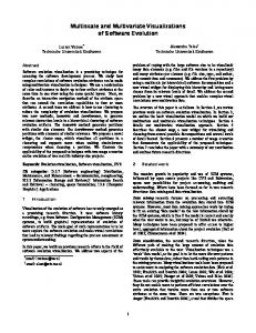
Version 3 The third version provided all the functionality of the second version, and also displayed the pseudocode of the algorithm. This enabled participants using this version to see how each individual line of the code affects the data set. Unlike the first version the participants were not provided with any example data set to work with.


30


Version 4 The fourth version used the same algorithm visualization as the second version (Figure 4.2) and also provided the participants with a (paper) reference material to make them explore the algorithm in a more detailed manner (Appendix A.2). This guide made the participants work through several examples, and required them to answer questions about the heapsort algorithm as they were working with it.

Version 5 The fifth version used the same visualization as the third version (Figure 4.3) and also provided the participants with the same (paper) reference material (Appendix A.2) that was used in the fourth version. The difference from the fourth version was the addition of the pseudocode display.

Features provided in each of the above five versions can be summarized as in the following table. Version 1

Version 2

Version 3

Version 4

Version 5

Next button Example dataset

Input Next button Back button

Input Pseudocode Next button Back button

Input Next button Back button Guide

Input Pseudocode Next button Back button Guide

Table 4.1: Feature list for the verisons

When the participants thought that they were sufficiently familiar with the algorithm, they were asked to answer questions (Appendix A.3) on the heapsort algorithm. Participants’ performance on the test would determine effectiveness of each algorithm visualization.

31


Question set The question set for Experiment 1 had 19 questions (Appendix A.3). We divided the questions into 3 groups to understand the results in a better way. We grouped questions 1 through 8 as conceptual questions. Questions 9 and 14 were categorized as pseudocode questions. Question 9 asked participants to identify pseudocode to form a max-heap. Question 14 asked participants to identify pseudocode for the heapsort algorithm. Remaining questions were grouped as procedural questions. Questions 10-13 asked participants to trace the steps of the algorithm to re-arrange the elements of a given array in a max-heap format and questions 15-19 asked participants to trace the steps of the algorithm to sort the elements of a given array once the first max-heap has been created.

4.2 Hypothesis We believed that since Version 1 had (relatively) minimum capabilities, participants would not be able to infer much about the heapsort algorithm from it. As Version 2 allowed participants to enter their own data set and also revert to a previous step in the algorithm, we believed that it would prove more helpful to understand the algorithm, as compared to the basic version. We believed that since Version 3 had a pseudocode display it would further increase participants’ understanding. As the reference material required participants to explore and analyze the algorithm in a detailed way we believed that Version 4 would prove more helpful than the earlier versions. We believed that the Version 5 would prove to be the most helpful.

4.3 Results 4.3.1

Total Performance

66 students participated in the experiment. We omitted the performance of 2 participants, as they had no prior knowledge about sorting, and thus they were quite different from the target population for use of the visualizations. The test (Appendix A.3) had 19 multiple-choice questions on the heapsort algorithm. We omitted the first question

32


in analysis as the background information provided the answer. On performing Anova analysis on the GPAs of participants of different groups there was no significant difference in average GPAs of different groups. There was no significant difference in the overall performance of the students. The average score for participants using Version 1 was the highest whereas average score for participants using Version 2 was the least. Anova analysis for the overall performance and average GPAs of the participants are included in Appendix A.5. 20 14.63636 15

12.07143

13.15385

13.28571

13.58333

2

3

4

5

10 5 0 1

Average Performance

Figure 4.4: Average Performance of participants

4.3.2

Individual Question Analysis

To further understand the results we analyzed performance of the participants on each individual question. Anova analysis on all the questions are included in Appendix A.5.

Conceptual Questions We categorized Questions 2 - 8 on the test (Appendix A.3) as conceptual questions. The following are questions on which a significant performance difference was found. Question 7 (Appendix A.3) asked participants about the memory requirements of the heapsort algorithm. Participants using Version 3 performed comparatively better as compared to other versions on this question. Anova analysis on performance of participants using Version 3 and Version 4 showed that participants using Version 3 performed significantly better than participants using Version 4 with a p value of 0.011.

33


1 0.765

0.8 0.6 0.4

0.3636

0.35

0.33 0.214

0.2 0 1

2

3

4

5

Average Performance on Q7

Figure 4.5: Average performance of participants on Q7

Question 8 (Appendix A.3) asked participants to identify the array in max-heap format from a set of given arrays.

Anova analysis on paired groups showed that

participants using Version 5 significantly outperformed participants using Version 2 with a p value of 0.00281 and participants using Version 4 with a p value of 0.0459. Participants using Version 1 outperformed participants using Version 2 with a p value of 0.029. 1.2 1 0.8 0.6 0.4 0.2 0

1

0.909091 0.769231

0.714286

3

4

0.5

1

2

5

Average Performance on Q8

Figure 4.6: Average performance of participants on Q8

Pseudocode Questions We categorized questions 9 and 14 on the test (Appendix A.3) as pseudocode questions. There was no significant difference in the performance of the participants using different versions on these questions.

34


Procedural questions We categorized Questions 10 through 13 and Questions 15 through 19 on the test (Appendix A.3) as procedural questions.

The following are questions on which a

significant performance difference was found. Questions 10 –13 asked participants to trace the steps of the heapsort algorithm to rearrange the elements of a given array in a max-heap format. Anova analysis showed that participants using Version 1 performed significantly better than participants using Version 3 with a p value of 0.00026, participants using version 4 with a p value of 0.0424 and participants using Version 5 with a p value of 0.0080. Participants using Version 4 and Version 2 performed significantly better than participants using Version 3with a p value of 0.0251 and 0.010 respectively. 1.2 1 0.8 0.6 0.4 0.2 0

1

0.928571

0.910714

0.854167

4

5

0.75

1

2

3 Average Performance on Q10-13

Figure 4.7: Average performance of participants on Q10-13

4.3.3

GPA Vs. Performance

Visualization of the GPA vs. Total score (shown in the figure below) shows no strong co-relation between GPA of the participants and their performance on the test. The data shown below is a scatter plot of GPA vs. Total performance of the participants using Spot fire (a data visualization tool). All the participants having a GPA = 12 on the test. For all other participants there is no strong co-relation between GPA and total performance.

35


Figure 4.8: Scatter Plot of GPA vs. Total Performance of the participants Participants having low GPAs but scoring above average

4.4 Conclusions

The overall performance indicates that participants using Version 1 performed somewhat better (not significantly) than participants using the other versions. On performing the individual question analysis, we can infer the reason for this. Participants using Version 1 significantly outperformed all the other participants (except Version 2) on procedural questions (Q 10-13). Participants using Version 2 or Version 4 performed significantly better than those using Version 3 on the procedural questions. Thus, from the results it can be inferred that a simple visualization that focuses just on the logical steps of an algorithm and shows its effect on the data would provide better understanding of the procedural steps of the algorithm to the participants who have no previous knowledge of the algorithm.

The results seem to indicate that a simple

visualization which focuses mainly on the procedural steps of the algorithm may help participants understand and notice the procedural steps in a better way. Too much information (like a pseudocode display, an activity guide) may over-whelm participants and thereby reduce the amount of procedural understanding they may gain from a visualization. It may also be possible that participants who observe a visualization that 36


focuses on procedural steps of an algorithm may be able to mimic the algorithm steps better and thereby obtain better results on the procedural questions than participants who have more amount of detail to work with. Also, working repeatedly with an example data set as in Version 1 which covers all the important cases in the algorithm may allow participants to understand the algorithm in a better way. The reason for this may be that participants who have no previous knowledge of algorithm do not know what would be a “good” data set to enter and therefore miss some of the important points in the algorithm. On Question 7 (Appendix A.3), which was a conceptual question, participants using Version 3 performed significantly better than participants using Version 4 and somewhat better (p = 0.087) than the participants using Version 2. On Question 8, another conceptual question (Appendix A.3), participants using Version 5 significantly outperformed participants using Version 2 or Version 4. Participants using Version 1 outperformed participants using Version 2. Participants using Version 3 outperformed participants using version 2. Thus, from the above results it can be inferred that a pseudocode display and an activity guide or a data example that covers all the important cases may provide better conceptual understanding of the algorithm. Participants who worked with Version 3 and Version 5 had a pseudocode of the algorithm displayed to them. Participants who worked with Version 5 were given an activity guide to work with (Appendix A.2) that made them analyze and answer questions about the algorithm, provided them with a few data sets to work with. Participants who had an activity guide usually spent more time with the visualization as compared to other participants as they had an activity guide to work with. This may have enabled them to understand the logic of the algorithm in a better way as compared to Versions 2 and Versions 4 who did not have a pseudocode display. However the results also inidcate another important point that an example data set may also help to provide conceptual understanding of the algorithm as the participants using either the Verison 3 or Version 5 did not perform better than Version 1.

37


The question set for Experiment 1 had two questions 9 and 14 (Appendix A.3) that asked participants pseudocode for the heapsort algorithm. We were surprised by the fact that the participants who had pseudocode display did not perform better on the pseudocode questions as compared to the participants who did not have a pseudocode display.

38

Chapter 5 Experiment 2 This chapter describes the second experiment that we conducted as a part of this thesis work. Our analysis of the first experiment gave counter-intuitive results (better performance by the basic version). We then hypothesized that two factors not tested for were dominating the results: having absolute control on the speed of algorithm execution and a data example. Thus, we did the second experiment to test this hypothesis. As in the first experiment, undergraduate students who had prior knowledge about simple sorting algorithms and knew basic data structures like stacks, queues, single linked lists, double linked lists, and circular linked lists, participated in this experiment. Most of these participants had no previous knowledge about the heapsort algorithm or the heap and tree data structures.

5.1 Procedure Participants were asked to work with one of four variations of the heapsort algorithm visualizations. All four variations used the same graphical representation of the algorithm and the same textual feedback messages used by all the visualizations in Experiment 1. Besides the algorithm visualization, participants were provided with some background information on the heapsort algorithm (Appendix A.1). For each participant, a log file that had a record of the time the participant spent with the visualization and also number of times that he/she interacted with various interface was maintained.


Version 1 Version 1 visualized the heapsort algorithm on a data set that the participants entered. Participants using this version were not given any example data set to work with. This version had a “next” button, but no “back” button, no pseudocode panel and no guide.


Version 2 Version 2 extended Version 1 by adding more capabilities to it. The participants using this version were provided with an example data set and could enter any other data set to visualize the algorithm. They were also able to revert to a previous step in the algorithm.

40



Version 3 Version 3 extended version 2 by adding more capabilities to it. The participants using this version were provided with a pseudocode display to show how each individual line of the heapsort algorithm code affects a given data set. Participants were able to revert to a previous step in the algorithm. Participants were provided with an example data set (same as Version 2) to begin the algorithm visualization. They could also enter any other data set. They were also provided with a paper reference material (Appendix A.2) to make them explore the algorithm in a more detailed way.

41



Version 4

Figure 5.4: Version 4 (Animation)

Unlike all the other visualizations created as a part of this thesis work, Version 4 animated the heapsort algorithm on a data set entered by the students. The participants using this version could control the speed of animation, but did not have a ‘Next’ button. Also as in Version 1 no example data set was provided to students.

42


Features provided in each of the above four versions can be summarized as in the following table. Version 1

Version 2

Version 3

Version 4

Input Next button

Input Example Next button Back button

Input Example Guide Pseudocode Next button Back button

Input Animation (No next button)

Table 5.1: Feature list for all versions.

When the participants thought that they were sufficiently familiar with the algorithm, they were asked to answer questions (Appendix A.4) about the heapsort algorithm. Participants performance on the test would determine the effectiveness of each Version.

Question set The results of Experiment 1 seem to indicate that participants who had a simple visualization that focused mainly on the logical steps of the algorithm performed better on procedural questions as compared to participants who had a pseudocode display or pseudocode display and activity guide. The results seem to suggest that participants who had more amount of detail presented to them (e.g. pseudocode display and activity guide) tend to perform worse on the procedural questions. To further analyse the results obtained from Experiment 1 we included more procedural questions in the question set for Experiment 2 as compared to the question set for Experiment 1. The question set for Experiment 2 had a total of 24 questions (Appendix A.4). We divided the questions into two groups: Conceptual and Procedural questions. Questions 1 through 5 were grouped as conceptual questions whereas the remaining questions were grouped as procedural questions. Questions 6–8 asked participants to rearrange a given array of 3 numbers in max-heap format. Questions 9-13 asked participants to rearrange an array of 4 numbers in a max-heap format. Questions 14-16 asked participants to sort an

43


array of 3 numbers after the first max-heap has been created. Questions 17-24 asked participants to sort an array of 4 numbers after the first max-heap has been created.

5.2 Hypothesis The results from the experiment 1 (Chapter 4) indicated that participants who used a minimal algorithm visualization (without many features) that focused mainly on the logical steps of the algorithm performed better on procedural questions. The results also indicated that a good data example and the pseudocode of an algorithm help in increasing students’ conceptual understanding of an algorithm. The results seem to indicate that providing a good example can prove to be most helpful to increase the pedagogical effectiveness of an algorithm visualization. To analyze the importance of a good data set (a data set that covers all the important cases in an algorithm) for conceptual understanding of the algorithm, participants were asked to study the heapsort algorithm with Version 1 and Version 2. Both the versions were almost identical except that participants using Version 2 were provided with a data example and could revert to a previous step in the algorithm. This would allow us to measure the difference in conceptual understanding of the two groups and determine if a good data set could increase the participants conceptual understanding of an algorithm. Version 3 used a pseudocode display, a data set example, and a guide that made students explore the algorithm in detail. By this, we wanted to see if providing all these features could further increase conceptual understanding of the algorithm. If Version 3 outperformed all the other versions on the conceptual questions, than based on the first and second experiment we would be able to conclude that providing additional features (like pseudocode and an activity guide) could increase students conceptual understanding of an unfamiliar algorithm. If there is a significant difference between performance of the students using Version 1 and Version 2 or Version 1 and Version 3 but no significant difference between the performance of students using Version 2 and Version 3, then we would conclude that providing a good data example can prove to be most helfpul in understanding the concept of an unfamiliar algorithm.

44


Results from Experiment 1 indicated that students who used minimal algorithm visualization (without many features) performed well on procedural questions. Also in Experiment 1 students who had a pseudocode display performed significantly worse on these questions. We should be able to analyze by comparing the performance of the students on questions 6-24 (Appendix A.4) using Version 1, Version 2 and Version 3, whether providing more features could result in reduced procedural understanding of the algorithm. Through this analysis we should also be able to understand the importance of providing a data set to understand the procedural steps of an algorithm. We also believed that allowing students to control the speed of algorithm execution would prove more helpful to understand an algorithm than showing an animation that does not provide absolute control on the algorithm execution. If our hypothesis was true then the students using Version 1 (Input) should perform better than students using Version 4 (animation). It is commonly assumed that the more time students spend with an algorithm visualization, the better understanding they have from the visualization. For the first experiment we did not measure the learning time (the amount of time students with the algorithm visualization) but for the second experiment we kept track of the learning time to know if there is any significant relation between the time students spend with the algorithm visualization and the score that they got on the test. Also, while creating the algorithm visualizations, many authors assume that it would help students if they could revert to a previous step in the algorithm visualization. We wanted to see if there was any specific relation between the usage of the history or the ‘back button’ and the scores students obtained on the test.

5.3 Results 5.3.1 Total Performance 44 Students, 11 for each version, participated in the experiment. The average GPAs of the participants of each group were almost similar. Anova analysis on the GPAs did not show any significant difference. The following is a bar chart showing average

45


performance of each version. The anova analysis for the total performance and GPAs of students is included in Appendix A.6. 22.27273

25 20

18.81818

16.63636

15

10.18182

10 5 0 1

2

3

4

Average Performance

Figure 5.5: Average performance of participants of each version.

The following is the summary of average performance of the participants Version 1 (Input Only) Version 2 (I +H+Ex) Version 3 (P+I+H+Ex+G) Version 4 (Animation)

Significantly worse than Version 2 (p=0.008) Significantly better than Version 1 (p=0.008) Non-significantly better than Version 1 (p=0. 35) Significantly worse than Version 1 (p = 0.029)

Non-significantly worse than Version 3 (p=0. 35) Non-significantly better than Version 3 (p=0.10) Non-significantly worse than Version 2 (p=0.107) Significantly worse than Version 2 (p=0.0001)

Significantly better than Version 4 (p = 0.03) Significantly better than version 4 (p=0.0001) Significantly better than Version 4 (p=0.006) Significantly worse than Version 3 (p=0.006)

Table 5.2: Summary of total performance.

The following is the partial ordering on the results for each version. The circular nodes represent each version (V1 = Version 1, V2 = Version 2, V3 = Version 3 and V4 = Version 4). The arrows are from the nodes (i.e. Version) that performed poor towards the nodes (i.e. Version) that had better performance.

The dotted arrows indicate non-

significant results where as a bold arrow indicates a significant performance difference.

46


V1

V2

V3

V4

Figure 5.6: Partial ordering on total performance of participants of each version.

As shown in the above table and partial order figure, participants who used Version 4 performed significantly worse than other participants. From this we can conclude that the providing an ability to control the pace of the visualization is very important. Participants using Version 2 performed significantly better than the participants using Version 1. From this we can conclude that providing a data set that covers all the important cases in an algorithm can prove to be pedagogically very effective.

5.3.2

Individual Question analysis

Anova analysis for the Individual questions are included in Appendix A.6.

Conceptual Questions Questions 1-5 (AppendixA.4): Participants using Versions 2 and 3 performed slightly better than those using Version 1 and Version 4 as shown by the average scores in the following bar char. However, on performing Anova analysis there was no significant performance difference.

47


5

4.636364

4.636364

2

3

4.272727

3.636364

4 3 2 1 0

1

4

Average Performance on Conceptual Questions

Figure 5.7 Average Performance on Conceptual Questions

Procedural questions Questions 6 – 24 on the test (Appendix A.4) were categorized as procedural questions.

On perfoming Anova analysis on performance on these questions we

discovered that participants using Version 2 performed significantly better than Version 1 (p=0.01479). Participants using Version 4 performed significantly worse than participants using all other versions p= 0.0139 as compared to Version 1, p= 0.000086 as compared to Version 2 and p= 0.0057 as compared to Version 3. 17.63636364

20 15

14.18181818

12.90909091

10

5.909090909

5 0 1

2

3

4

Average Performance on Procedural Questions Q6-24

Figure 5.8 Average Performance on Procedural Questions

The following is a summary of the results on Anova analysis for individual procedural questions.

48


Questions 6-8 (Appendix A.4) asked students to trace the steps of the heapsort algorithm to rearrange a given array having 3 numbers in max-heap format. Participants using Version 1 performed significantly (p=0.02678) better than Version 4. 3.5 3 2.5 2 1.5 1 0.5 0

3 2.454545

2.272727 1.727273

1

2

3

4

Average Performance on Q6-8

Figure 5.9: Average performance of the participants on Q 6-8.

Questions 9-13 (Appendix A.4) asked students to trace the steps of the heapsort algorithm to re-arrange a given array of 4 numbers in a max-heap format. Participants using Version 2 performed significantly better than participants using Version 1 (p=0.009). Participants using Version 2 and Version 3 performed significantly better than participants using Version 4 with p=0.0006 and p=0.008 respectively. 5

6 4

4.545455

2.727273

2

2 0 1

2

3

4


Figure 5.10: Average performance of the participants on Q 9-13.

Questions 14 – 16 (Appendix A.4) asked students to trace steps of the heapsort algorithm to sort a given array of 3 elements after the first max-heap has been created. The participants using Version 4 performed worse than all other versions with p=0.03, p=4.030E-06, and p=0.008 as compared to Version 1, Version 2 and Version 3

49


respectively. Participants using Version 2 also performed significantly better than participants using Version 1 with p=0.02. 3.5 3 2.5 2 1.5 1 0.5 0

2.909091 2.181818 1.818182 0.545455

1

2

3

4


Figure 5.11: Average Performance of participants on Q14-16.

Questions 17- 24 (Appendix A.4) asked participants to trace steps of the heapsort algorithm to sort elements of a given array of 4 numbers after the first max-heap has been created. Participants using Version 4 performed significantly worse than participants using than participants using Version 1with p=0.016 and those using Version 2 with p=0.0001. Participants using Version 2 performed marginally better than participants using Version 3 (p=0.059). 7.272727

8 5.363636

6

4.363636

4 1.454545

2 0 1

2

3

4


Figure 5.12: Average Performance on participants on Q17-24.

The above results on the pseudocode questions can be summarized as in the following table.

50


Questions 6 -8 Questions 9-13

Questions 14-16

Questions 17-24

Version 1 performed better than version 4. Participants Participants Participants using Version 2 using Version 2 using Version 3 performed performed performed significantly significantly significantly better (p = better (p= better than those 0.009) than 0.0006) than using Version 4 those using those using (p=0.008) Version 1 Version 4 Participants Participants Participants using Version 1 using Version 2 using Version 2 performed performed performed significantly significantly significantly better (p= 0.03) better better than (p=0.020) than (p=4.030E-06) participants participants than participants using Version 4 using Version 1 using Version 4.

Participants using Version 3 performed marginally better than those using Version 1 (p=0.059). Participants using Version 3 performed significantly better (p=0.008) than those using Version 4.

Participants using Version 1 performed significantly (p= 0.016) better than the participants using Version 4

Participants using Version 3 performed marginally better than those using Version 4 (p= 0.0828).

Participants using Version 2 performed significantly better than the participants using Version 4 (p= 0.0001

Participants using Version 2 performed marginally better than those using Version 3 (p= 0.0592).

Table 5.3: summary of performance on individual questions.

5.3.3

Performance vs. Learning Time

The following is a scatter plot of Learning Time Vs. Average Performance. As shown in the below scatter plot, more time spent with the visualization does not imply that students would have better understanding of the algorithm. Participants using Version 3 spent about 41.73 minutes studying the applet and working with the guide, however this did not result in better scores than the participants using Version 2 who spent only an average of 18.73 minutes with the visualization.

51


V4

V1

V2

Figure 5.13: Average learning time vs. Average Scores. Participants using Version 3 more than double time as compared to other versions.

Version 1 The following figure is a scatter plot of Learning time vs. Performance of participants using Version 1 in Spot fire. As shown in the figure below, the learning time did not affect the performance.

Figure 5.14: A scatter plot of Learning time vs. Performance for participants using Version1 using Spot fire.

52


Version 2 As shown in the figure below, the learning time did not have any significant effect on performance of participants using Version 2. The following is a scatter plot of Learning time vs. Performance of participants using Version 2 in Spot fire.

Figure 5.15: A scatter plot of Learning time vs. Performance for participants using Version 2 using Spot fire.

Version 3 Like the previous two versions, there was no relation between learning time and performance of the participants.

53



Version 4 Again there was no correlation between learning time and performance for participants using Version 4.


5.3.4

GPA vs. Performance

The following figure shows a scatter plot of GPA vs. Total performance of participants. No strong correlation is seen between GPA of participants and their 54


performance. However, it is interesting to note that all the 3 participants having low GPA (

Effective Features of Algorithm Visualizations - CiteSeerX

Effective Features of Algorithm Visualizations - CiteSeerX

Suggest Documents

Effective Features of Algorithm Visualizations - CiteSeerX

Designing Effective Visualizations for Elementary School ... - CiteSeerX

Specifying Algorithm Visualizations in Terms of Data Flow - CiteSeerX

Specifying Algorithm Visualizations - Georgia Tech College of

Towards Effective Interaction in 3D Data Visualizations - CiteSeerX

Designing Effective Visualizations for Elementary School Science

Using algorithm visualizations in computer science ...

Critical Features of Visualizations of Transport ... - Semantic Scholar

Fluency of visualizations: linking spatiotemporal visualizations to ...

The Power of Geographical Visualizations - CiteSeerX

Glyphmaker: creating customized visualizations of ... - CiteSeerX

VisFlowConnect: NetFlow Visualizations of Link ... - CiteSeerX

Multiscale and Multivariate Visualizations of Software ... - CiteSeerX

Comparison of Path Visualizations and Cognitive ... - CiteSeerX

Boundary/Contour Fitted Grid Generation for Effective Visualizations in ...

Towards Effective Interaction in 3D Data Visualizations - Core

From B-Spline Mesh Generation to Effective Visualizations for the ...

Searching for Features using a Genetic Algorithm - CiteSeerX

Contextualized Text Explanations for Visualizations - CiteSeerX

Designing Task Visualizations to Support the ... - CiteSeerX

Creating visualizations through ontology mapping - CiteSeerX

Automatically Generating Summary Visualizations from ... - CiteSeerX

features - CiteSeerX

Features - CiteSeerX