Effective Representation of Aliases and Indirect Memory ... - CiteSeerX

Effective Representation of Aliases and Indirect Memory Operations in SSA Form Fred Chow, Sun Chan, Shin-Ming Liu, Raymond Lo, Mark Streich Silicon Graphics Computer Systems 2011 N. Shoreline Blvd. Mountain View, CA 94043

Contact: Fred Chow (E-mail: [email protected], Phone: USA (415) 933-4270) Abstract. This paper addresses the problems of representing aliases and indirect memory operations in SSA form. We propose a method that prevents explosion in the number of SSA variable versions in the presence of aliases. We also present a technique that allows indirect memory operations to be globally commonized. The result is a precise and compact SSA representation based on global value numbering, called HSSA, that uniformly handles both scalar variables and indirect memory operations. We discuss the capabilities of the HSSA representation and present measurements that show the effects of implementing our techniques in a production global optimizer. Keywords. Aliasing, Factoring dependences, Hash tables, Indirect memory operations, Program representation, Static single assignment, Value numbering.

1 Introduction The Static Single Assignment (SSA) form [CFR+91] is a popular and efficient representation for performing analyses and optimizations involving scalar variables. Effective algorithms based on SSA have been developed to perform constant propagation, redundant computation detection, dead code elimination, induction variable recognition, and others [AWZ88, RWZ88, WZ91, Wolfe92]. But until now, SSA has only been used mostly for distinct variable names in the program. When applied to indirect variable constructs, the representation is not straight-forward, and results in added complexities in the optimization algorithms that operate on the representation [CFR+91, CG93, CCF94]. This has prevented SSA from being widely used in production compilers. In this paper, we devise a scheme that allows indirect memory operations to be represented together with ordinary scalar variables in SSA form. Since indirect memory accesses also affect scalar variables due to aliasing, we start by defining notations to model the effects of aliasing for scalars in SSA form. We also describe a technique to reduce the overhead in SSA representation in the presence of aliases. Next, we introduce the concept of virtual variables, which model indirect memory operations as if they are scalars. We then show how virtual variables can be used to derive identical or distinct versions for indirect memory operations, effectively putting them in SSA form together with the scalar variables. This SSA representation in turn reduces the cost of analyzing the scalar variables that have aliases by taking advantage of the versioning applied to the indirect memory operations aliased with the scalar variables. We then present a method that builds a uniform SSA representation of all the scalar and indirect

1

memory operations of the program based on global value numbering, which we call the Hashed SSA representation (HSSA). The various optimizations for scalars can then automatically extend to indirect memory operations under this framework. Finally, we present measurements that show the effectiveness of our techniques in a production global optimizer that uses HSSA as its internal representation. In this paper, indirect memory operations cover both the uses of arrays and accesses to memory locations through pointers. Our method is applicable to commonly used languages like C and FORTRAN.

2 SSA with Aliasing In our discussion, the source program has been translated to an intermediate representation in which expressions are represented in tree form. The expression trees are associated with statements that use their computed results. In SSA form, each definition of a variable is given a unique version, and different versions of the same variable can be regarded as different program variables. Each use of a variable version can only refer to a single reaching definition. When several definitions of a variable, a1, a2, ..., am, reach a confluence node in the control flow graph of the program, a φ function assignment statement, an = φ(a1, a2, ..., am), is inserted to merge them into the definition of a new variable version an. Thus, the semantics of single reaching definitions is maintained. This introduction of a new variable version as the result of φ factors use-def edges over confluence nodes, reducing the total number of use-def edges required. As a result, the use-def chain of each variable can be provided in a compact form by trivially allowing each variable to point to its single definition. One important property in SSA form is that each definition must dominate all its uses in the control flow graph of the program. Another important property in SSA form is that identical versions of the same variable must have the same value. Aliasing of a scalar variable occurs in one of four conditions: when its storage location partially overlaps another variable1, when it is pointed to by a pointer used in indirect memory operations, when its address is passed in a procedure call, or when it is a non-local variable that can be accessed from another procedure in a call or return. Techniques have been developed to analyze pointers both intra-procedurally and inter-procedurally to provide more accurate information on what is affected by them so as to limit their ill effects on program optimizations [CWZ90, CBC93, Ruf95, WL95]. To characterize the effects of aliasing, we distinguish between two types of definitions of a variable: MustDef and MayDef.2 Since a MustDef must redefine the variable, it blocks the references of previous definitions from that point on. A MayDef only potentially redefines the variable, and so does not prevent previous definitions of the

1. If they exactly overlap, our representation will handle them as a single variable. 2. In [CCF94], MustDefs and MayDefs are called Killing Defs and Preserving Defs respectively, while in [Steen95], they are called Strong Updates and Weak Updates.

2

SSA Representation: i1 ← 2 if (j1)

Original Program: i←2 if (j)

µ(i1)

*p ← 3

call func()

call func()

*p ← 3

i2←χ(i1)

i3←φ(i1, i2)

return i

return i3

Fig. 1. Example of µ, χ and φ same variable from being referenced later in the program. On the use side, in addition to real uses of the variable, there are places in the program where there are potential references to the variable that need to be taken into account in analyzing the program. We call these potential references MayUse. To accommodate the MayDefs, we use the idea from [CCF94] in which SSA edges for the same variable are factored over its MayDefs. This is referred to as location-factored SSA form in [Steen95]. We model this effect by introducing the χ assignment operator in our SSA representation. χ links up the use-def edges through MayDefs. The operand of χ is the last version of the variable, and its result is the version after the potential definition. Thus, if variable i may be modified, we annotate the code with i2 = χ(i1), where i1 is the current version of the variable. To model MayUses, we introduce the µ operator in our SSA representation. µ takes as its operand the version of the variable that may be referenced, and produces no result. Thus, if variable i may be referenced, we annotate the code with µ(i1), where i1 is the current version of the variable. In our internal representation, expressions cannot have side effects. Memory locations can only be modified by statements, which include direct and indirect store statements and calls. Thus, χ can only be associated with store and call statements. µ is associated with any dereferencing operation, like the unary operator * in C, which can happen within an expression. Thus, µ arises at both statements and expressions. We also mark return statements with µ for non-local variables to represent their liveness at function exits. Separating MayDef and MayUse allows us to model the effects of calls precisely. For example, a call that only references a variable will only cause a µ but no χ. For our modeling purpose, the µ takes effect just before the call, and the χ takes effect right after the call. Figure 1 gives an example of the use of µ, χ together with φ in our SSA representation. In the example, function func uses but does not modify variable i. The inclusion of µ and χ in the SSA form does not impact the complexity of the algorithm that computes SSA form. A pre-pass inserts unnamed µ’s and χ’s for the

3

aliased variables at the points of aliases in the program. In applying the SSA creation algorithm described in [CFR+91], the operands of the µ and χ are treated as uses and the χ’s are treated as additional assignments. The variables in the µ and χ are renamed together with the rest of the program variables. Transformations performed on SSA form have to take aliasing into account in order to preserve the safety of the optimization. In our SSA representation, it means taking into account the µ and χ annotations. For example, in performing dead code elimination using the algorithm presented in [CFR+91], a store can be deleted only if the store itself and all its associated χ’s are not marked live.

3 SSA with Zero Versioning In the previous section, we showed how to use µ and χ to model use-def information when aliases occur in a program. Even though use-def information is maintained, the number of versions multiplies because each χ introduces a new version and it may in turn cause new φ’s to be inserted. Many of these versions have multiple possiblydefined values, and some of the defined values may also be unknown. As a result, it becomes relatively more expensive to represent programs in SSA form in the presence of aliases. In this section, we describe a technique to alleviate this problem. We call occurrences of variables in the original program before conversion to SSA form real occurrences. In SSA form, variable occurrences in φ, µ and χ are thus not real occurrences. The variable versions that have no real occurrence do not directly affect the optimized output of the program once the program is converted back to ordinary form. But they do indirectly affect the optimizations that follow use-def chains that pass through φ, µ and χ. Once identified, these variable versions that have no real occurrence can be aggregately represented by a special version of the variable, thus reducing the number of versions of the variable that need to be represented, with only a slight impact on the quality of the optimized output. For the purpose of our discussion, we assign version 0 to this special version, and call it the zero version. Definition 1. The zero versions are versions of variables that have no real occurrence and whose values come from at least one χ with zero or more intervening φ’s. Alternatively, we can define zero versions recursively as follows: 1. The left hand side of a χ is zero version if it has no real occurrence. 2. If an operand of a φ is zero version, the result of the φ is zero version if it has no real occurrence. Zero versioning thus characterizes versions with no real occurrence whose values are affected by aliased stores. Since their values are not fixed, we do not assign unique versions to them and do not represent their use-def relationships. We now give the algorithm to compute zero versions. We assume all variables have been renamed in the process of building the SSA form. Our algorithm assumes that defuse information, which is more expensive than use-def under SSA, is not maintained,

4

and only use-def information is available.1The algorithm identifies the versions of variables that can be made zero-version and resets their versions to 0. Algorithm 1. Compute Zero Versions: 1. Initialize flag HasRealOcc for each variable version created by SSA renaming to false. 2. Pass over the program. On visiting a real occurrence, set the HasRealOcc flag for the variable version to true.2 3. For each program variable, create NonZeroPhiList and initialize to empty. 4. Iterate through all variable versions: a. If HasRealOcc is false and it is defined by χ, set version to 0. b. If HasRealOcc is false and it is defined by φ: • If the version of one of the operands of the φ is 0, set version to 0. • Else if the HasRealOcc flag of all of the operands of the φ is true, set HasRealOcc to true. • Else add version to NonZeroPhiList for the variable. 5. For each program variable, iterate until its NonZeroPhiList no longer changes: a. For each version in NonZeroPhiList: • If the version of one of the operands of the φ is 0, set version to 0 and remove from NonZeroPhiList. • Else if the HasRealOcc flag of all the operands of the φ is true, set HasRealOcc to true and remove from NonZeroPhiList. The first iteration through all the variable versions, represented by Step 4, completely processes all variable versions except those that are the results of φ whose operands have not yet been processed. These are collected into NonZeroPhiList. After the first iteration of Step 5, the versions still remaining in NonZeroPhiList all have at least one operand defined by φ. The upper bound on the number of iterations in Step 5 corresponds to the longest chain of contiguous φ assignments for the variable in the program. When no more zero versions can be propagated through each φ, the algorithm terminates. Because zero versions can have multiple assignments statically, they do not have fixed or known values, so that two zero versions of the same variable cannot be assumed to be the same. The occurrence of a zero version breaks the use-def chain. Since the results of χ’s have unknown values, zero versions do not affect the performance of optimizations that propagate known values, like constant propagation [WZ91], because they cannot be propagated across points of Maydefs to the variables. Optimizations that

1. If def-use information is present, a more efficient algorithm is possible. 2. The pass to set the HasRealOcc flag can coincide with another pass over the program that performs an unrelated optimization, e.g. dead store elimination.

5

a←

a1 ←

a1 ←

µ(a1) call func() a2 ← χ(a1)

call func()

µ(a1) call func() a0 ← χ(a1)

a3 ←φ(a1, a2)

a0 ←φ(a1, a0)

µ(a3) return

µ(a0) return

return

(a) Original Program (b) SSA form (b) SSA form with 0 versions Fig. 2. Example of Using Zero Versions operate on real occurrences, like equivalencing and redundancy detection [AWZ88, RWZ88], are also unaffected. In performing dead store elimination, zero versions have to be assumed live. Since zero versions can only have uses represented by µ’s, the chance that stores associated with χ’s to zero versions can be removed is small. However, it is possible that later optimizations delete the code that contains the µ’s. Only in such situations would zero version prevent more dead store elimination. Zero versions are created only when aliases occur. Our approach does not affect optimization when there is no aliasing. Zero versioning also does not prevent the SSA form from being used as a representation for various program transformations, because it is not applied to real occurrences. When aliases are prevalent in the program, zero versioning prevents the number of variable versions in the SSA form from exploding. In the example of Figure 2, since a is a global variable, it has a µ at the return statement. Our algorithm eliminates versions a2 and a3 by converting them to version 0.

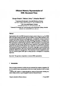
4 SSA for Indirect Memory Operations In an indirect memory operation, the memory location referenced depends on the values of the variables involved in the computation specified by the address expression. Figure 3 gives examples of indirect memory operations and their tree representation. Indirect memory operations are either indirect loads or indirect stores. We refer to them as loads and stores to indirect variables, as opposed to scalar variables. Indirect variables are identified by the form of their address expressions. We use the C dereferencing operator Source construct:

*p

Tree representation:

*

**p

*(p+1)

p p

p->next

a[i]

*

*

*

*

+

*

+

+

1

p p Fig. 3. Examples of Indirect Memory Operations

6

8

&a

i

Original Program:

SSA Representation:

. . *p . .

. . (*p1)1 . .

p←p+1

p2 ← p1 + 1 . . (*p2)2 . .

. . *p . . Fig. 4. Renaming Indirect Variables

* to denote indirection. Given an address expression , * represents a load of the indirect variable and ∗ ← represents a store to the indirect variable. We can apply the same algorithm that computes SSA form for scalar variables to indirect variables, renaming them such that versions that statically have the same value get the same name. The difference is that each indirect variable needs to be treated as separate indirect variables if the variables involved in their address expressions are not of identical versions. This is illustrated in Figure 4, in which the two occurrences of *p are renamed to different versions. Though *p is not redefined between the two occurrences, p is redefined. The obvious way to tackle the above problem is to apply the algorithm to compute SSA form multiple times to a program. The first application computes the versions for all scalar variables, the second application computes the versions for all indirect variables with one level of indirection, the third application computes the versions for all indirect variables with two levels of indirection, etc. Multiple invocation of the SSA computation algorithm would be prohibitively expensive and not practical. The only advantage with this approach is that, in between each application, it is possible to improve on the alias analysis by taking advantage of the version and thus use-def information just computed in the address expression. We have formulated a scheme that allows us to compute the SSA form for all scalar and indirect variables in one pass. For this purpose, we introduce virtual variables to characterize indirect variables and include them in computing the SSA form. Definition 2. The virtual variable of an indirect variable is an imaginary scalar variable that has identical alias characteristics as the indirect variable. For all indirect variables that have similar alias behavior in the program, we assign a unique virtual variable. We use v superscripted with the indirect variable name to denote a virtual variable. Alias analysis is performed on the virtual variables together with the scalar variables. For virtual variables, alias analysis can additionally take into account the form of the address expression to determine when they are independent. For example, v*p and v*(p+1) do not alias with each other. We then apply the algorithm to compute SSA form for all the scalar and indirect variables of the program. Since each virtual variable aliases with its indirect variable, the resulting SSA representation must have each occurrence of an indirect variable annotated with µ or χ of its virtual variable. The use-def relationship in the virtual variable now represents the use-def relationship of its

7

a[i] ←

(a[i1])1 ←

(a[i1])1 ←

v*2←χ(v*1)

*p ←

(*p1)1 ←

i ←i + 1

i2 ← i1 + 1

v*3←χ(v*2)

(*p1)1 ← v*p2←χ(v*p1)

i2 ←i1 + 1 i3 ←φ(i1, i2)

i3 ←φ(i1, i2) v*4 ←φ(v*2, v*3)

. . a[i] . .

va[i]2←χ(va[i]1)

v*p3 ←φ(v*p1, v*p2) µ(va[i]2)

µ(v*4)

. . (a[i3])2 . .

. . (a[i3])2 . .

(3 versions of v*p, 2 versions of va[i]) (b) Using 1 virtual variable v* (c) Using 2 virtual variables (a) Original Program va[i] and v*p Indirect variables a[i] and *p do not alias with each other (4 versions of v*)

Fig. 5. SSA for indirects using different numbers of virtual variables indirect variable. Each occurrence of a indirect variable can then be given the version number of the virtual variable that annotates it in the µ or χ, except that new versions need to be generated when the address expression contains different versions of variables. We can easily handle this by regarding indirect variables whose address expressions have been renamed differently to be different indirect variables, even though they share the same virtual variable due to similar alias behavior. In Figure 4, after p has been renamed, *p1 and *p2 are regarded as different indirect variables. This causes different version numbers to be assigned to the *p’s, (*p1)1 and (*p2)2, even though the version of the virtual variable v*p has not changed. It is possible to cut down the number of virtual variables by making each virtual variable represent more indirect variables. This is referred to as assignment factoring in [Steen95]. It has the effect of replacing multiple use-def chains belonging to different virtual variables with one use-def chain that has more nodes and thus versions of the virtual variable, at the expense of higher analysis cost while going up the use-def chain. In the extreme case, one virtual variable can be used to represent all indirect variables in the program. Figure 5 gives examples of using different numbers of virtual variables in n a program. In that example, a[i1] and a[i2] are determined to be different versions because of the different versions of i used in them, and we assign versions 1 and 2 (shown as subscripts after the parentheses that enclose them) respectively. In part (b) of Figure 5, when we use a single virtual variable v* for both a[i] and p, even though they

8

do not alias with each other, the single use-def chain has to pass through the appearances of both of them, and is thus less accurate. In practice, we do not use assignment factoring among variables that do not alias among themselves, so that we do not have to incur the additional cost of analyzing the alias relationship between different variables while traversing the use-def chains. For example, we assign distinct virtual variables to a[i] and b[i] where arrays a and b do not overlap with each other. While traversing the use-def chains, we look for the presence of non-aliasing in indirects by analyzing their address expressions. For example, a[i1] does not alias with a[i1+1] even though they share the same virtual variable. Zero versions can also be applied to virtual variables, in which virtual variables appearing in the µ and χ next to their corresponding indirect variables are regarded as real occurrences. This also helps to reduce the number of versions for virtual variables.

5 Global Value Numbering for Indirect Memory Operations In this section, we apply the various ideas presented in this paper to build a concise SSA representation of the entire program based on global value numbering (GVN). We call our representation Hashed SSA (HSSA) because of the use of hashing in value numbering. HSSA serves as the internal program representation of our optimizer, on which most optimizations are performed. Value numbering [CS70] is a technique to recognize expressions that compute the same value. It uses a hash table to store all program expressions. Each entry in the hash table is either an operand (leaf) or an operator (internal) node. The hash table index of each entry corresponds to its unique value number. The value number of an internal node is a function of the operator and the value numbers of all its immediate operands. Any two nodes with the same value number must compute the same value. Value numbering yields a directed acylic graph (DAG) representation of the expressions in the program. Without SSA form, value numbering can only be performed at the basic block level, as in [Chow83]. SSA enables value numbering to be performed globally. The representation is more compact, because each variable version maps to a unique value number and occupies only one entry in the hash table, no matter how many times it occurs in the program1. Expressions made up of variables with identical versions are represented just once in the hash table, regardless of where they are located in the control flow graph. In value numbering, when two indirect memory operations yield the same hash value, they may not be assigned the same value number because the memory locations may contain different values. In straight-line code, any potential modification to the memory location can be detected by monitoring operations that affect memory while

1. The identification of each variable version is its unique node in the hash table, and the version number can be discarded.

9

traversing the code. But with GVN, this method cannot be used because GVN is flowinsensitive. One possibility is to give up commonizing the indirect operators by always creating a new value number for each indirect operator. This approach is undesirable, since it decreases the optimality and effectiveness of the GVN. To solve this problem, we apply the method described in the previous section of renaming indirect operations. During GVN, we map a value number to each unique version of indirect operations that our method has determined. Our GVN has some similarity to that described in [Click95], in that expressions are hashed into the hash table bottom-up. However, our representation is in the form of expression trees, instead of triplets. Since we do not use triplets, variables are distinct from operators. Statements are not value-numbered. Instead, they are linked together on a per-block basis to represent the execution flow of each basic block. The DAG structure allows us to provide use-def information cheaply and succinctly, via a single link from each variable node to its defining statement. The HSSA representation by default does not provide def-use chains. Our HSSA representation has five types of nodes. Three of them are leaf nodes: const for constants, addr for addresses and var for variables. Type op represents general expression operators. Indirect variables are represented by nodes of type ivar. Type ivar is a hybrid between type var and type op. It is like type op because it has an expression associated with it. It is like type var because it represents memory locations. The ivar node corresponds to the C dereferencing operator *. Both var and ivar nodes have links to their defining statements. We now outline the steps to build the HSSA representation of the program: Algorithm 2. Build HSSA: 1. Assign virtual variables to indirect variables in the program. 2. Perform alias analysis and insert µ and χ for all scalar and virtual variables. 3. Insert φ using the algorithm described in [CFR+91], including the χ as assignments. 4. Rename all scalar and virtual variables using the algorithm described in [CFR+91]. 5. Perform the following simultaneously: a. Perform dead code elimination to eliminate dead assignments, including φ and χ, using the algorithm described in [CFR+91]. b. Perform Steps 1 and 2 of the Compute Zero Version algorithm described in Section 3 to set the HasRealOcc flag for all variable versions. 6. Perform Steps 3, 4 and 5 of the Compute Zero Version algorithm to set variable versions to 0. 7. Hash a unique value number and create the corresponding hash table var node for each scalar and virtual variable version that are determined to be live in Step 5a. Only one node needs to be created for the zero versions of each variable.

10

8. Conduct a pre-order traversal of the dominator tree of the control flow graph of the program and apply global value numbering to the code in each basic block: a. Hash expression trees bottom up into the hash table, searching for any existing matching entry before creating each new value number and entry. At a var node, use the node created in Step 7 for that variable version. b. For two ivar nodes to match, two conditions must be satisfied: (1) their address expressions have the same value number, and (2) the versions of their virtual variables are either the same, or are separated by definitions that do not alias with the ivar. c. For each assignment statement, including φ and χ, represent its left hand side by making the statement point to the var or ivar node for direct and indirect assignments respectively. Also make the var or ivar node point back to its defining statement. d. Update all φ, µ and χ operands and results to make them refer to entries in the hash table. The second condition of Step 8b requires us to go up the use-def chain of the virtual variable starting from the current version to look for occurrences of the same ivar node that are unaffected by stores associated with the same virtual variable. For example, a store to a[i1+1] after a use of a[i1] does not invalidate a[i1]. Because we have to go up the use-def chain, processing the program in a pre-order traversal of the dominator tree of the control flow graph guarantees that we have always processed the earlier definitions. Once the entire program has been represented in HSSA form, the original input program can be deleted. Figure 6 gives a conceptual HSSA representation for the example of Figure 4. In our actual implementation, each entry of the hash table uses a linked list

Hash Table

Value Number

2 3

Statement

lhs = 3

def

: 11

const 1

24

ivar

kid1 = 2

op +

kid1 = 2

ivar

kid1 = 3

: :

Store

var p var p

rhs = 42

: 42

: 55

:

Fig. 6. HSSA representation for the example in Figure 5

11

kid2 = 11

for all the entries whose hash numbers collide, and the value number is represented by the pair .

6 Using HSSA The HSSA form is more memory efficient than ordinary representations because of structure sharing resulting from DAGs. Compared to ordinary SSA form, HSSA also uses less memory because it does not provide def-use information, while use-def information is much less expensive because multiple uses are represented by a common node. Many optimizations can run faster on HSSA because they only need to be applied just once on the shared nodes. The various optimizations can also take advantage of the fact that it is trivial to check if two expressions compute the same value in HSSA. An indirect memory operation is a hybrid between expression and variable, because it is not a leaf node but operates on memory. Our HSSA representation captures this property, so that it can benefit from optimizations applied to either expressions or variables. Optimizations developed for scalar variables in SSA form can now be applied to indirect memory operations. With the use-def information for indirect variables, we can substitute indirect loads with their known values, performing constant propagation or forward substitution. We can recognize and exploit equivalences among expressions that include indirect memory operations. We can also remove useless direct and indirect stores at the same time while performing dead code elimination. The most effective way to optimize indirect memory operations is to promote them to scalars when possible. We call this optimization indirection removal, which refers to the conversion of an indirect store and its subsequent indirect loads to direct store and loads. This promotion to scalar form enables it to be allocated to register, thus eliminating accesses to memory. An indirect variable can be promoted to a scalar whenever it is free of aliases. This can be verified by checking for the presence of its virtual variables in µ’s and χ’s. Promotion of an ivar node can be effected by overwriting it with the contents of the new var node, thus avoiding rehashing its ancestor nodes in the DAG representation. Optimization opportunites in indirect memory operations depends heavily on the quality or extent of alias analysis. Implementing the above techniques in an optimizer enables programs to benefit directly from any improvement in the results of the alias analyzer.

7 Measurements We now present measurements that show the effects of applying the techniques we described in this paper. The measurements are made in the production global optimizer WOPT, a main component of the compiler suite that will be shipped on MIPS R10000based systems in May of 1996. In addition to the optimizations described in Section 6,

12

Routine tomcatv

Language FORTRAN

Description 101.tomcatv, SPECfp95

loops

FORTRAN

subroutine loops from 103.su2cor, SPECfp95

kernel

FORTRAN

routine containing the 24 Lawrence Livermore Kernels

twldrv

FORTRAN

subroutine twldrv from 145.fpppp, SPECfp95

Data_path

C

function Data_path from 124.m88ksim, SPECint95

compress

C

function compress from 129.compress, SPECint95

Query_Ass

C

function Query_AssertOnObject from 147.vortex, SPECint95

eval

C

function eval from 134.perl, SPECint95

Table 1. Description of routines used in measurements WOPT also performs bit-vector-based partial redundancy elimination and strength reduction. From the input program, it builds HSSA and uses it as its only internal program representation until it finishes performing all its optimizations. We focus on the effects that zero versioning and the commonizing of indirect variables have on the HSSA representation in the optimizer. We have picked a set of 8 routines, 7 of which are from the SPEC95 benchmark suites. Table 1 describes these routines. We have picked progressively larger routines to show the effects of our techniques as the size of the routines increases. The numbers shown do not include the effects of inter-procedural alias analysis. We characterize the HSSA representation by the number of nodes in the hash table needed to represent the program. The different types of nodes are described earlier in Section 5. Without zero versioning, Table 2 shows that var nodes can account for up to 94% of all the nodes in the hash table. Applying zero versioning decreases the number of var nodes by 41% to 90%. The numbers of nodes needed to represent the programs are reduced from 30% to 85%. Note that the counts for non-var nodes remain constant, since only variables without real occurrences are converted to zero versions. Having to deal with less nodes, the time spent in performing global optimization is reduced from 2% to 45%. The effect of zero versioning depends on the amount of aliasing in the program. Zero versioning also has bigger effects on large programs, since there are more variables affected by each alias. We have found no noticeable difference in the running time of the benchmarks due to zero versioning. With zero versioning being applied, Table 3 shows the effects of commonizing indirect variables on the HSSA representation. Ivar nodes account for from 6% to 21% of the total number of nodes in our sample programs. Commonizing ivar nodes reduces the ivar nodes by 3% to 58%. In each case, the total number of nodes decreases more than the number of ivar nodes, showing that commonizing the ivar nodes in turn enables other operators that operate on them to be commonized. Though the change in the total number of hash table nodes is not significant, the main effect of this technique is in preventing missed optimizations, like global common subexpressions, among indirect memory operations.

13

number of nodes routines

tomcatv

zero version off

percentage reduction

zero version on

all

vars

all

vars

all

vars

1803

1399

844

440

53%

69%

compilation speedup 4%

loops

7694

6552

2493

1351

68%

79%

9%

kernel

9303

8077

2974

1748

68%

78%

6%

twldrv

33683

31285

6297

3899

81%

88%

11%

489

365

340

216

30%

41%

2%

Data_path compress

759

647

367

255

52%

61%

4%

Query_Ass

5109

4653

1229

773

76%

83%

12%

eval

62966

59164

9689

5887

85%

90%

45%

Table 2. Effects of zero versioning number of nodes percentage reduction routines

ivar commoning off all nodes

ivar nodes

tomcatv

844

124

loops

2493

453

kernel

2974

398

twldrv

6297

506

ivar commoning on all nodes

ivar nodes

all nodes

ivar nodes

828

111

2%

10%

2421

381

3%

16%

2854

306

4%

23%

6117

333

3%

34%

Data_path

340

44

320

30

6%

32%

compress

367

21

365

19

0.5%

10%

Query_Ass

1229

183

1218

173

1%

5%

eval

9689

1994

9114

1504

6%

25%

Table 3. Effects of the global commonizing of ivar nodes

8 Conclusion We have presented practical methods that efficiently model aliases and indirect memory operations in SSA form. Zero versioning prevents large variations in the representation overhead due to the amount of aliasing in the program, with minimal impact on the quality of the optimizations. The HSSA form captures the benefits of SSA while efficiently representing program constructs using global value numbering. Under HSSA, the integration of alias handling, SSA and global value numbering enables indirect memory operations to be globally commonized. Generalizing SSA to indirect memory operations in turn allows them to benefit from optimizations developed for scalar variables. We believe that these are all necessary ingredients for SSA to be used in a production-quality global optimizer.

14

Acknowledgement The authors would like to thank Peter Dahl, Earl Killian and Peng Tu for their helpful comments in improving the quality of this paper. Peter Dahl also contributed to the work in this paper.

References [AWZ88] Alpern, B., Wegman, M. and Zadeck, K. Detecting Equality Of Variables in Programs. Conference Record of the 15th ACM Symposium on the Principles of Programming Languages, Jan. 1988. [CWZ90] Chase, D., Wegman, M. and Zadeck, K. Analysis of Pointers and Structures. Proceedings of the SIGPLAN ‘90 Conference on Programming Language Design and Implementation, June 1990. [Chow83] Chow, F. “A Portable Machine-independent Global Optimizer — Design and Measurements,” Ph.D. Thesis and Technical Report 83-254, Computer System Lab, Stanford University, Dec. 1983. [Click95] Click, C., Global Code Motion Global Value Numbering, Proceedings of the SIGPLAN ‘95 Conference on Programming Language Design and Implementation, June 1995. [CBC93] Choi, J., Burke, M. and Carini, P. Efficient Flow-Sensitive Interprocedural Computation of Pointer-Induced Aliases and Side Effects. Conference Record of the 20th ACM Symposium on the Principles of Programming Languages, Jan. 1993. [CCF94] Choi, J., Cytron, R. and Ferrante, J. On the Efficient Engineering of Ambitious Program Analysis. IEEE Transactions on Software Engineering, February 1994, pp. 105-113. [CS70] Cocke, J. and Schwartz, J. Programming Languages and Their Compilers. Courant Institute of Mathematical Sciences, New York University, April 1970. [CFR+91] Cytron, R., Ferrante, J., Rosen B., Wegman, M. and Zadeck, K., Efficiently Computing Static Single Assignment Form and the Control Dependence Graph. ACM Transactions on Programming Languages and Systems, October 1991, pp. 451-490. [CG93] Cytron, R. and Gershbein, R., Efficient Accomodation of May-alias Information in SSA Form, Proceedings of the SIGPLAN ‘93 Conference on Programming Language Design and Implementation, June 1993. [RWZ88] Rosen, B., Wegman, M. and Zadeck K. Global Value Numbers and Redundant Computation. Conference Record of the 15th ACM Symposium on the Principles of Programming Languages, Jan. 1988. [Ruf95] Ruf, E. Context-Insensitive Alias Analysis Reconsidered. Proceedings of the SIGPLAN ‘95 Conference on Programming Language Design and Implementation, June 1995. [Steen95] Steensgaard, B. Sparse Functional Stores for Imperative Programs. Proceedings of the SIGPLAN ‘95 Workshop on Intermediate Representations, Jan. 1995. [WL95] Wilson, B. and Lam, M. Efficient Context Sensitive Pointer Analysis for C Programs. Proceedings of the SIGPLAN ‘95 Conference on Programming Language Design and Implementation, June 1995. [WZ91] Wegman, M. and Zadeck, K. Constant Propagation with Conditional Branches. ACM Transactions on Programming Languages and Systems, April 1991, pp. 181-210. [Wolfe92] Wolfe, M. Beyond induction variables. Proceedings of the SIGPLAN ‘92 Conference on Programming Language Design and Implementation, June 1992.

15