Conditional Subspace Clustering of Skill Mastery - Semantic Scholar

Conditional Subspace Clustering of Skill Mastery: Identifying Skills that Separate Students Rebecca Nugent1 , Elizabeth Ayers1 , and Nema Dean2 {rnugent, eayers}@stat.cmu.edu, {nema}@stats.gla.ac.uk 1 Department of Statistics, Carnegie Mellon University 2 Department of Statistics, University of Glasgow

Abstract. In educational research, a fundamental goal is identifying which skills students have mastered, which skills they have not, and which skills they are in the process of mastering. As the number of examinees, items, and skills increases, the estimation of even simple cognitive diagnosis models becomes difficult. We adopt a faster, simpler approach: cluster a capability matrix estimating each student’s individual skill knowledge to generate skill set profile clusters of students. We complement this approach with the introduction of an automatic subspace clustering method that first identifies skills on which students are well-separated prior to clustering smaller subspaces. This method also allows teachers to dictate the size and separation of the clusters, if need be, for practical reasons. We demonstrate the feasibility and scalability of our method on several simulated datasets and illustrate the difficulties inherent in real data using a subset of online mathematics tutor data.

1 Introduction One of the most important classroom objectives in educational research is identifying students’ current stage of skill mastery (complete/partial/none). A variety of cognitive diagnosis models address this problem using information from a student response matrix and an expert-elicited assignment matrix of the skills required for each item [10, 13]. However, even simple models become more difficult to estimate as the numbers of skills, items, and students grow [10]. Faster methods that scale well with large datasets and provide immediate feedback in the classroom are needed. In addition, these methods also need to be able to incorporate practical information from and be interpreted by classroom teachers. In previous work [1], we introduced a capability matrix showing for each skill the proportion correct on all items tried by each student involving that skill (extending the sum-score work of [4,8]) and applied two standard clustering methods to identify students with similar skill set profiles. This approach gives faster, comparable results to common cognitive diagnosis models, scales well to large datasets, and adds flexibility in skill mastery assignment (allowing for partial mastery). However, the use of clustering algorithms usually requires assumptions about the number, size, and shape of the clusters which may be unknown. Moreover, standard techniques do not allow for easy incorporation of user-specified separation and size thresholds. In this paper, we complement our previous work by proposing an alternative approach, an automatic conditional subspace clustering algorithm that takes advantage of obvious group

separation in one or more dimensions (skills). Users do not need to specify a number of clusters nor a particular cluster shape. The method only requires a separation threshold (i.e. how far apart groups of students should be before they would be considered different) and a size threshold (i.e. what size would warrant the implementation of an additional strategy). After describing the use of the capability matrix (Section 2), we introduce an algorithm in Section 3 that identifies skills with clearly separated groups of students (if any) and correspondingly partitions the feature space. In Sections 4, 5, we demonstrate the approach on simulated data from a common cognitive diagnosis model as well as data from the Assistment Project [7], an ongoing IES funded online mathematics tutor development research project. Finally we conclude with comments on current and future work in Section 6.

2 Skill Set Profile Clustering After estimating the students’ skill knowledge via the capability matrix (or other appropriate estimate), we use clustering methods to partition the students into similar skill set profiles. In recent cognitive diagnosis clustering work, hierarchical clustering, k-means, and model-based clustering have all been utilized. We do not detail the methods here (see e.g. [5, 6] ) but instead briefly define and highlight strengths/weaknesses. Also, this paper’s focus is the description of an automatic conditional subspace clustering algorithm; detailed comparisons of estimates’ and algorithms’ performances are elsewhere [2].

2.1 The Capability Matrix The capability matrix is constructed using an item-skill dependency matrix Q and a student response matrix Y. The Q-matrix, also referred to as a transfer model or skill coding [3, 13], is a J × K matrix where q jk = 1 if item j requires skill k and 0 if it does not, J is the total number of items, and K is the total number of skills. The Q-matrix is usually an expert-elicited assignment matrix. This paper assumes the given Q-matrix is known and correct. Student responses are assembled in a N × J response matrix Y where yi j indicates both if student i attempted item j and whether or not they answered it correctly and N is the total number of students. If student i did not answer item j, then yi j = NA (i.e. Iyi j ,NA = 0). If student i attempted item j (Iyi j ,NA = 1), then yi j = 1 if they answered correctly (0 if not). In [1], we define an N × K capability matrix B, where Bik is the proportion of correctly answered items involving skill k that student i attempted, PJ j=1 Iyi j ,NA · yi j · q jk Bik = P J j=1 Iyi j ,NA · q jk where yi j and q jk are the corresponding entries from the response matrix Y and Q-matrix. The vector Bi estimates student i’s skill set knowledge and then maps student i into a Kdimensional hypercube. For each dimension, zero indicates no skill mastery, one is complete mastery, and values in between are less certain. The 2K hypercube corners correspond to the true skill set profiles Ci = {Ci1 , Ci2 , ..., CiK }, Cik ∈ {0, 1}. This skill knowledge estimate accounts for the number of items in which the skill appears as well as for missing data.

If Bik = NA, we impute an uninformative value (e.g., 0.5, mean, median). Exploring this choice is ongoing. Here we assume the data are complete or correctly imputed. Similarly to [4,8], we find groups of students with similar skill set profiles by clustering the Bi .

2.2 Hierarchical Agglomerative Clustering Hierarchical agglomerative clustering (HC) “links up” groups in order of closeness to form a tree structure (dendrogram) from which a cluster solution can be extracted. The userdefined distance measure is most commonly Euclidean distance. Briefly, all observations begin as their own group. The distances between all pairs of groups are found (initially just the distance between all pairs of observations). The closest two groups are merged; the inter-group distances are then updated. We alternate the merging and updating operations until we have one group containing all observations. The results are represented in a tree structure where two groups are linked at the height equal to their inter-group distance. The algorithm requires a priori how to define the distance between two groups. Here we use the common complete linkage method. Complete linkage defines the distance between two groups as the largest distance between a pair of observations, one from each group, i.e. d(Ck , Cl ) = maxi∈Ck , j∈Cl k(xi − x j )k2 . It tends to partition the data into spherical shapes. Once constructed, we extract G clusters by cutting the tree at the height corresponding to G branches; any cluster solution with G = 1, 2, ..., N is possible. In [4], extraction of G = 2K clusters is suggested. This choice may not always be wise. First, if not all skill set profiles are present in the population, we may split some profile clusters incorrectly into two or more clusters. Moreover, if N < 2K (a reasonable scenario for many end-of-year assessment exams), we will be unable to extract the desired number of skill set profiles.

2.3 K-means K-means is a popular iterative descent algorithm for data X = {x1 , x2 , ..., xn } ∈ RK . It uses squared Euclidean distance as a dissimilarity measure and tries to minimize withincluster distance and maximize between-cluster distance. For a given number of clusters G, k-means searches for cluster centers mg and assignments A that minimize the criterion P P minA Gg=1 A(i)=g kxi − x¯g k2 . The algorithm alternates between optimizing the cluster centers for the current assignment (by the current cluster means) and optimizing the cluster assignment for a given set of cluster centers (by assigning to the closest current center) until convergence (i.e. cluster assignments do not change). It tends to find compact, spherical clusters and requires the number of clusters G and a starting set of cluster centers. A common method for initializing k-means is to choose a random set of G observations as the starting set of centers. In our hyper-cube, another natural set of starting cluster centers could be the 2K skill set profiles at the corners. If students mapped closely to their profile corners, k-means should easily locate the nearby groups. Again, G = 2K has been suggested [4]. However, again if we are missing representatives from one or more skill set profiles in our population, forcing 2K clusters may split some clusters into sub-clusters unnecessarily. In [1], this issue was addressed by allowing k-means to have empty clusters.

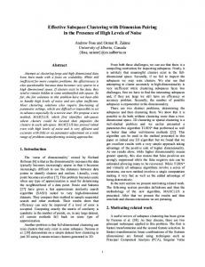
2.4 Model-Based Clustering Model-based clustering (MBC) [5, 11] is a parametric statistical approach that assumes: the data X = {x1 , x2 , ..., xn }, xi ∈ RK are an independently and identically distributed sample from an unknown population density p(x); each population group g is represented by a (often Gaussian) density pg (x); and p(x) is a weighted mixture of these density components, P P i.e. p(x) = Gg=1 πg · pg (x; θg) where πg = 1, 0 < πg ≤ 1 for g = 1, 2, ..., G, and θg = (µg , Σg ) for Gaussian components. The method chooses the number of components G by maximizing the Bayesian Information Criterion (BIC) and estimates the means and variances (µg , Σg ) via maximum likelihood. While it may assume Gaussian components, its flexibility on their shape, volume, and orientation allows student groups of varying shapes and sizes. MBC also often fits overlapping components in an effort to improve fit; users are not able to specify cluster separation information and are also required to give a range of possible numbers of clusters. If multiple students map to the same hypercube location, MBC may overfit the data by using spikes with near singular covariance in these locations. To alleviate this concern (and improve visualization), we jitter the Bi a small amount (0.01). The effect on our results is minimal. In all three cases, the algorithm returns a set of cluster centers and an assignment vector mapping each Bi to a cluster. A cluster center represents the skill set profile for that subset of students. Note that cluster centers are not restricted to be in the neighborhood of a hypercube corner (although they could be assigned to one). Returning cluster centers rather than their closest corners gives more conservative estimates of skill mastery (vs. 0/1). As a small illustrative example, we use a subset of 26 items requiring three skills from the Assistment System online mathematics tutor [7]. The Q-matrix is unbalanced; Skill 1 (Evaluating Functions) appears in eight items (six single, two triple), Skill 2 (Multiplication) in 20 items (18 single, two triple), and Skill 3 (Unit Conversion) in two items (both triple). Overall, 551 students answered at least one item. Figure 1 shows the corresponding 3-D cube, each corner one of eight true skill set profiles. Since Unit Conversion appears in only two items, BiUC ∈ {0, 12 , 1}; students are mapped to three well-separated planes. 7 7 7 7 7 8888 88 8 8 7 8

1.0

1.0

0.2

0.4

0.6

Evaluate Functions

0.8

1.0

0.8

5

0.0

0.2

0.4

0.6

Evaluate Functions

0.8

1.0

312 9 4 1.0 12 6 6 1011 310 10 10 444 12126 666666 3312 12 12 22222 3 333310 1010 12 10 10 444440.8 12 66 2222 12 12 14 2 10 12 2 14 1 10 12 6 10 14 1 12 0.6 1310 10 13 12 111 10 14 11 0.4 1 13 13 13 1414 1010 11 0.2 1 13 13 14 0.0 1 0.0

0.2

0.4

0.6

0.8

1.0

Evaluate Functions

Figure 1: Cluster Assignments: a) HC, Complete G=8; b) K-means G=8; c) MBC G=14

Multiplication

0.6

Unit Conversion

0.4 0.2 0.0

33 3 7 1.0 1 7 4 777 64444 6 333131133333313311111111 11111111 777770.8 6666 1 1111 11111 1 1 6 7 6 7 6 7 0.6 1 11 1 1 666 86 7 2 0.4 8 77 2 2 88 22 0.2 8 8 2 2 2 0.0

Multiplication

0.6

Unit Conversion

0.4 0.2 0.0

Multiplication

0.4 0.2

Unit Conversion

0.6

0.0

55 5 55 5 5555555 55 555 5

2

33 3 3 4 1.0 4 4 444 33333 3 3333333333333344444433 44444444 444440.8 3 3333 33444 4 4 3333 3 4 3 4 4 2 0.6 3 33 3 3 222 3 6 22 0.4 2 5 5 66 55 12 0.2 1 5 5 6 0.0 1

7 7 7 7 7 7777 78 7 7 7 7

7 7

33 5 55 5 5555555 55 555 5

0.8

0.8

77 7 77 7 7777777 88 888 7 2

0.0

5 5 5 5 5 5555 55 5 5 5 5

5 5

1.0

7 7

Figures 1a-c) show the clusters found by HC (complete), k-means, and MBC respectively. We set G=2K =8 for both HC and k-means; MBC searched over G=1 to 25, choosing 14. Only MBC separated the students in the three Unit Conversion planes (BiUC =0:1-4, 6, 914; BiUC =0.5: 5; BiUC =1: 7, 8). Both HC and k-means combined students with (arguably very) different Unit Conversion capability across planes into clusters. In contrast, MBC assigns one cluster to the students with BiUC =0.5 and two clusters to those with BiUC =1.0 (the corner cluster contains multiple students). In all three solutions, the BiUC =0 students are split among several clusters defined by their BEF and B M capabilities. In the HC and k-means results, these clusters include one to three students with BiUC =0.5. Updating the clusters with new items, skills, etc requires minimal computational time; for example, MBC required ≈ 21 seconds. Classroom teachers can quickly see the changes in the students’ skill knowledge over time. However, none of the three solutions seems the obvious winner. In addition, the user was only able to dictate the number of clusters (and somewhat restrict shape); no guarantees were made about their separation and size.

3 Conditional Subspace Clustering or “Valley-Hunting” In general, clusters are chosen according to a criterion or measure of closeness. Often the user has to define the number of clusters in advance which could be useful to a teacher with fixed resources. For example, he/she might ask for three groups of students clustered on their skill knowledge. However, three clusters may not represent the class well. There may be more or fewer unique skill set profiles. Moreover, the three clusters might be very similar or very different sizes (which both may be impractical). A more useful definition of a cluster might be a well-separated group of students larger than some size threshold. While any skill’s marginal distribution will always have a finite number of unique values, the marginal distribution of some skills may show very well-separated groups of students. We can take advantage of these skills by partitioning the hypercube along their marginal separations. This subsetting alone may be enough to divide students into appropriate clusters. However, it may be the case that there is multivariate cluster structure not detectable by examining the marginal distributions. As such, we advocate using this algorithm either alone or as a dimension reduction tool for other clustering methods. That is, we could first use the marginal distributions to select skills with obvious group structure and then cluster (if needed) the resulting subspaces. Reducing the dimensionality prior to clustering can greatly improve efficiency and/or results [11]. While the Figure 1 hyperplane separation is clear, it could be very difficult to identify obvious separations in a higher dimensional hypercube with noisier marginal distributions. A method to automatically find candidate skills for partitioning (and alert teachers to skills that separate the class) is more desirable. Akin to the nonparametric clustering notion that a density’s mode corresponds to a group in the population [6] and the discretization of continuous variables, we condition on a skill if its marginal distribution contains one or more “significant valleys”, a non-trivial area of low density between two high density areas. This decision is made by investigating the marginal distribution’s contours. Scanning from zero to one, the low density area must be

preceded by a descent and followed by an ascent, both of gradient larger than a specified depth threshold (cluster size), and must be wider than a specified width threshold (cluster separation). There are at least two ways in which low density areas might occur. A skill only occurs in a few items and so has few possible Bik values, or the Bik might be centered around only a few values. If one or more significant valleys are found, we partition the hypercube at the minimum density point of each significant valley. (Other choices could be made, e.g. the halfway point between the two peaks.) In practice, we initially search for significant valleys in all skills’ marginal distributions to select skills for partitioning (if any). The resulting subspaces consisting of dimensions (skills) without obvious separations are then clustered if desired; the results can be combined into one final clustering solution. Let τd , τw be the respective depth and width separation thresholds (user-specified). These thresholds can be constant or differ over skills (τdk , τwk ). For computational ease, we use histograms to represent each skill’s marginal distribution. The user may also choose a histogram bin width. The automatic subspace partitioning algorithm is as follows: For each skill k: Calculate the probability histogram for the given bin width. Let λi = height of Bin i. Define the gradient γi,i+1 as the difference in the percent of students in bins i, i + 1. Let γN = λi − λ j be the total descent gradient from a peak (Bin i) to a valley (Bin j). Let γP = λi − λ j be the total ascent gradient from a valley (Bin i) to a peak (Bin j). Let Lm be the location of the mode preceding the current valley (scan’s startpoint). Let Lv be the location of the lowest height of the current valley. Initialize Lm = Lv = Bin 1. 1) Scan γi,i+1 until γi,i+1 < 0. If no such gradient exists, there are no remaining valleys. 2) Else, scan γi,i+1 until γi,i+1 ≥ 0 (end of valley) or out of bins; compute γN . If |γN | > τd , have found a “significant” descent. Set Lv = Bin i + 1. 3) Scan γi,i+1 until γi,i+1 < 0 (end of peak) or out of bins; compute γP . If |γP | > τd , we have found a “significant” ascent. Find valley width w. If w > τw , significant valley; store mode locations. Else, do not store. In either case, set Lm = Lv = Bin i + 1. Scan for next valley (return to 1). Else, have not found significant ascent. Scan γi,i+1 until γi,i+1 ≥ 0 (end of next valley) or out of bins. If λi+1 < λLv , current valley is lower than valley at Lv . Set Lv = Bin i + 1. (return to 3) Else, current valley is higher than valley at Lv ; have “hiccup mode”. (return to 3) Else, have not found a significant descent. Scan γi,i+1 until γi,i+1 < 0 (end of next peak) or out of bins. If λi+1 > λLm , current peak is higher than peak at Lm . Set Lm = Bin i + 1. Scan for next valley (return to 1). Else, current peak is lower than peak at Lm ; have “hiccup mode”. (return to 2)

Evaluating Functions

Multiplication

Unit Conversion

4

Density

3 2

Density

1.5

Density

1.0

1.0

0.0

0.2

0.4

0.6

B−matrix values

0.8

1.0

0.0

0.2

0.4

0.6

B−matrix values

0.8

1.0

0

0

0.0

0.0

0.5

1

2

0.5

Density

2.0

6

2.5

4

1.5

8

3.0

5

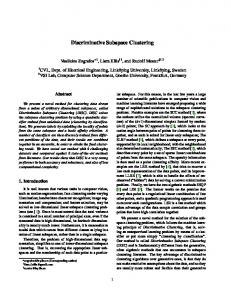
Marginal Distribution of skill k

0.0

0.2

0.4

0.6

B−matrix values

0.8

1.0

0.0

0.2

0.4

0.6

0.8

1.0

B−matrix values

Figure 2: Marginal Skill Distributions: Illustrative Example, Three Assistment Skills

The spirit of our algorithm is similar to mode-hunting (e.g. [12]) excepting that we only want to identify modes that are separated by a valley of substantial depth and width. In a sense, we are “valley-hunting”. For example, if while searching for a descent of substantial depth we find a “hiccup mode” where the marginal distribution slightly increases and then continues to decrease, the algorithm does not view that small valley to be important. (A “hiccup mode” might similarly be found when searching for a substantial ascent.) Figure 2a contains an example marginal distribution of Skill k, a histogram with bin width = 0.10. For example, say a teacher will only adapt classroom strategies for groups of students who are at least 10% of the class and whose capability values are separated by at least 20%. Given τd = 0.1, τw = 0.2, we start at Bin 1 and immediately find a descent of 0.14 (1.5 · 0.10 − 0.1 · 0.10). We know that there is at least one bin in the preceding mode with at least 10% of the students (our depth threshold). We continue scanning to find a total ascent of 0.135 (1.45 · 0.10 − 0.1 · 0.10) at Bin 4, evidence that the next mode also has at least 10% of the students. As both gradients exceed τd , we check that the valley is wide enough by measuring the distance between the two modes (0.0, 0.3). Since 0.3 > 0.2 = τw , both modes are separated by at least 20% capability, and we have identified a “significant valley”. Continuing to scan, we find another descent and valley at Bin 6. In this case, the descent is not large enough yet to indicate a well-separated group (Bin 7 is a “hiccup mode”). A large enough descent is eventually found between Bin 4 and Bin 8, followed by a significant ascent. The next significant valley is then from Bin 4 to Bin 10. We partition the skill at Bin 2 (0.15) and Bin 8 (0.75) to create three groups of students of size at least 10% of the class separated by at least 20% capability on Skill k. If our thresholds were τd = .045, τw = 0.10, four groups would have been found (cutpoints: 0.15, 0.55, 0.75). Figure 2 also includes the three Assistment skill marginal distributions. While Unit Conversion (Figure 2d) has three well-separated peaks, given reasonable depth/size thresholds, our algorithm would not partition this skill since two non-zero bin counts are very small (i.e. modes of trivial mass). We also would likely not partition the skewed Multiplication distribution. Given τd =0.1, τw =0.2, we do partition Evaluate Functions at 0.15, 0.75 for three groups of students and cluster the three subsequent two-dimensional subspaces. Figure 3 shows the methods’ respective results. There is less cross-plane clustering in HC and k-means without partitioning Unit Conversion (Figures 3a,b). MBC again chose 14 total with similar results; however, the subspace clustering (including both finding the partitions and clustering the subspaces) took ≈ 6 seconds (vs. 21) for computational savings of 71%.

7 7 7 7 7 777777 33363633 7 7 3

1.0

1.0

0.2

0.6

Evaluate Functions

0.8

3 0.0

1.0

1

0.2

55

0.4

5

0.6

0.8

3 0.0

1.0

Evaluate Functions

0.8

20.022

2

13 131.0 7777 7 7777 7 7 13333 6 777 13 13 13 111111111 6 66666666666666666666666666666 666666 6 113 313 13 13 0.8 13 13 11111111 13 66444444666 444646 4 6 13 212111 13 13 0.6 22 4 2 2 4 2 4 2 44 4 10 2 22 4 10100.4 4 4 44 4 0.2 22 2 0.2

55

0.4

5

0.6

0.8

Multiplication

0.6

Unit Conversion

0.4 0.2

Multiplication

0.6

Unit Conversion

0.4 0.2

10.011

22 12 11 11 121.0 66666 611 666 1111 11 6666666666666 11611 12 12 11 22222222222 6611 12 10 11 812 10 11 11 10 11 10 10 11 6 6611 11 11 11 11 10 10 1111 10 11 11 11 6 6611 10 11 888880.8 11 10 11 11 11 11 11 10 11 1111 910 80.68 11 11 11 8 11 99 5 9 9 11 9 5 9 55 5 3 9 99 5 3 3 0.4 5 5 55 5 0.2 11 1

0.0

12 0.4 12 12

0.0

4

Multiplication

0.6 0.4

Unit Conversion

0.2

490.0414

9 99 9 9999 9999 99 99 911 9 5

5

11 11 11 111111 10 8338 1.0 11 11 11 4914944 111111 11 11 11 11 44 11 1111 11 11 11 11 11 11 11 11 11 11 444414949914941 11 11 11 11 11 11 383383683 11 11 11 11 1111 11 11 11 11 11 11 11 14494410 094114 1111 11 11 11 333860.8 11 11 11 11 11 11 11 11 11 11 1111 4444914 11 11 30.636 11 11 11 3 11 4 4 11 4 14 11 1111 3 4 44 12 3 2 0.4 12 12 12 1212 0.2 44 4

12 12 8 8 8 8 8 888888 1212 12 12 8 8 12

8 8

77 7 7777 7777 77 77 774 7

0.8

0.8

55 5 5555 5555 55 55 553 5 5

0.0

7 7 7 7 7 777777 444444 7 7 4

7 7

1.0

7 7

140.0 1.0

Evaluate Functions

Figure 3: Cluster Assignments: a) HC, Complete G=3 · 22 ; b) K-means G=3 · 22 ; c) MBC G=14

4 Recovering the True Skill Set Profiles In this section, we simulate data from the DINA model, a common educational research model, to compare the methods’ ability to recover the students’ true skill set profiles. The deterministic inputs, noisy “and” gate model (DINA) is a conjunctive cognitive diagnosis model used to estimate student skill knowledge [10]. The DINA model item response 1−η form is P(yi j = 1 | ηi j , s j , g j )= (1 − s j )ηi j g j i j where αik = I{Student i has skill k} and ηi j = QK q jk k=1 αik indicates if student i has all skills needed for item j; s j = P(yi j =0 | ηi j =1) is the slip parameter; and g j = P(yi j =1 | ηi j =0) is the guess parameter. If student i is missing any of the required skills for item j, P(yi j = 1) decreases due to the conjunctive assumption. Prior to simulating the yi j , we fix the skills to be of equal medium difficulty with an inter-skill correlation of either 0 or 0.25 and generate true skill set profiles Ci for each student. In our work thus far, only a perfect inter-skill correlation has a non-negligible effect on the results. These parameter choices evenly spread students among the 2K natural skill set profiles. We randomly draw our slip and guess parameters (s j ∼ Unif(0,0.30); g j ∼ Unif(0,0.15)). Given the true skill set profiles and slip/guess parameters, we generate the student response matrix Y. Then, using a fixed Q matrix, we calculate and cluster the corresponding B matrix. For the first three methods, no partitioning is done (HC, k-means: G = 2K ; MBC: searches from 1 to G > 2K ). In conditional subspace clustering, we initially use τd = 0.1, τw = 0.2 and then cluster the resulting subspaces (if any). To gauge performance, we calculate their agreement to the true profiles using the Adjusted Rand Index (ARI), a common measure of agreement between two partitions [9]. Under random partitioning, E[ARI] = 0, and the maximum value is one. Larger values indicate better agreement. Table 1 presents selected simulations for K = 3, 7, 10 for varying J, N. In the Cond (MBC) column, the first ARI corresponds to the partitioning alone, the second to the clustering of the partitioned subspaces (with MBC). We also vary the Q-matrix design to include only single skill items, only multiple skill items, or both. In addition, the Q-matrix was balanced (bal) or unbalanced (unbal). If balanced, all skills and skill combinations occur the same number of times. Unbalanced refers to uneven representation of or missing skills (miss).

Table 1: Comparing Clustering Methods with the True Generating Skill Set Profiles via ARIs K 3 3 3 3 3 3 3 7 7 10

J 30 30 30 30 30 30 30 40 40 100

N 250 250 250 250 250 250 250 300 300 2500

Q Matrix Design Single Both, bal Both, unbal, uneven Both, unbal, miss Multiple, bal Multiple, unbal, uneven Multiple, unbal, miss Single Both, unbal, miss Single

HAC 1.000 0.792 0.541 0.582 0.414 0.350 0.235 0.746 0.333 0.876

K-means 1.000 0.615 0.625 0.578 0.419 0.504 0.242 0.553 0.308 0.786

MBC 0.970 0.939 0.703 0.707 0.416 0.515 0.194 0.987 0.386 0.062

Cond (MBC) 1.000 0.531 (0.402) 0.241 (0.641) 0.249 (0.713) 0.222 (0.495) — — 0.982 0.290 0.958

Selected Skills 3 2 1 1 1 0 0 7 3 10

Excepting the multiple unbalanced design, the subspace algorithm selected one or more skills for partitioning (in some cases, all skills were correctly selected). In almost all simulations, MBC was comparable to or better than HC and k-means for true skill set profile recovery. The partitioning method coupled with using MBC on the reduced subspaces gave comparable or better results in all cases except the balanced single and multiple skill design. In addition, subspace partitioning/MBC was always faster than MBC alone. Table 2: Comparison of Depth, Width Thresholds τd 0.1 0.1 0.05 0.05 0.025

τw 0.2 0.1 0.2 0.1 0.1

Cond (MBC) 0.249 (0.713) 0.249 (0.713) 0.569 (0.510) 0.569 (0.510) 0.629 (0.694)

Selected Skills 1 1 2 2 3

In addition, for the fourth K= 3, J= 30 Q matrix design, we vary the depth and width thresholds. Smaller values of τd , τw will find narrower, shallower separations; in addition, smaller isolated clusters will be found. In this particular example, we found that as we decreased the depth threshold, more skills were (correctly) selected, and the performance of the partitioning by itself improved. While the parameters are designed to be user-specified, we are currently exploring their behavior in order to make good default suggestions.

5 Thirteen Skill Assistment Example Finally, we briefly look at a higher dimensional Assistment example with K=13 skills, N=344 students, and J=135 items. This data set included multiple skill items and a large amount of missing response data. HC and k-means are not appropriate choices; finding 213 =8192 clusters is unreasonable (without, say, allowing for empty clusters as in [1]); MBC will largely depend on choosing an appropriate search range. The conditional subspace clustering algorithm, however, searches the space for obvious separation and partitions 9 of the 13 skills for a total of 221 subspaces (1 sec). All subspaces contained ≤ 13 students and so could likely be used alone or as subspaces for further clustering if needed.

6 Conclusions We presented a conditional subspace clustering algorithm for use with the capability matrix (or similar skill knowledge estimate). The method selects skills that separate students well and reduces dimensionality for subsequent clustering. Our work so far shows that for most Q-matrix designs, the recovery of true skill set profiles is comparable or better than other clustering methods while also including skill selection. Since the true profiles in the Assistment examples are unknown, we cannot judge their recovery. However, visual inspection indicates that the partitions and skill selection seem sensible. To our knowledge, work in this area has not adequately addressed the need to analyze high-dimensional Q-matrices. The approach presented, while allowing for real time estimation of student skill set profiles, can handle large numbers of skills as well as incorporate practical user specifications.

References [1] Ayers, E, Nugent, R, Dean, N. “Skill Set Profile Clustering Based on Student Capability Vectors Computed from Online Tutoring Data”. Educational Data Mining 2008: 1st International Conference on Educational Data Mining, Proceedings (refereed). R.S.J.d. Baker, T. Barnes, and J.E. Beck (Eds), Montreal, Quebec, Canada, June 20-21, 2008. p.210-217. [2] Ayers, E, Nugent, R, Dean, N. “A Comparison of Student Skill Knowledge Estimates”. Educational Data Mining 2009: 2nd International Conference on Educational Data Mining, accepted. [3] Barnes, T.M. (2003). The Q-matrix Method of Fault-tolerant Teaching in Knowledge Assessment and Data Mining. Ph.D. Dissertation, Department of Computer Science, NCSU. [4] Chiu, C (2008). Cluster Analysis for Cognitive Diagnosis: Theory and Applications. Ph. D. Dissertation, Educational Psychology, University of Illinois at Urbana Champaign. [5] Fraley, C. and Raftery, A. Mclust: Software for model-based cluster analysis. Journal of Classification, 1999, 16, 297-306. [6] Hartigan, J.A. Clustering Algorithms. Wiley. 1975. [7] Heffernan, N.T., Koedinger, K.R. and Junker, B.W. Using Web-Based Cognitive Assessment Systems for Predicting Student Performance on State Exams. Research proposal to the Institute of Educational Statistics, US Department of Education. Department of Computer Science at Worcester Polytechnic Institute, Worcester County, Massachusetts, 2001. [8] Henson, J., Templin, R., and Douglas, J. Using efficient model based sum-scores for conducting skill diagnoses. Journal of Education Measurement, 2007, 44, 361-376. [9] Hubert, L. and Arabie, P. Comparing partitions. Journal of Classification, 1985, 2, 193-218. [10] Junker, B.W., Sijtsma K. Cognitive Assessment Models with Few Assumptions and Connections with Nonparametric Item Response Theory. Applied Psych Measurement, 2001, 25, 258-272. [11] Raftery, A and Dean, N. Variable Selection for Model-Based Clustering. Journal of the American Statistical Association, Vol. 101, No. 473 (March 2006), pp. 168-178. [12] Silverman, B. W. (1981) Using kernel density estimates to investigate multimodality.J. Royal. Statistical Society Series B. 43: 97-99. [13] Tatsuoka, K.K. (1983). Rule Space: An Approach for Dealing with Misconceptions Based on Item Response Theory. Journal of Educational Measurement. 1983, Vol. 20, No. 4, 345-354.