clustering and video shot detection are also performed. Through the ...... based face clustering by GPCA (a-b), or Mixture of PPCA (c-d), or our algorithm (e-f).
Combined Central and Subspace Clustering on Computer Vision Applications
Le Lu Johns Hopkins University, Baltimore, MD 21218, USA
LELU @ CS . JHU . EDU
Ren´e Vidal Johns Hopkins University, Baltimore, MD 21218, USA
RVIDAL @ CIS . JHU . EDU
Abstract Central and subspace clustering methods are at the core of many segmentation problems in computer vision. However, both methods fail to give the correct segmentation in many practical scenarios, e.g., when data are close to the intersection of subspaces or when two cluster centers in different subspaces are spatially close. In this paper, we address these challenges by considering the problem of clustering a set of points lying in a union of n subspaces and distributed around m cluster centers inside each subspace. We proposed a natural generalization of Kmeans and Ksubspaces by combining central and subspace clustering into the same cost function. It results in an algorithm with easy implementation. Experiments on synthetic data compare our method favorably against four other methods. The validation of our method is also demonstrated with real computer vision problems such as face clustering with varying illumination and video shot segmentation of dynamic scenes.
1. Introduction Many problems in computer vision require the efficient and effective organization of huge-dimensional visual data for information retrieval purposes. Unsupervised learning, mostly clustering, provides a possible way to handle these challenges. Central and subspace clustering are arguably the most studied clustering problems. In central clustering, data samples are assumed to be distributed around a collection of cluster centers, e.g., a mixture of Gaussians. This problem shows up in many vision tasks, e.g., image segmentation, and can be solved using techniques such as Kmeans (Duda Appearing in Proceedings of the 23 rd International Conference on Machine Learning, Pittsburgh, PA, 2006. Copyright 2006 by the author(s)/owner(s).
et al., 2000), Expectation Maximization (EM) (Dempster et al., 1977). In subspace clustering, data samples are assumed to be distributed in a collection of subspaces. This problem shows up in various vision applications, such as motion segmentation (Kanatani, 2003; Vidal & Ma, 2004), face clustering with varying illumination (Ho et al., 2003; Vidal et al., a), image and video segmentation (Vidal et al., a), etc. Subspace clustering can also be used to obtain a piecewise linear approximation of a manifold (Weinberger & Saul, 2004), as we will demonstrate in our real data experiments.Existing subspace clustering methods include Ksubspaces (Ho et al., 2003) and Generalized Principal Component Analysis (GPCA) (Vidal et al., b; Vidal et al., a), which make no assumption about the distribution of the data inside the subspaces. Methods such as Mixtures of Probabilistic PCA (MPPCA) (Tipping & Bishop, 1999) further assume that the distribution of the data inside each subspace is Gaussian and use EM to learn the parameters of the mixture model. Unfortunately, there are many applications in which neither central nor subspace clustering individually are appropriate1 . To illustrate this argument, we first show two toy examples: subspace clustering fails when the data set contains points close to the intersection of two subspaces, as shown in Figure 1. Similarly, central clustering fails when two clusters in different subspaces are spatially close, as shown in Figure 2. Figure 1 and 2 are better visualized in color. Paper contributions. In this paper, we propose a new clustering approach that combines both central and sub1 In motion segmentation, for example, there are two motion subspaces where each of them contains two moving objects and two objects from different motion subspaces are spatially close during moving. If one is interested in grouping based on motion only, one may argue that the problem can be solved by subspace clustering of motion subspace alone. However, if one is interested in grouping the individual objects, the problem can not be well solved using central clustering of spatial locations alone, because the two spatially close objects under different subspaces can confuse central clustering. In this case, some kind of combination of central and subspace clustering should be considered.
Combined Central and Subspace Clustering on Computer Vision Applications
space clustering. We obtain an initial solution by grouping the data into multiple subspaces using GPCA and grouping the data inside each subspace using Kmeans. This initial solution is then refined by minimizing an objective function composed of both central and subspace distances. This combined optimization leads to improved performance of our method over five different clustering approaches in terms of both clustering error and estimation accuracy. Real examples on illumination-invariant face clustering and video shot detection are also performed. Through the visualization of real video data in their feature space, we find that data samples in R3 are usually distributed on complex shaped curves or manifolds, as shown in Figure 8 and 7. With encouraging clustering results, our experiments also validate that subspace clustering can be effectively used to obtain a piecewise linear approximation of complex manifolds. Data map in ℜ3 for Toy Problem 1
Central clustering by GPCA−Kmeans for Toy Problem 1
Subspace clustering by GPCA for Toy Problem 1
10
10
10
8
8
8 6
6
6
A1
Z 4
A1
A1 Z 4
2
B2
0
Z
B2
0
B1
B1
B1
5 10
Y
−2 −10
Y 0
Y 0 10
5
0
−5
−10
10
−5
−10
X
10
10
5
0
X
10
5
0
−5
−10
X
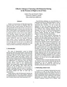
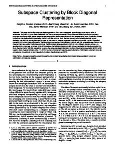
Figure 1. Left: A set of points drawn from the x-y plane and the y-z plane, and distributed around two cluster centers inside each plane which are labelled as A1 , A2 B1 , B2 respectively. Note that some data points are drawn from the intersection of the two planes (ie. y-axis). Center: Subspace clustering by GPCA incorrectly assigns all the points on the y-axis to the y-z plane. Right: Central clustering by applying Kmeans to the two groups given by GPCA incorrectly assigns points in B2 to A1 . Data map in ℜ3 for Toy Problem 2
Central clustering by GPCA−kmeans for Toy Problem 2
Central clustering by kmeans for Toy Problem 2
A1
9
A1
10
A1
10
8 7
8
8
A2
A2
6
A2 6
6
5
Z
Z
4
Z 4
4
3
B1
2
2
2
B1
B1
1 −10
B2
0
0 −1 −4
−2
0
2
4
6
X
8
10
10
0
−10 0 Y
B2
Y −2 −4
P
m
. XX JKM = wik kxi − µk k2 .
(1)
i=1 k=1
Given the cluster centers, the optimal solution for the memberships is to assign each point to the closest center. Given the memberships, the optimal solution for the cluster centers is given by the means of the points within each group. The Kmeans algorithm proceeds by alternating between these two steps until convergence to a local minimum.
B2
A2
0
A2
−2 −10
0
Note that when n = 1 Problem 1 reduces to the standard central clustering problem. A popular method for solving this problem is the Kmeans algorithm, which solves for the cluster centers µk and the membership of the i-th point to the k-th cluster center, wik ∈ {0, 1}, by minimizing the within class variance
2
2
A2 −2 −5
4
normal bases {Bj ∈ R(D−dj )×D }nj=1 . Assume that within each subspace Sj the data points are distributed around m k=1...m cluster centers {µjk ∈ RD }j=1...n . Given {xi }P i=1 , estin k=1...m mate {Bj }j=1 and {µjk }j=1...n .
−2
0
2
X
4
6
8
10
10
0
−10
B2 −2 −4
−2
0
2
X 4
6
8
0 Y 10
10
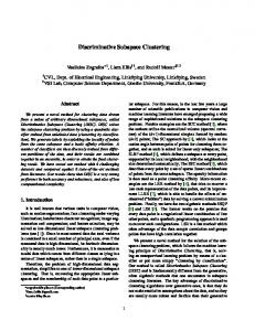
Figure 2. Left: A set of points drawn from the x-y plane and the y-z plane, and distributed around two cluster centers inside each plane which are labelled as A1 , A2 B1 , B2 respectively.. Note that one of the blue clusters (B2 ) is spatially close to one of the red clusters (A2 ). Center: Central clustering by Kmeans assigns some points in A2 to B2 . Right: Subspace clustering using GPCA followed by central clustering inside each subspace using Kmeans gives the correct clustering into four groups.
2. Combined Central and Subspace Clustering In this paper, we consider the following problem. Problem 1: Let {xi ∈ RD }P i=1 be a collection of points lying approximately in n subspaces Sj = {x : Bj> x = 0} with
Note also that when m = 1 Problem 1 reduces to the classical subspace clustering problem. As shown in (Ho et al., 2003), this problem can be solved with an extension of Kmeans, called Ksubspaces, which solves for the subspace normal bases Bj and the membership of the i-th point to the j-th subspace, wij ∈ {0, 1}, by minimizing the cost function P
n
. XX JKS = wij kBj> xi k2
(2)
i=1 j=1
subject to the constraints Bj> Bj = I, for j = 1, . . . , n, where I denotes the identity matrix. Given the normal bases, the optimal solution for the memberships is to assign each point to the closest subspace. Given the memberships, the optimal solution for the normal bases is obtained from the null space of the data within each group. The Ksubspaces algorithm proceeds by alternating between these two steps until convergence to a local minimum. In this section, we are interested in the more general problem of n > 1 subspaces and m > 1 centers per subspace where it is straightforward to be generalized by having different m for each subspace. In principle, we could also solve this problem using Kmeans by interpreting Problem 1 as a central clustering problem with mn cluster centers. However, Kmeans does not fully employ the data’s structural information and can cause undesirable clustering results, as shown in Figure 2. Thus, we propose a new algorithm which combines the objective functions (1) and (2) into a single objective, and is a natural generalization of both Kmeans and Ksubspaces to simultaneous central and subspace clustering.
Combined Central and Subspace Clustering on Computer Vision Applications
For the sake of simplicity, we further assume that the subspaces are of co-dimension one, i.e. hyperplanes, so that we can represent them with a single normal vector bj ∈ RD . We discuss the extension to subspaces of any dimensions in Remark 2. Our method computes the cluster centers and the subspace normals by solving the following optimization problem min
P X n X m X
³ ´ 2 2 wijk (b> j xi ) + kxi − µjk k (3)
i=1 j=1 k=1
subject to
b> j bj = 1, j = 1, . . . , n b> j µjk = n X m X
(4)
0, j = 1, . . . , n, k = 1, . . . , m (5)
wijk = 1, i = 1, . . . , P
(6)
j=1 k=1
where wijk ∈ {0, 1} denotes the membership of the i-th point to the jk-th cluster center. Equation (3) ensures that for each point xi , there is a (j, k) such that both |b> j xi | and kxi − µjk k are small2 , equation (4) ensures that the normal vectors are of unit norm, equation (5) ensures that each cluster center lies in its corresponding hyperplane, equation (6) ensures that each point is assigned to only one of the mn cluster centers. Using the technique of Lagrange multipliers to minimize the cost function in (3) subject to the constraints (4)–(6) leads to the new objective function P X n X m X 2 2 L= wijk ((b> j xi ) +kxi −µjk k )+ i=1 j=1 k=1 n X m X j=1 k=1
λjk (b> j µjk )+
n X δj (b> j bj −1).
(7)
j=1
Similarly to the Kmeans and Ksubspaces algorithms, we minimize L using the following coordinate descent minimization technique. The following subsections describe each step of the algorithm in detail. Initialization: Since the data lies in a collection of hyperplanes, we can apply GPCA to obtain an estimate of the normal vectors {bj }nj=1 and segment the data into n groups. Let X j ∈ RD×Pj be the set of points in the jth hyperplane. If we use the SVD of X j to compute a rank D − 1 approximation of X j ≈ Uj Sj Vj , where Uj ∈ RD×(D−1) , Sj ∈ R(D−1)×(D−1) and Vj ∈ R(D−1)×Pj , then the columns of X 0j = Sj Vj ∈ R(D−1)×Pj are a set of vectors in RD−1 distributed around m cluster centers. We can apply Kmeans to segment the columns of 2
The other reason to employ the sum of two distances here is to be consistent with the log-likelihood formulation in remark 1.
Algorithm 1 (Combined Central and Subspace Clustering) 1. Initialization: Obtain an initial estimate of the normal veck=1...m tors {bj }n j=1 and cluster centers {µjk }j=1...n using GPCA followed by Kmeans in each subspace. 2. Computing the memberships Given the normal vectors k=1...m {bj }n j=1 and the cluster centers {µjk }j=1...n , compute the memberships {wijk }. 3. Computing the cluster centers: Given the memberships {wijk } and the normal vectors {bj }n j=1 , compute the cluster centers {µjk }k=1...m . j=1...n 4. Computing the normal vectors: Given the memberships {wijk } and the cluster centers {µjk }k=1...m j=1...n , compute the normal vectors {bj }n j=1 . 5. Iterate: Repeat steps 2,3,4 until convergence of the memberships.
X 0j into m groups and obtain the projected cluster centers {µ0jk ∈ RD−1 }m k=1 . The original cluster centers are then given by µjk = Uj µ0jk ∈ RD . Computing the memberships: Since the cost function is always positive and linear in wijk , the minimum is attained P by choosing wijk = 0. However, since jk wijk = 1, the ¡ ¢ 2 2 wijk multiplying the smallest (b> j xi ) + kxi − µjk k must be 1, hence ( ¡ ¢ 2 2 1 if (j, k) = arg min (b> j xi ) + kxi − µjk k wijk = . 0 otherwise (8) Computing the cluster centers: From the first order condition for a minimum we have P X ∂L = −2 wijk (xi − µjk ) + λjk bj = 0. ∂µjk i=1
(9)
> After left-multiplying (9) by b> j and recalling that bj µjk = > 0 and bj bj = 1, we obtain
λjk = 2
P X
wijk (b> j xi ).
(10)
i=1
After substituting (10) into equation (9) and dividing by two, we obtain −
P P X X wijk (xi −µjk ) + wijk bj b> j xi = 0 =⇒ i=1
i=1
PP µjk = (I −
bj b> j )
i=1
PP
wijk xi
i=1
wijk
Combined Central and Subspace Clustering on Computer Vision Applications
where I is the identity matrix in RD . Note that µjk has a simple geometric interpretation: it is the mean of the points in the jk-th cluster, projected onto the j-th hyperplane. Computing the normal vectors: From the first order condition for a minimum we have
and σ −2 = σb−2 − σµ−2 . The optimal solution can be obtained using coordinate descent, similarly to Algorithm 1, as follows λjk = 2
i=1
P X m m X X ∂L =2 wijk (b> λjk µjk + 2δj bj = 0. j xi )xi + ∂bj i=1 k=1
b> j
After left-multiplying (11) by to eliminate λjk and recalling that b> µ = 0, we obtain j jk δj = −
P X m X
2 wijk (b> j xi ) .
(12)
i=1 k=1
After substituting (10) into equation (11) and recalling that b> j µjk = 0, we obtain P X m X ( wijk (xi + µjk )x> i + δj I)bj = 0.
(13)
i=1 k=1
PP Pm Then bj is the eigenvector of ( i=1 k=1 wijk (xi + µjk )x> i + δj I) associated with its smallest eigenvalue, which can be computed using the SVD. Remark 1: Maximum Likelihood Solution
P X n X m X i=1 j=1 k=1
wijk
³ (b> xi )2 j
2σ 2
+
kxi − µjk k2 + log(σb ) 2σµ2
n X m ´ X + (D − 1) log(σu ) + λjk (b> j µjk ) j=1 k=1 n X
δj (b> j bj − 1)
+
j=1 (b> xi )2
kx −µ
k2
where wijk ∝ exp(− j2σ2 − i 2σ2jk ) is now the probµ ability that the i-th point belongs to the jk-th cluster center,
b> j xi σµ2
δj = −
P X m X
P X m X
wijk
i=1 k=1
PP
2 (b> j xi ) σ2
wijk xi
i=1
wijk
xi µjk + δj I)bj + 2 )x> 2 σ σµ i i=1 k=1 PP Pn Pm > 2 i=1 j=1 k=1 wijk (bj xi ) 2 σb = PP Pn Pm wijk i=1 ¢ ¡ j=1 k=1 P > 2 2 w kx − µ k − (b x ) ijk i jk i j ijk σu2 = PP Pn Pm (D − 1) i=1 j=1 k=1 wijk
0=(
wijk (
Remark 2: Extension from hyperplanes to subspaces In the case of subspaces of co-dimension larger than one, each normal vector bj should be replaced by a matrix of normal vectors Bj ∈ RD×(D−dj ) , where dj is the dimension of the j-th subspace. Since the normal bases and the means must satisfy Bj> µjk = 0 and Bj> Bj = I, the objective function (3) should be changed to L=
Notice that in the combined objective function (7) the term |b> j xi | is the distance to the j-th hyperplane, while kxi − µjk k is the distance to the jk-th cluster center. Since the former is mostly related to the variance of the noise in the orthogonal direction to the hyperplane, σb2 , while the latter is mostly related to the within class variance, σµ2 , the magnitudes of these two distances need to be taken into account. One way of doing so is to assume that the data is generated by a mixture of mn Gaussians with means µjk > 2 and covariances Σjk = σb2 bj b> j + σu (I − bj bj ). This automatically allows the variances inside and orthogonal to the hyperplanes to be different. Application of the EM algorithm to this mixture model leads to the minimization of the following normalized objective function
wijk
i=1 µjk = (I − bj b> j ) PP
k=1
(11)
L=
P X
P X n X m X
wijk (kBj> xi k2 + kxi − µjk k2 )+
i=1 j=1 k=1 n X m X
> λ> jk (Bj µjk ) +
j=1 k=1
n X
¡ ¢ trace ∆j (Bj> Bj − I) .
j=1
(14) where λjk ∈ R(D−dj ) and ∆j ∈ R(D−dj )×(D−dj ) are, respectively, vectors and matrices of Lagrange multipliers. Given the normal basis Bj , the optimal solution for the means is given by PP wijk xi > µjk = (I − Bj Bj ) Pi=1 . P i=1 wijk One can show that the optimal solution for ∆j is a scaledPidentity matrix whose diagonal entry is P Pm Given δj and δj = − i=1 j=1 wijk kBj> xi k2 . µjk , Bj can still be solved from the null space of PP Pm ( i=1 k=1 wijk (xi + µjk )x> i + δj I) which can be proved to have dimension D − dj .
3. Experiments 3.1. Comparison of clustering performance with simulated data We randomly generate 600 data points in R3 lying in 2 intersecting planes {Sj }2j=1 with 3 clusters in each plane
Combined Central and Subspace Clustering on Computer Vision Applications
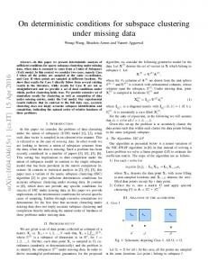
Figure 3 shows a comparison of the performance of the above methods in terms of clustering error ratiosand the error in the estimation of the normal directions in degrees. The results are the mean of the errors over 100 trials. It can be seen in Figure 3 that the errors in clustering and normal vectors of all four algorithms increase as a function of noise. MP achieves better performance than KM and KK for large levels of noise, probably via its probabilistic formulation. The two stage algorithms, KK, GK and JC, in general perform better than KM and MP in terms of clustering error. The random initialization based methods, KM, MP and KK, have non-zero clustering error even with noise-free data. Within the two stage algorithms, KK begins to experience subspace clustering failures more frequently with more severe noises, due to its random initialization, while GPCA in GK and JC employ an algebraic solution of one-shot subspace clustering, thus avoiding the initialization problem. The incorrect subspace clustering of KK can cause the estimate of the normals to be very inaccurate, which explains why KK has worse errors in the normal vectors than KM and MP4 . In summary, GK and JC have smaller average errors in clustering and normal vectors than KM, MP and KK . The combined optimization procedure of JC converges within 2 ∼ 5 iterations according to our experiments, which further advocates JC’s clustering performance. 3
Software available at www.ncrg.aston.ac.uk/netlab/ In order to estimate the plane normals, we group 6 clusters returned by KM or MP into 2 planes. The idea is that 3 clusters which lie in the same plane have`the ´ dimensionality of 2 instead of 3. A brute-force search with 63 /2 selections is employed to find the 2 best fitting planes, by considering the minimal strength of the data distributed in the third dimension via Singular Value Decomposition (Duda et al., 2000). 4
Comparison of clustering errors under different ratios of σ / σ
µ
b
0.09
Kmeans+grouping MPPCA+grouping K−subspace+Kmeans GPCA+Kmeans GPCA+Kmeans+Optimization
0.08
clustering error ratio
0.07 0.06 0.05 0.04 0.03 0.02 0.01 0 0
1
2
4
ratios of σb / σµ %
7
10
Comparison of errors of normal under different ratios of σ / σ b
10 9
errors of normal (degree)
{µjk }k=1,2,3 j=1,2 .100 points are drawn around each one of the six cluster centers according to a Gaussian distribution with σµ = 1.5. The angle between the two planes is randomly chosen from 20o ∼ 90o , and the distance among the three cluster centers is randomly selected in the range 2.5σµ ∼ 5σµ . Gaussian noise with standard deviation σb is added in the direction orthogonal to each plane. Based on the simulated data, we compare 5 different clustering methods: • Kmeans clustering in R3 with 6 cluster centers, then merging into 2 planes (KM), • MPPCA3 clustering using 6 cluster centers, then merging them into 2 planes (MP), • Ksubspaces clustering in R3 , then Kmeans within each plane Sj ; j = 1, 2 (KK), • GPCA clustering in R3 , then Kmeans within each plane Sj ; j = 1, 2 (GK), • GPCA-Kmeans clustering for initialization followed by combined central and subspace clustering (JC) as described in Section 2 (Algorithm 1).
8
µ
Kmeans+grouping MPPCA+grouping K−subspace+Kmeans GPCA+Kmeans GPCA+Kmeans+Optimization
7 6 5 4 3 2 1 0 0
2
4
6
ratios of σ / σ % b
8
10
µ
Figure 3. Left: Clustering error as a function of noise in the data. Right: Error in the estimation of the normal vectors (degrees) as a function of the level of noise in the data.
3.2. Applications with real data 3.2.1. FACE CLUSTERING WITH VARYING ILLUMINATION
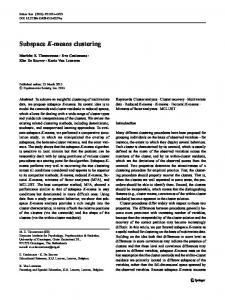
The Yale face database B (Ho et al., 2003) contains a collection of face images Ij ∈ RK of 10 subjects taken under 576 viewing conditions (9 poses × 64 illumination conditions). Here we only consider the illumination variation for face clustering in the case of frontal face images. Thus our task is to sort the images taken for the same person by using our combined central-subspace clustering algorithm. From (Ho et al., 2003), we know that the set of all images of an assumed Lambertian object (such as a human face with a fixed pose) taken under all lighting conditions forms a cone in the image space which can be well approximated by a low dimensional subspace. Thus image sets of different subjects consist of different subspaces. Since the number of pixels K of each image is in general much larger than the dimension of the underlying subspace, PCA (Duda et al., 2000) is first employed for dimensionality reduction. Successful GPCA clustering results have been reported by (Vidal et al., a) for a subset of 3x64 images of subjects 5,8,10. The images in (Vidal et al., a) are cropped as 30x40 pixels and 3 PCA components are used as image features in homogeneous coordinates. In this paper, we further explore the performance of combined centralsubspace face clustering under more complex imaging conditions. We use 4x64 (240x320 pixels) images of subjects 5,6,7,8, which gives more background details (as shown in Figure 4) and keeps 3 PCA components. Figures 5 (a,b) show the imperfect clustering result of GPCA due to the intersection of the subspace of subject 5 with the subspaces
Combined Central and Subspace Clustering on Computer Vision Applications
of subjects 6 and 7. GPCA classifies all the images on the intersections of subspaces into subject 5. Mixtures of PPCA is implemented in Netlab as a probabilistic variation of subspace clustering with one spatial center per subspace. It can be initialized with Kmeans (originally in Netlab) or GPCA, which all result in imperfect clustering outputs. We show one example of the subspaces of subjects 6 and 7 mixed (Kmeans initialization) in Figure 5 (c,d). Our combined subspace-central optimization process successfully corrects the clustering labels of portions of images for subjects 6 and 7, as demonstrated in Figure 5 (e,f). In the optimization, the local clusters in the subspace of subject 6,7 contribute smaller central distances to their misclassified images, which re-classifies them to the correct subspaces using our combined subspace-central clustering algorithm. In this experiment, 4 subspaces with 2 clusters per subspace are used. Compared with the result in (Vidal et al., a), we obtain the perfect illumination-invariant face clustering where data distribution is more complex. 3.2.2. V IDEO SHOT SEGMENTATION Unlike face images under different illumination conditions, video data provides continuous visual signals. Video structure parsing and analysis applications need to segment the whole video sequence into several video shots. Each video shot may contain hundreds of image frames which are either captured with a similar background or have a similar semantical meaning. Figure 6 shows 2 sample videos, mountain.avi and drama.avi, containing 4 shots each. Archives are publicly available from http://www.open-video.org. For the mountain sequence, 4 shots are captured. The shots display different backgrounds and show either multiple dynamic objects and/or severe camera motions. In this video, the frames between each pair of successive shots are gradually blended from one to another5 . In order to explore how the video frames are distributed in feature space, we plot the first 3 PCA components for each frame in Figure 8 (b, d, f). Note that a manifold structure can be observed which starts from red dots to green, black dots and ends in blue (is also listed from shot 1 to shot 4 manually) as shown in Figure 8 (f). The video shot segmentation results of the mountain sequence by Kmeans,GPCA and GPCA-Kmeans followed by combined optimization are shown in Figure 8 (a,b), (c,d) and (e,f), respectively. Because Kmeans is based on the central distances among data, it segments the data into spatially close blobs. There is no guarantee that these spatial blobs will correspond to correct video shots. Comparing Figure 8 (b) with the correct segmentation in (f), the Kmeans algorithm splits shot 2 into clusters 2 and 3, while it groups 5 Due to this reason, the correct video shot segmentation is considered to split every two successive shots at their blending frames.
shots 1 and 4 into cluster 1. By considering the data’s manifold nature, GPCA provides a more effective approximation with multiple planes to the manifold in R3 than the spatial blobs given by central clustering. The essential problem for GPCA is that it only deploys the co-planar condition in R3 , without any constraint relying on their spatial locations. In the structural approximation of the data’s manifold, there are many intersecting data points among 4 planes. These data points represent video frames with the clustering ambiguity solely based on the subspace constraint. Fortunately this limitation can be well tackled by GPCA-Kmeans with combined optimization. Combining central and subspace distances provides correct video shot clustering results for the mountain sequence, as demonstrated in Figure 8 (e,f). The second video sequence shows a drama scenario which is captured with the same background. The video shots should be segmented by the semantic meaning of the performance of the actor and actress. In Figure 6 (Right), we show 2 sample images for each shot. This drama video sequence contains very complex actor and actress’ motions in front of a common background, which results in a more complex manifold data structure6 than that of the mountain video. For better visualization, the normal vectors of data samples recovered by GPCA or the combined central-subspace optimization, are drawn originating from each data point in R3 with different colors for each cluster. For this video, the combined optimization process shows a smoother clustering result in Figure 7 (c,d), compared with (a,b). In summary, GPCA can be considered as an effective way to group data in a manifold into multiple subspaces or planes in R3 which normally better present video shots than central clustering. GPCA-Kmeans with combined optimization can then associate the data at the intersection of planes into the correct clusters by optimizing combined distances. Subspace clustering seems to be a better method to group the data on a manifold by somehow preserving their geometric structure. Central clustering, such as Kmeans7 , provides a piecewise constant approximation; while subspace clustering shows a piecewise linear approximation. On the other hand, subspace clustering can meet severe clustering ambiguity problems when the shape of the manifold is complex, as shown in Figure 7 (b,d). In this case, there are many intersections of subspaces so that subspace clustering results can be very sparse, without considering the spatial coherence. Combined optimization of central and subspace distances demonstrates superior clus6 Because there are image frames of transiting subject motions from one shot to another, the correct video shot segmentation is considered to split successive shots at their transiting frames. 7 Due to space limitation, we do not provide the clustering result using Kmeans for this sequence which is similar with Figure 8 (a,b).
Combined Central and Subspace Clustering on Computer Vision Applications
tering performance with real video sequences.
Figure 4. Sample images of subjects 5,6,7,8.
Data map in ℜ3 for subspace clustering of face data by GPCA−Kmeans
Subspace clustering of face data by GPCA Subject 7
4
0.15 0.1
Class label
Subject 6
0.05
3
0 −0.05
2
Figure 6. Video shot segmentation. Left: Sample images from the mountain sequence. Right: Sample images from the drama sequence.
Subject 5
−0.1 −0.15
Subject 8 0.2
−0.2 −0.1
1
0.1 −0.08
0
50
100
150
200
250
0 −0.06
300
−0.1
−0.04
Image number
−0.02
(a)
−0.2
(b)
Subspace clustering of face data by Mixture of PPCA Data map in ℜ3 for subspace clustering of face data by Mixture of PPCA
4 Subject 7
Class label
0.15
Subject 6
3 0.1 0.05 0
2
Subject 5
−0.05 −0.1
1
0.2
Subject 8
−0.15
0.1
0
50
100
150
200
250
300
−0.2 −0.1
0 −0.09
−0.08
Image number
−0.07
−0.06
−0.1 −0.05
(c)
−0.04
−0.03
−0.2
−0.02
(d)
Subspace clustering of face data by GPCA−kmeans + joint optimization GPCA−Kmeans + joint optimization
4
Subject 7 0.15
Class label
0.1
3
Subject 6
0.05 0 −0.05
2
lection criteria of two types of clustering into one joint or combined process is more difficult than the combination of the clustering algorithms itself, and is under investigation. The examples are toy problem 2 and multiple moving object clustering.The case is more like using additional subspace constraints to balance the central clustering results, which results in a combined distance metric. Secondly, for examples of toy problem 1, face clustering and video segmentation, they are essentially subspace clustering problems and only the number of subspace n turns out to be critical. This case is using (spatial) central distance constraints to solve the inherent ambiguity of subspace clustering at the intersection of any two subspaces. Empirically, m can vary within a moderate range (2 ∼ 5, in our experiments) with similar clustering results8 .
Subject 5
−0.1 −0.15
0.2
Subject 8
1 0
50
100
150
200
250
300
−0.2 −0.1 −0.09 −0.08 −0.07 −0.06 −0.05 −0.04 −0.03 −0.02
0.1 0
−0.2
Image number
(e)
4. Conclusions
−0.1
(f)
Figure 5. According to the correct clustering in (e-f), subjects 5, 6, 7, 8 are grouped as clusters 3, 4, 2, 1 on the left, and shown in with proper labels and color-shapes on the right respectively. Subspace based face clustering by GPCA (a-b), or Mixture of PPCA (c-d), or our algorithm (e-f). The colors of points in this figure also match the colors of subjects 5,6,7,8 in Figure 4.
3.2.3. D ISCUSSION ON M ODEL S ELECTION FOR R EAL DATA We discuss the model selection issue of our algorithm for real data in two cases. Firstly, if strictly following the definition of Problem 1, both the number of subspace n and the number of clusters within each subspace m need to be known beforehand our clustering algorithm. We can employ the model selection algorithms for subspace and central clustering separately in a sequential manner, to determine n first and then m. How to integrate the model se-
In summary, this paper makes three contributions. First, we propose a combined central and subspace clustering algorithm via optimization of a suitable objective function incorporating both types of constraints. It is an intuitive, easy to implement, practically useful and necessary compliment for existing clustering algorithms. Second, the advantage of our algorithm of handling more clustering conditions, compared with traditional Kmeans and Ksubspaces/GPCA methods is illustrated by two toy problems. The comprehensive comparison of four clustering solutions based on 8
If m is too large, the spatial constraints will be too local, which loses the stability of global data structure. For instance, the incorrectly subspace-clustered data samples in (Figure 1 center) can form a separate central based cluster in the y-z plane, and the central constraints from the x-y plane become invalid. If m is too small, the spatial constraints will be too global so that the clustering algorithm can not be adaptive to local structures. Especially for loosely spatially distributed data inside each subspace, the data samples which are too far away should contribute less for the central based constraints to the samples near the subspace intersection.
Combined Central and Subspace Clustering on Computer Vision Applications Shot detection of mountain sequence by kmeans
Shot detection of drama sequence by GPCA
Data Map in ℜ3 shot detection of drama sequence by GPCA
4
4
Shot 1
−0.2
0.05
2
3
2
−0.15
Shot 3
0
Class label
Class label
Shot 4 3
−0.1 −0.05
1
100
200
300
400
500
600
700
800
900
Image frame
−0.1 −0.1
Shot 2
1
−0.05 0
−0.05
0
0.05
(a)
0.1
0.15
0.2
0.25
0
0.05
100
200
300
400
600
700
800
900
(a)
(b)
(b)
Shot detection of mountain sequence by GPCA
Data Map in ℜ3 for shot detection of drama sequence by GPCA−kmeans + joint optimization
Shot detection of drama sequence by GPCA−kmeans + joint optimization
500
Image frame
4 Shot 1
Class label
4
Class label
Shot 4
3
0.08 0.06 0.04
3
2
0.02
2
−0.2
0
Shot 3 −0.02 −0.04
1
−0.15
Shot 2
−0.1
1
−0.06 −0.05 −0.08
200
300
400
500
600
Image frame
(c)
700
800
900
−0.1
0
0
−0.1 −0.05
0
0.05
0.1
0.15
0.2
100
200
300
400
500
600
700
800
900
Image frame
0.05 0.25
(c)
(d)
Figure 7. According to the correct clustering in (c-d), video shots 1, 2, 3, 4 are grouped as clusters 4, 3, 2, 1 on the left, and shown with normal vectors with different directions on the right respectively. Video shot segmentation of drama sequence by GPCA (a-b), or our algorithm (c-d).
(d)
Shot detection of mountain sequence by GPCA−kmeans + joint optimization 4
Shot 3
Class label
100
3
Shot 4 Shot 1
2 Shot 2
1
simulated data demonstrates our algorithm’s priority in accuracy. Third, our method provides an effective and efficient piecewise linear approximation of curved manifolds of complex visual data in video. The video data can be grouped through subspace clustering, while central distance constraints eliminate the clustering ambiguity of subspace intersections. As a future work, we expect to extend the proposed combined central and subspace clustering formulation to recognize multiple complex curved manifolds. An example problem is to find which movie a given images appear in. Each manifold will be composed of multiple subspaces where each subspace is spatially constrained by central distances among data samples. Once the movie models are learned (similarly as shot detection), the likelihood evaluation for a new data sample is based on computing its combined central and subspace distances to the given models.
References Dempster, A., Laird, N., & Rubin, D. (1977). Maximum likelihood from incomplete data via the em algorithm (with discussion). JRSS. Duda, R., Hart, P., & Stork, D. (2000). Pattern classification, 2002. Wiley, New York. 2nd edition. Ho, J., Yang, M.-H., Lim, J., Lee, K.-C., & Kriegman, D. (2003). Clustering apperances of objects under varying illumination conditions. CVPR 2003.
0
100
200
300
400
500
600
700
800
900
Image frame
(e)
(f)
Figure 8. According to the correct clustering in (e-f), video shots 1, 2, 3, 4 are grouped as clusters 1, 2, 4, 3 on the left, and shown in ellipses with proper color-shapes on the right respectively. In (f), three arrows show the topology of the video manifold. Video shot segmentation of mountain sequence by Kmeans (a-b), or GPCA (c-d) or our algorithm (e-f).
Kanatani, K. (2003). Motion segmentation by subspace separation and model selection. ICCV 2001. Tipping, M., & Bishop, C. (1999). Mixtures of probabilistic principal component analyzers. Neural Computation. Vidal, R., & Ma, Y. (2004). A unified algebraic approach to 2-D and 3-D motion segmentation. ECCV 2004. Vidal, R., Ma, Y., & Piazzi, J. A new GPCA algorithm for clustering subspaces by fitting, differentiating and dividing polynomials. CVPR 2004. Vidal, R., Ma, Y., & Sastry, S. Generalized Principal Component Analysis (GPCA). CVPR 2003. Weinberger, K., & Saul, L. (2004). Unsupervised learning of image manifolds by semidefinite programming. CVPR 2004.