Effects of Random Sampling on SVM Hyper-parameter Tuning Tom´ aˇs Horv´ ath1? , Rafael G. Mantovani2 , and Andr´e C. P. L. F. de Carvalho2 1
2
Faculty of Informatics, E¨ otv¨ os Lor´ and University Budapest, Hungary
[email protected] Institute of Mathematical and Computer Sciences, University of S˜ ao Paulo S˜ ao Carlos, Brazil {rgmantov,andre}@icmc.usp.br
Abstract. Hyper-parameter tuning in use is one of the crucial steps in the application of machine learning algorithms. In general, the tuning process is modeled as an optimization problem for which several methods have been proposed. For complex algorithms, the evaluation of a hyper-parameter configuration is expensive and their runtime is sped up through data sampling. In this paper, the effect of sample sizes to the results of hyper-parameter tuning process is investigated. Hyperparameters of Support Vector Machines are tuned on samples of different sizes generated from a dataset. Hausdorff distance is proposed for computing the differences between the results of hyper-parameter tuning on two samples of different size. 100 real-world datasets and two tuning methods (Random Search and Particle Swarm Optimization) are used in the experiments revealing some interesting relations between sample sizes and results of hyper-parameter tuning which open some promising directions for future investigation in this direction. Keywords: Sampling, Hyper-parameter tuning, Suport Vector Machines
1
Introduction
Hyper-parameter (HP) tuning of Machine Learning (ML) algorithms is a challenging task because of some practical difficulties: First, good hyper-parameter (HP) settings depend on the dataset used, so the HP tuning should take into account the algorithm-dataset combination. Second, the individual HP values in good HP settings are often related to each other, thus, independent tuning of individual HP values should be avoided. Finally, evaluating the fitness of a specific HP setting can be computationally expensive, an issue on which this paper is focused on. The choice of the most adequate technique for HP tuning approach depends on the complexity of the ML algorithm used w.r.t. the given data, i.e. if the ?
Tom´ aˇs Horv´ ath is also a member of the Institute of Computer Science, Faculty of ˇ arik University in Koˇsice, Slovakia. Science, Pavol Jozef Saf´
2
T. Horv´ ath et al.
evaluation of the HP setting for a ML algorithm has a low or high computational cost. In other words, if many different HP settings can be easily evaluated or HP have to be tuned from a small number of evaluations. An alternative to speed up the runtime of ML algorithms is sampling [5], when a reduced but representative sample of the data is used to induce a model, instead of using the whole dataset. In addition to random sampling [13], there are more sophisticated (stratified) sampling methods [9, 19] which can be used. The motivation behind the research presented in this paper lies in the following question: In what extent does sampling of a dataset affect the results of HP tuning? A preliminary research, an experiment, was conducted in order to investigate the previous question. Experiments were conducted on 100 real-world datasets and two tuning techniques for HP tuning pf Support Vector Machines (SVM). For comparing the results of HP tuning on different sample sizes, the use of the Hausdorff distance was proposed. Experiments reveal interesting relations which serve as the basis for the further research in this direction.
2
Hyper-parameter Tuning
HP tuning is, in general, treated as an optimization problem whose objective function f : A × D × H → R captures the predictive performance of an algorithm a ∈ A with the HP setting h = (h1 , h2 , . . . , hk ) ∈ H on the dataset D ∈ D where A is the set of ML algorithms, D is the set of datasets and H = H1 ×H2 ×· · ·×Hk is the space of admissible values of HP for the algorithm a. The task of HP tuning is, given a, H and D, to find h? ∈ H such that h? = arg max f (a, D, h)
(1)
h∈H
Several techniques for algorithm HP tuning have been proposed in the literature: The simplest techniques are the widely used Grid Search (GS) [3] in case of low-dimensional H and Random Search (RS) [10] for higher dimensional H. Local and pattern search techniques [14] extend the palette, however, these techniques tend to get stuck in local minima. Another large family of HP tuning techniques includes Sequential Model-Based Optimization (SMBO) techniques [8]. Nature inspired techniques, like Genetic algorithms (GAs) [6] and Particle Swarm Optimization (PSO) [12], have also been largely utilized for HP tuning. Recent works focus on Bayesian techniques [16] and meta-learning [17]. SVM have been shown to be very efficient when used for classification tasks. Consequently, several authors have proposed solutions for SVM HP tuning. All previously mentioned techniques have been applied to SVM HP tuning , initialization of optimization methods with promising HP configuration values [12] and recommendation of when optimization techniques should be used [11], have been investigated.
Effects of Random Sampling on SVM Hyper-parameter Tuning
3
3
Experiment Settings
Classification experiments were carried out using SVM with the Radial Basis Function (RBF) Kernel [7]. SVM with RBF kernel has two HP to tune, cost C of SVM and width γ of the kernel. Given a dataset (or its sample), these HPs are tuned using the average per-class accuracy measured over the folds of a 10-fold cross-validation re-sampling strategy. 3.1
Experimental Methodology
The methodology adopted in the experiments, illustrated in Alg. 1, can be briefly described as follows: a random sample of instances is extracted from each dataset. For this sample, the best HP setting is found using a given HP tuning technique. Iteratively, the sample is extended with instances randomly chosen from the so far not sampled instances of the dataset. Iteration continues while the extended sample does not contain all the instances from the dataset. Since the HP tuning techniques used are stochastic, the whole process is repeated 30 times for each dataset. The resulting set of the best found HP settings is further analyzed.
Algorithm 1 Experiment methodology Require: K, D = {D1 , . . . , DN }, {p1 , . . . , pn }, f, a, H, hpt 1: for k = 1 → K do 2: for i = 1 → N do 3: Dki ← ∅ 4: Hik? ← ∅ 5: for j = 1 → n do 6: S ← sample pj % from Di (Dki ∩ S = ∅) 7: Dki ← Dki ∪ S k 8: hk? ij ← arg max f (a, Di , h) 9:
Hik? ←
10:
Hik?
3.2
return
h∈H Hik? ∪
. using hpt
{hk? ij }
Parameters used in the experiments
The parameters of the experiment methodology, described in Alg. 1, are the following: 1. Datasets: 100 (multi-class) classification datasets from the UCI Machine Learning Repository3 . Their main characteristics, such as number of instances (Inst.), number of attributes (Attr.) and number of classes (Class.), are summarized in Tab. 1. Thus, D = {D1 , . . . , D100 } and N =100. 3
http://archive.ics.uci.edu/ml/
4
T. Horv´ ath et al.
2. Sample sizes: The parameter n of Alg. 1 is set to 11, such that {p1 , . . . , p11 } is equal to {50, 5, 5, 5, 5, 5, 5, 5, 5, 5, 5}. Thus, the initial sample size is 50% of the size of the dataset and at each iteration 5% of all the remaining instances in the dataset are added to the sample. Sample sizes are, thus, 50%, 55%, . . . , 95%, 100%, respectively, of the original dataset. A simple random sampling mechanism is utilized in experiments. 3. SVM HP-space: As previously mentioned, the chosen algorithm a is SVM with RBF kernel. The fitness function f is a simple classification predictive accuracy defined as the ratio of correctly classified instances to all instances averaged over 10-folds of cross-validation. The HP-space is set to H = Hcost × Hγ = [2−2 , 215 ] × [2−15 , 23 ] ⊂ R2 . 4. HP-Tuning methods: Two HP tuning techniques (the parameter hpt of Alg. 1) are used in the experiments: – Exhaustive RS of the HP space H, suggested in [2] as a good alternative for HP tuning with number of trials set to 2500. – PSO4 [20]. The number of maximum evaluations was set to 2500. It corresponds to a maximum of 100 iterations with a population composed by 25 particles. The default HP values recommended by LibSVM [4] were added to the initial population. The other PSO parameters are those recommended by the package used for the experiments (see next). Since both of techniques are stochastic, each HP tuning process was run 30 times, i.e. the parameter K=30. All techniques were implemented using the R framework5 . The e1071 package, which has an interface to the LibSVM6 library [4], was used for the SVM implementation. For PSO, the pso package [1] was used. RS was implemented by the authors.
4
Results and Discussion
Figure 1 shows the results for the ’analcatdata germangss’ and ‘artificial-characters’ datasets, in the first and second rows, respectively. In the columns from left to right, the 30 best7 HP settings found for samples with 50%, 60%, 70%, 80%, 90% and 100%, respectively, of the original data, are presented. The first finding is that, not only for the two illustrated dataset, but in general, the results from HP tuning using RS are very similar to those using PSO. This can be due to the relatively large number of evaluations in the experiment, which can allow RS to cover a large portion of the HP space H, enough to find good HP values. 4
5 6 7
Particle swarm optimization has been successfully used in partially irregular or noisy optimization problems, and, often performs well, finding good solutions because it does not make any assumption about the search landscape. https://www.r-project.org/ https://www.csie.ntu.edu.tw/ cjlin/libsvm/ According to the parameter K of the Alg. 1 set to 30 in the experiment.
Effects of Random Sampling on SVM Hyper-parameter Tuning
5
Table 1. Classification datasets used in the experiments. Datasets with the maximum (analcatdata germangss) and minimum (artificial-characters) average distances (dH mean ) are highlighted.
Name abalone-11class abalone-28class abalone-3class abalone-7class acute-infl.-nephr. analcat. author. analcat. boxing2 analcat. credit. analcat. dmft analcat. germ, analcat. lawsuit appendicitis artif.-charact. autoU.-au1-1000 autoU.-au4-2500 autoU.-au6-1000 autoU.-au6-250-dr. autoU.-au6-cd1-400 banknote-auth. breast-canc.-wisc. breast-tiss.-4class breast-tiss.-6class bupa car-evaluation climate-sim.-crach. cloud cmc conn.-mines-vs-rocks conn.-vowel conn.-vowel-reduced contrac.-meth.-choice dermatology ecoli fertility-diagnosis glass habermans-survival hayes-roth hepatitis horse-colic-surgical indian-liver-patient ionosphere iris kr-vs-kp leaf led7digit leukemia-haslinger mammographic-mass mfeat-fourier movement-libras optdigits
dH RS
dH P SO
dH mean
Name
3.53 3.30 3.20 3.43 3.90 3.72 4.00 3.38 4.05 12.49 4.02 5.55 1.17 9.78 3.25 5.64 3.57 1.95 2.84 4.13 4.22 7.24 2.73 1.79 6.84 6.25 2.61 2.87 2.17 2.28 2.17 4.51 3.52 5.74 2.69 5.14 2.79 4.15 10.57 5.85 8.49 3.30 2.11 3.22 4.60 4.40 4.67 4.30 2.96 4.54
4.09 3.34 2.70 4.03 2.87 6.96 3.60 3.52 4.08 13.24 7.11 5.68 1.23 5.49 2.93 5.56 5.92 3.08 3.80 4.22 4.99 6.31 2.69 2.02 4.13 5.86 2.33 3.50 2.20 2.39 2.00 4.13 3.27 6.73 3.32 8.02 2.27 5.05 9.31 7.84 6.78 4.08 4.69 2.66 4.00 3.62 5.44 4.63 3.86 6.04
3.81 3.32 2.95 3.73 3.38 5.34 3.80 3.45 4.06 12.87* 5.56 5.62 1.2** 7.63 3.09 5.60 4.75 2.52 3.32 4.17 4.61 6.78 2.71 1.9 5.48 6.05 2.47 3.19 2.19 2.34 2.08 4.32 3.4 6.24 3.00 6.58 2.53 4.6 9.94 6.84 7.63 3.69 3.4 2.94 4.30 4.01 5.05 4.46 3.41 5.29
ozone-eighthr ozone-onehr page-blocks parkinsons pima-ind.-diab. planning-relax plant-sp.-leav.-marg. plant-sp.-leav.-shape plant-sp.-leav.-text. prnn crabs qsar-biodegr. qualit.-bankruptcy ringnorm robot-failure-lp4 robot-failure-lp5 saheart seeds seismic-bumps spambase spectf-heart spect-heart statlog-austr.-cr. statlog-ger.-cr. statlog-ger.-cr.-num. statlog-heart statlog-im.-segm. statlog-land.-sat. statlog-veh.-silh. teaching-assist.-eval. thoracic-surgery thyroid-allhyper thyroid-allrep thyroid-ann thyroid-dis thyroid-hypothyroid thyroid-newthyroid thyroid-sick thyroid-sick-euthyr. tic-tac-toe user-knowledge voting wdbc wholesale-channel wholesale-region wilt wine wine-quality-red wpbc yeast yeast-4class
dH RS
dH P SO
dH mean
6.79 3.48 2.40 4.87 3.62 6.20 7.68 4.40 2.44 2.43 5.45 3.50 5.81 3.84 2.67 2.93 6.52 10.34 2.08 4.90 4.53 5.06 3.72 2.53 3.85 2.10 1.60 1.94 3.05 6.11 4.62 2.24 1.79 2.55 2.76 4.64 3.02 6.83 6.93 2.47 3.74 3.08 3.44 3.55 2.74 5.58 11.49 4.34 2.79 3.12
6.40 4.84 3.31 4.31 3.09 6.86 6.95 2.89 3.47 3.36 7.38 4.60 8.15 6.80 2.80 2.57 5.92 10.24 2.31 4.99 4.00 5.87 2.74 2.33 3.58 2.34 1.23 2.00 3.09 12.21 2.88 2.34 1.87 4.01 3.71 5.18 2.70 10.45 5.3 2.43 4.38 3.62 3.78 4.72 2.90 7.72 12.74 7.61 4.14 2.78
6.60 4.16 2.86 4.59 3.36 6.53 7.31 3.65 2.96 2.90 6.42 4.05 6.98 5.32 2.73 2.75 6.22 10.29 2.20 4.95 4.27 5.46 3.23 2.43 3.71 2.22 1.42 1.97 3.07 9.16 3.75 2.29 1.83 3.28 3.23 4.91 2.86 8.64 6.12 2.45 4.06 3.35 3.61 4.13 2.82 6.65 12.12 5.97 3.46 2.95
6
T. Horv´ ath et al. 50% of inst.
60% of inst.
70% of inst.
80% of inst.
90% of inst.
100% of inst.
●
−5
●
●●
●
●
●
● ● ●
●
●
● ●
● ● ●
● ●● ● ● ● ● ● ● ● ● ● ●
● ●
● ●
●
● ● ● ● ●● ● ● ● ● ● ● ● ● ● ● ● ●● ● ●
●● ● ● ● ●● ● ● ● ● ● ● ●● ●● ●
●
● ●
−5
●● ● ● ● ●●● ●● ●●●● ●●●● ●● ● ●
●
●
● ● ● ● ●●● ● ● ● ●●● ●●●● ●
●
● ● ● ● ●● ● ● ●● ●
●●● ● ● ● ●● ●● ● ● ● ● ● ●● ● ● ●● ● ●● ● ● ● ●
●● ● ● ●●● ● ● ● ● ● ● ●● ● ● ●
● ● ●● ●
● ● ● ● ● ●● ● ● ● ●● ● ● ● ● ● ●
●● ● ● ● ● ● ● ●● ● ●● ● ● ● ● ● ● ● ●
●
●
−15
●● ●●
●
●
●
● ●●● ● ●● ● ● ●● ●
●
●
● ● ● ● ● ● ● ● ● ●● ● ●
● ● ● ●
● ●● ●●
● ● ● ● ● ●●● ● ● ●● ● ● ● ● ● ● ●●●
●●● ● ●● ●● ● ●●● ●● ● ● ● ● ● ● ●
−10
artificial−characters
2^gamma
−10
●
● ●
●
analcatdata_germangss
●
● ●
Technique ●
PSO RS
−15 0
5
10
15
0
5
10
15
0
5
10
15
0
5
10
15
0
5
10
15
0
5
10
15
2^cost
Fig. 1. The 30 best HP configurations found by RS (orange triangles) and PSO (green squares) for samples with 50%, 60%, 70%, 80%, 90% and 100% (1st, 2nd, 3rd, 4th, 5th and 6th columns, respectively) of the analcatdata germangss (first row) and artificialcharacters (bottom row) datasets.
However, Fig. 1 shows two different situations: For the artificial-characters dataset, the HP tuning results for different sample sizes are very similar, regardless whether RS or PSO was used (the six plots in the second row of charts). On the other hand, for the analcatdata germangss data, the best HP configurations found differ more for distinct sample sizes. Besides, the 30 HP settings found are less dispersed across H for larger sample sizes. It means that tuning the C and γ HPs is less sensitive to sampling in the artificial-characters dataset than in the analcatdata germangss dataset. 4.1
Hausdorff Distance
One way to measure the difference in the HP tuning results for various sample sizes is to use the Hausdorff distance [18], a commonly used dissimilarity measure between two sets A and B of points, defined as dH (A, B) = max{d(A, B), d(B, A)}
(2)
d(A, B) = max{min{||a, b||}}
(3)
where a∈A
b∈B
and ||., .|| is any norm, e.g. the Euclidean distance. Two sets are close according to the Eq. 2 if every point of either set is close to some point of the other set. According to the Alg. 1, for a Di dataset and a fixed sample of size p1 +· · ·+pj , 2? K? such that 1 ≤ j ≤ n, there are K HP settings h1? ij , hij , . . . , hij . Let A = 2? K? 1? 2? K? {h1? ij , hij , . . . , hij } and B = {hil , hil , . . . , hil }, where 1 ≤ j 6= l ≤ n, be two sets of HP settings computed by a HP tuning technique for two samples of different sizes sampled from the same dataset. Pairwise Hausdorff distances between various sets A and B can be calculated.
Effects of Random Sampling on SVM Hyper-parameter Tuning
7
Table 2. Pairwise Hausdorff distances between HP tuning results for samples of different sizes averaged over all the datasets. Results for the RS and PSO HP tuning techniques are shown above and below the diagonal, respectively. Sample size 50% 50% 55% 60% 65% 70% 75% 80% 85% 90% 95% 100%
4.2
– 4.01 4.01 4.24 4.53 4.24 4.55 4.54 4.78 5.27 5.61
55%
60%
65%
70%
75%
80%
85%
90%
95% 100%
3.53 – 3.78 3.82 3.92 4.14 4.16 4.36 4.53 4.94 5.30
3.58 3.68 – 3.78 3.93 3.88 4.03 4.00 4.20 4.60 4.85
3.72 3.64 3.57 – 4.18 4.01 3.95 4.01 4.42 4.72 4.85
3.78 3.62 3.57 3.52 – 4.00 4.05 3.88 4.27 4.52 4.76
3.84 3.83 3.59 3.57 3.46 – 4.00 3.86 4.02 4.24 4.73
4.11 4.01 3.83 3.88 3.53 3.66 – 3.72 3.68 3.94 4.22
4.02 4.01 3.72 3.75 3.63 3.57 3.48 – 3.76 3.84 4.10
4.32 4.27 4.10 3.75 3.82 3.62 3.46 3.49 – 3.58 4.14
4.47 4.58 4.25 4.27 4.09 4.01 3.72 3.69 3.31 – 3.78
5.03 4.95 4.58 4.46 4.53 4.07 4.16 3.80 3.57 3.27 –
Pairwise Differences
The pairwise distances, averaged over all the datasets used in the experiment, are shown in Tab. 2. Although the results are very similar for the two HP tuning techniques evaluated, the RS results are less “distant” w.r.t. different sample sizes than the PSO results. A possible reason is that PSO is a more sophisticated optimization algorithm than RS and tends to narrow down the search space of candidate solutions. Thus, if A and B are less dispersed, then there is a higher chance that the overlap of the areas covered by these two sets is smaller. 4.3
Tuning based on Samples vs. the Whole Dataset
The distances between HP tuning results for samples of different size and the whole dataset, averaged over the 30 runs and all the datasets, are illustrated by bold in the last row and last column of Tab. 2. For both RS and PSO, the differences between the results (HP settings) found for the whole dataset and the results found for samples (abbreviated as average differences below) of size 60%, 65% and 70% are very similar. For RS in particular, average differences in results are similar for the samples of size of 50% and 55% and for samples of size 75% and 80%. Regarding PSO, similar average differences were recorded for sample of sizes 80%, 85% and 90%. Besides that, average differences for the samples of size 75% are similar to those of sizes 60%, 65% and 70%. These results can support decisions about the size of samples to be used for HP tuning. For example, using a sample size of 60% would probably lead to similar results but in a shorter time as if the a sample size of 75% would be used for tuning the HP with PSO. Tab. 1 contains, for each dataset, the averaged Hausdorff distances between the HP tuning results (averaged over the 30 runs) using the whole data and H samples of different size, for RS (denoted as dH RS ) and PSO (denoted as dP SO ) as well as their mean (denoted as dH ). Datasets with the minimum and the mean maximum values for dH are highlighted. mean
8
T. Horv´ ath et al.
4.4
Significant Differences Between Sample Sizes
Tab. 3 contains significant differences between HP tuning results for samples which size differ in 5%, 10%, . . . , 45% and 50% of instances. The results were computed as follows: For each dataset, Hausdorff distances between its samples differing in 5%, 10%, . . . , 50%, respectively, were averaged (e.g. in case of 10% difference, these are the distances between sample sizes of 50-60%, 60-70%, . . . , 90-100%) resulting in ten 100-dimensional vectors. Wilcoxon test was applied to each pair of these vectors. The results indicate that there are no significant differences in the results of HP tuning when the sample sizes differ in less than 25% or more than 35% of the size of the whole dataset. Table 3. Statistically significant differences according to Wilcoxon test between the results of HP tuning for samples differing in 5%, . . . , 50% of instances w.r.t. the size of the whole dataset. ◦ denote p-value ≤ 0.05 and • denote p-value ≤ 0.01. Results for RS and PSO are above and below the diagonal, respectively. Difference in sample sizes 5% 10% 15% 20% 25% 30% 35% 40% 45% 50% 5% 10% 15% 20% 25% 30% 35% 40% 45% 50%
yes
dimen < 0.0197
– – ◦ ◦ • • •
clEntr >= 1.1
– • • •
◦ • •
– • •
◦ ◦
– –
inst < 3077
num < 8.5
1
attr < 12
0
0 canCor >= 0.612
0
1
1
0
1
0
1
0 noiSigR >= 23.2
0
1
no
inst < 99.5
nAttEntr < 0.163
prMinCl >= 0.0356
num >= 5
0
1
0
1
minLevel >= 4.5
prMinCl < 0.0629
1
skewness >= 0.954
inst >= 338
dimen < 0.0199
nAttEntr < 0.249 0
0
inst >= 844
prMinCl >= 0.00969
jEntr < 2 canCor >= 0.63
• • • • •
–
classes >= 2.5 dimen >= 0.0176
• • • ◦ ◦
– • ◦ • • •
yes
canCor < 0.967
attEntr < 1.62
• • ◦
–
nClEntr >= 0.996
inst >= 1392
• ◦
no
kurt < 2.89
0
• ◦ ◦
–
inst >= 998
0
1
kurt < 2.98
skewness < 2.62
1
0
classes < 5.5
dimen >= 0.0176
1
1 classes >= 9
0
1
1
0
0
attr >= 49
0
1
num < 8.5
1
0
1
1
Fig. 2. Decision trees induced from dataset characteristics for a target variable dH RS H (left) and dH P SO (right) from the Tab. 1. Leaves labeled with 1 mean that dRS > 3 or dH P SO > 3, respectively, otherwise the leaves are labeled with 0.
4.5
Data Characteristics vs. Sensitivity of HP-Tuning on Sampling
In order to reveal relations between the sensitivity of HP tuning on sampling from a dataset and some characteristics of the dataset, a decision tree was in-
Effects of Random Sampling on SVM Hyper-parameter Tuning
9
duced using the rpart package of R. As explanatory measures, some simple [12], statistical [17] and information-theoretic [15] measures were extracted from each dataset. These measures, known as meta-features, are well explored in metalearning research [11]. A dataset was created where each dataset is represented by predictive attributes, a.k.a. the meta-features, and a target attribute. The H target attribute can assume the values from dH RS or dP SO , from Tab. 1, depending if the HP tuning for the dataset used RS or PSO, respectively. The H continuous target values (dH RS or dP SO ) were transformed to binary values, as follows: values larger than 3 were encoded as 1 (True), otherwise as 0 (False), indicating that HP tuning on the given dataset is sensitive or not, respectively, to sampling. The resulting trees, illustrated in Fig. 2 were not pruned, in order to reveal all meta-features considered relevant to the classification. For RS, the tree contains the following characteristics: dimensionality of the dataset (dimen), average kurtosis of continuous attributes (kurt), normalized class entropy (nClEnt), number of instances (inst), canonical correlation between attributes and labels (canCor), normalized attribute entropy (nAttEntr), attribute entropy (attEntr), class entropy (clEntr), probability of the minority class (prMinCl), noise-to-signal ratio computed from the average attribute entropy and the mutual information in the data (noiSigR), number of attributes (attr) and number of numeric attributes (num). Regrading PSO, the tree presents the following measures: number of classes (classes), minimum number of levels of nominal attributes (minLevel), joint entropy (jEntr), skewness and the inst, prMinCl, dimen, kurt, attr and num, measures introduced above. In both cases, the number of attributes and the number of instances in the dataset were among the most important measures determining the sensitivity of HP tuning regarding the sampling.
5
Conclusions and Future Work
This paper investigated the effect of random sampling on SVM HP tuning. For such, several experiments were performed, where various samples were generated for 100 datasets using PSO and RS HP tuning techniques. The main goal of this study was to investigate how the size of the sample affects the HP tuning results, when compared with the results obtained for the whole dataset. The presented research8 is in its early stages and need to be further pursued but the experimental results obtained indicate some future research directions, which include: to investigate the use of the Hausdorff distance for HP tuning in data stream mining , where new instances arrive continuously, investigate how the results would be affected by the use of other HP tuning techniques [14,16] or some stratified sampling techniques [9]. To the best of the authors’ knowledge, this research is the first to investigate the effects of sampling on the HP tuning process, is relevant for ML and worth further research. 8
Supported by the Brazilian Funding Agencies CAPES, CNPq and S˜ ao Paulo Research Foundation FAPESP (CeMEAI-FAPESP process 13/07375-0 and grant #2012/23114-9), and the Slovakian project VEGA 1/0475/14.
10
T. Horv´ ath et al.
References 1. Claus Bendtsen. pso: Particle Swarm Optimization, 2012. R package version 1.0.3. 2. James Bergstra and Yoshua Bengio. Random Search for Hyper-parameter Optimization. J. of Mach. Learn. Res., 13:281–305, 2012. 3. Igor Braga, La´ıs Pessine do Carmo, Caio C´esar Benatti, and Maria Carolina Monard. A Note on Parameter Selection for Support Vector Machines. In LNCC, volume 8266, pages 233–244. 2013. 4. Chih-Chung Chang and Chih-Jen Lin. LIBSVM: A Library for Support Vector Machines. ACM Trans. on Intell. Syst. and Techn., 2(3):27:1–27:27, 2011. 5. William G. Cochran. Sampling Techniques. John Wiley, 3 edition, 1977. 6. Frauke Friedrichs and Christian Igel. Evolutionary Tuning of Multiple SVM Parameters. Neurocomputing, 64:107–117, 2005. 7. Thomas Hofmann, Bernhard Sch¨ olkopf, and Alexander J. Smola. Kernel Methods in Machine Learning. The Annals of Statistics, 36(3):1171–1220, 2008. 8. Frank Hutter, HolgerH. Hoos, and Kevin Leyton-Brown. Sequential Model-Based Optimization for General Algorithm Configuration. In LNCS, volume 6683, pages 507–523. 2011. 9. Kevin Lang, Edo Liberty, and Konstantin Shmakov. Stratified Sampling Meets Machine Learning, 2015. 10. R. G. Mantovani, A. L. D. Rossi, J. Vanschoren, B. Bischl, and A. C. P. L. F. de Carvalho. Effectiveness of Random Search in SVM hyper-parameter tuning. In Int. Joint Conf. on Neur. Netw., pages 1–8, 2015. 11. R. G. Mantovani, A. L. D. Rossi, J. Vanschoren, B. Bischl, and A. C. P. L. F. de Carvalho. To tune or not to tune: Recommending when to adjust SVM hyperparameters via meta-learning. In 2015 International Joint Conference on Neural Networks, pages 1–8, 2015. 12. Rafael Gomes Mantovani, Andr´e L. D. Rossi, Joaquin Vanschoren, and Andr´e C. P. L. F. Carvalho. Meta-learning Recommendation of Default Hyper-parameter Values for SVMs in Classification Tasks. In 2015 Int. Worksh. on Meta-Learning and Algorithm Selection at ECML/PKDD, pages 80–92, 2015. 13. Xiangrui Meng. Scalable Simple Random Sampling and Stratified Sampling. In JMLR Worksh. and Conf. Proc., volume 28, pages 531–539, 2013. 14. Michinari Momma and Kristin P. Bennett. A Pattern Search Method for Model Selection of Support Vector Regression. In SIAM Int. Conf. on Data Mining. SIAM, 2002. 15. Matthias Reif, Faisal Shafait, Markus Goldstein, Thomas Breuel, and Andreas Dengel. Automatic Classifier Selection for Non-experts. Pattern Analysis and Applications, 17(1):83–96, 2014. 16. Jasper Snoek, Hugo Larochelle, and Ryan P. Adams. Practical Bayesian Optimization of Machine Learning Algorithms. In NIPS, pages 2960–2968, 2012. 17. Carlos Soares and Pavel B. Brazdil. Selecting Parameters of SVM using Metalearning and Kernel Matrix-based Meta-features. In ACM Symp. on Applied computing, pages 564–568. ACM, 2006. 18. Abdel Aziz Taha and Allan Hanbury. An Efficient Algorithm for Calculating the Exact Hausdorff Distance. IEEE Trans. on Pattern Anal. and Mach. Intell., 37(11):2153–2163, 2015. 19. Yves Till´e. Sampling Algorithms. Springer, 2006. 20. Xin-She Yang, Zhihua Cui, Renbin Xiao, Amir Hossein Gandomi, and Mehmet Karamanoglu. Swarm Intelligence and Bio-Inspired Computation: Theory and Applications. Elsevier, 2013.