NTS
11111111111111 PB96-149729
Information is our business.
EFFICIENCY IN INSTANTIATING OBJECTS FROM RELATIONAL DATABASES THROUGH VIEWS
Bim 136 STANFORD UNIV., CA
DEC 90
U.S. DEPARTMENT OF COMMERCE National Technical Information Service DISTfoSUTlON STAlufliWT A Approved for public release; Jjiz.ixih-c'oc.n Unlimited
December 1990
Report No. STAN-CS-90-1346 Thesis PB96-149729
Efficiency in Instantiating Objects from Relational Databases Through Views
by
Byung Suk Lee
Department of Computer Science Stanford University Stanford, California 94305
REPRODUCED BY: KTIS U s Department of Commerce National Technical Information Service Springfield, Virginia 22161
Form Approvtd
REPORT DOCUMENTATION PAGE
OMB No. 0704-0188
ftittk remaning buftftn forraw»coti*coonot tftnc infomwttona«gmiwd to «»triaoj hour coritWM.indudtno,«wtwwtfor wwwino, wwraniom. i—fttyny iimum iti _ tiMtissa ModoO. and competing Mid idvKwmo, ttwj coMoctton of fcifunMUon. SoräcoiwnontifMifdlii9t!itaibwdtnoMlNiaitoroMo0wiiMClof«. inMnmon nf iiifiiiiimtinr YT'ulIriiiiiBiitlni fnr rUnnri Tt-ti rninttn TIT rfnfiinijim •initnmrtin limrti fllrinnnw fnr Inf nnrnrtnn Oiwitw «id llmmi. nil Jjll___ D»»u I mnw>. SMltt «04. Artmoton. VA 11201*301. «nd to ihtOffk« of Mwi«otiw«rtindOudo«t.r>«CMf»^*«d^—~~" 1. AGENCY USE ONLY (Uiw blank)
2. REPORT DATE
December 1990
3. REPORT TYPE ANO DATES COVERED
Thesis,
from 1988 to 1990
4. TITLE AND SUBTITLE
5. FUNDING NUMBERS
Efficiency in Instantiating Objects from Relational Databases through Views
N039-84-C-0211
«. AUTHOR(S)
Byung Suk Lee 7. PERFORMING ORGANIZATION NAME(S) AND ADDRESS(ES)
Stanford'University
Department of Computer Science Stanford, CA 94305 •
9. SPONSORING/MONITORING AGENCY NAME(S) AND AODRESS(ES)
PERFORMING ORGANIZATION REPORT NUMBER
10. SPONSORING/MONITORING AGENCY REPORT NUMBER
DARPA Arlington, VA
11. SUPPLEMENTARY NOTES
12a. DISTRIBUTION /AVAILABILITY STATEMENT
12b. DISTRIBUTION CODE
13. ABSTRACT (Maximum 200 words)
The approach of instantiating objects from relational databases through views provides an effective mechanism for building object-oriented applications on top of relational databases. However, a system built in such a framework has the overhead of interfacing between two different models - an object-oriented model and the relational model - in terms of both functionality and performance. We address two important problems: the outer join problem and the instantiation efficiency problem.
15. NUMBER OF PAGES
14. SUBJECT TERMS
VieW-objects, relational databases, outer join, relational fragment, nested relation, client-server architecture. 17. SECURITY CLASSIFICATION OF REPORT
NSN 7540-01-280-5500
18. SECURITY CLASSIFICATION OF THIS PAGE
19. SECURITY CLASSIFICATION OF ABSTRACT
147 16. PRICE CODE 20. LIMITATION OF ABSTRACT
Standard Form 298 (Rev 2-89)
EFFICIENCY IN INSTANTIATING OBJECTS FROM RELATIONAL DATABASES THROUGH VIEWS
A DISSERTATION SUBMITTED TO THE DEPARTMENT OF ELECTRICAL ENGINEERING AND THE COMMITTEE ON GRADUATE STUDIES OF STANFORD UNIVERSITY IN PARTIAL FULFILLMENT OF THE REQUIREMENTS FOR THE DEGREE OF DOCTOR OF PHILOSOPHY
By Byung Suk Lee December 1990
© Copyright 1990 by Byung Suk Lee All Rights Reserved NHS is authorized to reproduce and sell this report Permission lor further reproduction must be obtained from the copyright owner.
11
I certify that I have read this dissertation and that in my opinion it is fully adequate, in scope and in quality, as a dissertation for the degree of Doctor of Philosophy.
Gio Wiederhold (Principal Advisor) I certify that I have read this dissertation and that in my opinion it is fully adequate, in scope and in quality, as a dissertation for the degree of Doctor of Philosophy.
Mark Linton I certify that I have read this dissertation and that in my opinion it is fully adequate, in scope and in quality, as a dissertation for the degree of Doctor of Philosophy.
Witold Litwin I certify that I have read this dissertation and that in my opinion it is fully adequate, in scope and in quality, as a dissertation for the degree of Doctor of Philosophy.
Kincho Law Approved for the University Committee on Graduate Studies:
Dean of Graduate Studies
ui
Abstract An integration of objects and databases provides a framework in which applications take advantage of the high productivity and reusability of an object-oriented software, and at the same time the sharability and maintainability of databases. One of the approaches for achieving this integration is to instantiate objects from relational databases through views. In this approach, a view is defined by a relational query and a function for mapping between object attributes and relation attributes. The query is used to materialize the necessary data into a relation from database, and the function is used to restructure the materialized relation into objects. The approach of instantiating objects from relational databases through views provides an effective mechanism for building object-oriented applications on top of relational databases. However, a system built in such a framework has the overhead of interfacing between two different models - an object-oriented model and the relational model - in terms of both functionality and performance. In this thesis, we address two important problems: the outer join problem and the instantiation efficiency problem. Outer join problem: In instantiating objects, tuples that should be retrieved from databases may be lost if we allow only inner joins. Hence it becomes necessary to evaluate certain join operations of the query by outer joins, left outer joins in particular.
On the other hand, we sometimes retrieve unwanted nulls from nulls
stored in databases, even if there is no null inserted during query processing. In this case, it is necessary to filter some relations with selection conditions which eliminate the tuples containing null attributes in order to prevent the retrieval of unwanted nulls. We develop a mechanism for making the system generate those left outer joins and filters as needed rather than requiring that a programmer specifies it manually IV
as part of the query for every view definition. We also address how to reduce the number of left outer joins and filters for reducing the query processing time. Instantiation efficiency problem: Since the advent of the relational databases, it has been universally accepted that a query result is retrieved as a single flat relation (a table). Such a relation is neither normalized nor nested if the query includes joins and has redundancies. This single table concept is not useful in our framework because a client wants to retrieve object instances. Rather, a single flat relation contains data redundantly inserted just to make the query result 'fiat'. These redundant data convey no extra information but only degrade the performance of the system. This fact motivated us to look into different methods which reduce the amount of data that the system must handle to instantiate objects, without diminishing the amount of information to be retrieved. In this thesis, we present two alternative methods which retrieve a query result in less redundant structures than a single flat relation. Our result demonstrates that these two methods incur far less cost than the method of retrieving a single flat relation.
We assume a computing environ-
ment that is a client-server architecture, where relational databases reside on servers and applications reside on connected workstations. Main memory database systems will benefit most from our work, although our work is useful for secondary storage database systems as well.
Acknowledgements I would like to thank my advisor, Gio Wiederhold for his support and guidance, and for his patience and encouragement throughout this work. He always gave me his hand when I was in need, which helped me to overcome difficulties several times. I also like to thank my reading committee, Mark Linton, Witold Litwin, and Kincho Law, for their willingness to serve on my committee and for their fruitful comments and advice. I am grateful to my colleagues in the KSYS group. Keith Hall spent so many days to set up and maintain the computing environment for the group, even though he was busy enough with his dissertation work alone. Peter Rathmann and Tore Risch greatly helped me with their technical opinions on my questions. Some of their comments were critical to the progress of my work. Peter Rathmann also helped me out of many troubles with LaTeX'ing this draft. Ki-Joon Han, Arthur Keller, and Linda DeMichiel reviewed all or part of the draft and gave good comments. It was fortunate of me to have these competent and knowledgeable colleagues around me. Finally, I would like to thank my wife Hye-Young for her sacrifice and endurance during all my years as a graduate student, my daughter Sonah for having been healthy and happy, and my parents for their prayers and concerns. This research has been performed as part of the KBMS project, supported by DARPA Contract No. N039-84-C-0211. This research was also partially sponsored by the Center for Integrated Facility Engineering at the Stanford University.
VI
Contents Abstract
iv
Acknowledgements
vi
1
2
3
Introduction
1
1.1
Outer Join Problem
2
1.2
Instantiation Efficiency Problem
2
1.3
Organization of the Thesis
3
Background Framework
4
2.1
Introduction
4
2.2
Integration of Objects and Databases
4
2.3
Two Perspectives of the Relation Storage Approach
5
2.4
Instantiating Objects from Relations through Views
7
2.5
Object Instantiation Time
9
2.6
View-object Framework
10
2.6.1
View-objects
11
2.6.2
Related Work on View-objects
12
Outer Joins and Filters in a View-Query
14
3.1
Introduction
•
3.2
Problem Formulation
14
3.2.1
The Two Operators
14
3.2.2
Motivation
15 vii
14
3.3
3.4
3.5
3.2.3
Problem Statements
3.2.4
Our Approach
18 '. .
18
System Model
19
3.3.1
Object Type Model
20
3.3.2
Data Model
23
3.3.3
View Model
24
Development of the Mechanism
30
3.4.1
Overview
30
3.4.2
Joins within a Derived Relation
31
3.4.3
Mapping Non-null Options to Non-null Constraints on the Query Result
32
3.4.4
Prescribing Joins and Generating Non-null Filters
34
3.4.5
Reducing the Number of Left Outer Joins and Non-null Filters
35
3.4.6
Summary of the Mechanism
38
Summary
40
4 Efficiently Instantiating Objects
42
4.1
Introduction
42
4.2
Problem Formulation
42
4.2.1
Environment: a Remote Main Memory Database Server ....
42
4.2.2
Motivation: Redundant Subtuples of a Single Flat Relation . .
44
4.2.3
Problem Statements
46
4.2.4
Our Approach
47
4.3
4.4
Development of Object Instantiation Methods .
47
4.3.1
Overview of the Three Object Instantiation Methods
48
4.3.2
Materialization in the SFR Method and RF Method
53
4.3.3
Translation in the SFR Method and RF Method
58
4.3.4
The SNR Method
80
4.3.5
Data Transmitted in Different Methods
82
Development of a Cost Model
84
4.4.1
84
A Platform for Cost Modeling viii
4.4.2 4.5
4.6
5
Derivation of Cost Formulas
Comparison of Costs
90 99
4.5.1
Input Data Parameters
100
4.5.2
Overall Comparison using Simulation
103
4.5.3
Dependency on Selectivity and Extra Join Attribute Ratio . .
106
Summary and Future Work
112
4.6.1
Summary
112
4.6.2
Future Work
113
Conclusion
118
A Measurement of Cost Parameters
120
A.l Main Memory Cost parameters
120
A.2 Network Communication Cost Parameters
122
Bibliography
125
IX
List of Tables 2.1
View-object framework
10
4.1
Main memory cost parameters (CPU time)
86
4.2
Communication cost parameters (elapsed time)
86
4.3
Data Parameters
87
4.4
Distribution of cost items
100
4.5
Costs evaluated using Random Data Parameters
105
4.6
Costs evaluated using the sample values of data parameters
107
4.7
Costs evaluated using random data parameter values with biased cti/s and
Pus
Ill
List of Figures 2.1
Two perspectives of relation storage approach
6
2.2
An example of instantiating an object type through views
8
3.1
The concept of a pivot relation
20
3.2
An example object type
22
3.3
The O-tree of the Programmer object type
22
3.4
A sample database
25
3.5
Mapping between objects and relations
26
3.6
The query graph for the Programmer object
26
3.7
The query graph for the Programmer object with joins and non-null filters
40
4.1
Duplicate subtuples
44
4.2
Null subtuples
45
4.3
Overall processes of object instantiation
49
4.4
Example relations and query
51
4.5
Examples of a SFR, RF, and SNR
52
4.6
Tuples emitted from base relations
55
4.7
The structure of a chained bucket hashing for duplicate elimination
57
4.8
SFR nesting process
59
4.9
RF nesting process
60
4.10 An example of object type, view, and O-tree
62
4.11 An example of a nesting format and its nesting format tree
63
4.12 The structure of a single nested relation
64
xi
4.13 An example of nesting a single flat relation
66
4.14 The structure of a chained bucket hashing index
70
4.15 An example of nesting a set of relation fragments
72
4.16 An example of an assembly plan
73
4.17 oijvs. ßij
89
4.18 An example of T* and 7*.
97
4.19 Examples of high vs. low values of selectivity
101
4.20 Examples of high vs. low values of EJA ratios
102
4.21 A sample query for random values of data parameters
103
4.22 A sample query for observing dependency on a13 and pj3
108
4.23 Costs evaluated using the sample values of data parameters
109
4.24 Domain HL and domain LH vs. Domain FF (full ranges)
110
A.l Average round trip time vs. data size on the LAN and WAN
xa
....
124
Chapter 1 Introduction We have seen increasing effort for supporting object-oriented applications with databases. One of the approaches for this effort is to instantiate objects from relational databases through views [14, 16, 17, 19, 8, 10, 12]. A view is defined by a relational query and a function for mapping between object attributes and relation attributes. The query is used to materialize the necessary data into a relation from databases, and the function is used to restructure the materialized relation into objects. The approach of instantiating objects from relational databases through views provides, an effective mechanism for building object-oriented applications on top of relational databases. Example applications are engineering design software such as computer-aided design (CAD) or computer-aided software engineering (CASE). These applications become more effective by utilizing the locality and information encapsulation available from an object-oriented approach. Complex objects [29, 30, 31, 44, 45, 46, 24] are typically needed in these applications. Relational databases provide sharing and flexibility, whose benefit becomes magnificent as the size of databases become larger. A system built in such a framework has the overhead of interfacing between two different models - an object-oriented model and the relational model in terms of both functionality and performance. In this thesis, we address two important problems: outer join [37] problem and instantiation efficiency problem. The outer join problem is a functionality problem as well a performance problem, while the instantiation efficiency problem is entirely a performance problem.
2
CHAPTER 1. INTRODUCTION
1.1
Outer Join Problem
In instantiating objects, some particular conditions arise that are not so common in traditional relational database operations. First of all, as will be shown in Section 3.2.2.1, it often happens that we lose tuples that should be retrieved from databases, if we allow only inner joins. Hence, it becomes necessary to evaluate some joins of the query by outer joins. In particular we need unidirectional outer joins such as left outer joins [37]. On the other hand, we sometimes retrieve unwanted nulls from nulls stored in databases, even if there is no null inserted during query processing. In this case, it is necessary to filter some relations with selection conditions which eliminate the tuples containing null attributes to prevent the retrieval of unwanted nulls. It is desirable to make the system generate those left outer joins and filters as needed rather than requiring that a programmer specifies them manually as part of the query for every view definition. We develop such a mechanism in the first part of this thesis. Without optimization, declarative approaches such as SQL queries and views are not practical.
However, optimization of queries with outer joins has rarely been
treated. Since left outer joins are not symmetric, they inhibit a query optimizer from attempting to reorder joins for more efficient query processing. Furthermore, application of non-null filters is not free. It incurs the cost of evaluating the corresponding selection predicates on a base relation. We show that, for certain cases that occur frequently, these two operators can be avoided without affecting the query result.
1.2
Instantiation Efficiency Problem
The client-server architecture is becoming a standard architecture in modern computing environment. In the client-server architecture, object-oriented applications run on client workstations and access data stored in remote database servers. A view pertinent to an object type contains a relational query, which is delivered to a remote database server; The query result is retrieved from a server and is restructured into
1.3.
ORGANIZATION OF THE THESIS
3
nested relations [70, 71, 72] by a client. Since the advent of the relational databases [26], it has been universally accepted to retrieve a query result as a single flat relation or a table.
In fact, one of the
advantages of the relational model is that it enables us to apply the same language (a relational query) uniformly on both base relations and query results. However, this concept is not useful in our work because what a client wants to retrieve is a nested relation, not a flat relation. Rather, a single flat relation contains data redundantly inserted just to make the query result 'flat'. These redundant data convey no extra information but only degrade the performance of the system. Certainly it will be more efficient to manipulate less data as long as we retrieve the same information. In the second part of this thesis, we present two alternative methods of instantiating objects from remote relational databases through views. The two methods retrieve a query result in other structures than a single fiat relation. One method retrieves a set of relation fragments and the other method retrieves a single nested relation. We will demonstrate that these two methods incur far less cost than the method of retrieving a single flat relation.
1.3
Organization of the Thesis
Following this introduction, we describe the background framework of our work in Chapter 2. Then, the outer join problem and the instantiation efficiency problem are addressed respectively in Chapter 3 and Chapter 4. We develop a rigorous system model within Chapter 3. The system model is developed basically for providing a basis for solving the outer join problem but is also used for the instantiation efficiency problem. Finally, conclusion follows in Chapter 5.
Chapter 2 Background Framework 2.1
Introduction
In this chapter, we provide the framework upon which this thesis stands. We start from a general framework for integrating objects and databases and categorize the general framework in Section 2.2 through Section 2.5. Two different dimensions are used to categorize the general framework: integration approach and binding time. Meanwhile, we narrow down our focus to the view-object framework, which is described in Section 2.6. The view-object framework is what this thesis is built upon.
2.2
Integration of Objects and Databases
We distinguish two alternative approaches to the integration of objects and databases: the direct object storage approach and the indirect base relation storage approach. In the object storage approach, an object-oriented model is used uniformly for applications and persistent storage [3, 1, 2, 5, 6, 89]; objects are retrieved and stored as objects. In the relation storage approach, an object-oriented model is used for the applications while a relational storage model is used for persistent storage [4, 8, 9, 10, 11, 12, 19, 22], and objects are retrieved by evaluating queries to databases1. 1
There are some systems which cannot be put strictly in either of these two categories. For Example, PCLOS [20] allows both possibilities. The storage can be relational, object-oriented, or
2.3. TWO PERSPECTIVES OF THE RELATION STORAGE APPROACH
5
The relation storage approach incurs the overhead of mapping between different models [14, 25], but is useful for large databases since the relation storage approach supports sharing of different user views better than the object storage approach. Direct storage of objects is simple, but inhibits sharability .[14]. For example, let us assume two users define Employee objects differently as Employee(neune, salary) and Employee(name, department) respectively. In the object storage approach, the two Employee objects are stored separately. To provide sharing requires a separate mechanism for identifying the owners. In the relation storage approach however, this problem does not occur because the information to support the two Employee objects is stored in a single relation Employee(name, salary, department), and their owners are distinguished by the database view mechanism.
2.3
Two Perspectives of the Relation Storage Approach
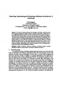
We observed two different perspectives within the relation storage approach: objectcentered [4, 9, 11, 12] and relation-centered [19, 22]. In.object-centered perspective, relation Schemas are generated from given object Schemas, i.e., types and their hierarchy. Relations are the destination for storing objects, and objects are decomposed into relations using the concept of normalization. On the other hand, in relation-centered perspective, object schemas are defined from given relation schemas. Relations are the source for generating objects, and objects are composed from relations. The composition of objects is useful for building object-oriented applications on top of existing relational databases2. The two perspectives may look like the two sides of the same coin, but they differ in terms of design approach. Figure 2.1 shows the two perspectives. In Figure 2.1a, the Project-manager type is mapped to the Project-manager relation. There exists a separate relation for each corresponding object type. In Figure 2.1b, there does not exist a separate Project-manager relation in the given even a file system [21]. 2 We cannot throw away the relational data model in a decade. Remember that the IMS hierarchical data model implementation is still prevalent while we call the relational model 'conventional'.
CHAPTER 2. BACKGROUND FRAMEWORK
Type Employee fis-a Type Project-manager ■Ij-generates Relation Employee(ssn, ...) Relation Project-manager(ssn, ...) (a) Object-centered perspective Type Employee | is-a Type Project-manager ftdefined-from Relation Employee(ssn, ...) Relation Project(..., manager-ssn, ...) (b) Relation-centered perspective Figure 2.1: Two perspectives of relation storage approach database. Rather, the Project-manager type is denned as an abstraction through views, such as defining a join between the Employee relation and Project relation along the manager-ssn foreign key. The join retrieves only the employees that are managing one or more projects. Let us consider the Project-manager as a derived relation of the Employee and Project relations. Note the derived relation is analogous to the intensional database (IDB) relation [32, 34] used in the integration of the logic-based model and relational model [34, 35, 36]. For example, the IDB relation of the Project-manager is written as follows using the notion of Datalog [32]. Project-manager(ssn, • • •)
: -
Employee(ssn, ■ • •) & Project(- • •,manager-ssn, • • •) & ssn = manager-ssn.
We use the relation-centered perspective throughout this thesis but the result is applicable to the object-centered perspective as well, particularly during execution (operationally).
2.4. INSTANTIATING OBJECTS FROM RELATIONS THROUGH VIEWS
2.4
7
Instantiating Objects from Relations through Views
Views provide a user-defined subset of a large database. Thus, as mentioned in Section 2.3, views are used as a tool for providing sharing and abstraction in interfacing between an object-oriented model and the relational model. We also want to use the views for instantiating objects from relations. To achieve this, views should provide mapping between heterogeneous structures of the two models. The mapping is done by linking object attributes to corresponding relation attributes. Objects have a more complex structure than relations. For instance, objects support aggregation hierarchies [88, 72] through an is-part-of relationship3. Hence objects have a nested structure, which is different from nested tuples because the type of an attribute can be a reference to another object. Therefore, given relation attributes, it is difficult to map the relation attributes to object attributes without explicitly specified mapping information. We thus need to extend the views by adding additional component for the mapping, that is, an attribute mapping function. Figure 2.2 shows an example of instantiating objects through such an extended view.
The object type defines the structure of objects to be retrieved from the
database. The query part of the view, what we call a view-query, specifies how to materialize the objects from the relational database. The join between the Employee relation and the Child relation has the semantics of nesting such as "For each Employee tuple, retrieve the matching tuple in the Child relation." The outer relation is called a source relation and the inner relation is called a destination relation in our work. The attribute mapping part of the view shows the aggregation hierarchy of object attributes and their mapping to relation attributes. The mapping is one-to-one as long as there is no derived attribute among the object attributes. We use the key attribute of one of the relations as the source of the object identifier (oid). In Figure 2.2, the key ssn of the Employee relation is retrieved to become the oid of the Employee 3
Objects also support a generalization hierarchy through is-a relationship, inheriting part of the attributes from parent objects. We regarded the inherited attributes as well as the local attributes uniformly as belonging to the objects.
CHAPTER 2. BACKGROUND FRAMEWORK
Database schema: /* Underlined attributes are keys. */ Employeefssn, e_name, sex, degree, salary, dept#) Engineerfssn, specialty, experience) Department(dept #, d_name, manager_ssn, address) Childfssn. c_name. sex, birth-date) Object Type Employee /* [ ] denotes a tuple. */ [name: string, dept: Department, children: [name: string, birthDate: string]] View: • Query expressed in relational algebra: n
{ssn,ejname,dept#,cJiame,birth.date} Employee JC^ Child
• Mapping between object attributes and relation attributes: : is-part-of : maps-to
e
birthDate
ssn e_name dept# c_name birth_date Figure 2.2: An example of instantiating an object type through views
2.5.
OBJECT INSTANTIATION TIME
9
object. Object id's are not explicitly denned in the type definition but assumed to exist implicitly. The dept attribute of an Employee object has type Department. We call an attribute whose type is another object type a reference attribute. In objectoriented paradigm, a reference is implemented with the oid of the referenced object. In our framework, the value of a reference attribute is retrieved from the key of a database relation which is mapped to the oid of the referenced object. Thus, in Figure 2.2, the dept attribute of an Employee object is retrieved from the dept# of the Department relation, if we assume that there exists a type Department whose object id is retrieved from the dept# of the Department relation. The children attribute defines a subobject of the Employee object, and each subobject has its own attributes - name and birthDate. Here a 'subobject' is denned as an object which does not have its own type definition but has its structure contained in another object which again may be a subobject of another object. Like the Employee object, a children subobject is assumed to have its object id, but the object id is not actually retrieved from a database relation. The id's of the children subobjects are needed for a different purpose, which will be discussed in Section 3.4.3.
2.5
Object Instantiation Time
The integration of objects and databases can be distinguished according to another dimension - the binding time [51, 52] of an object type. Given an object type, we define its binding time as the time when its instances are retrieved from databases into an application space. A binding time can be distinguished into early binding and late binding. Early binding is a compiled approach. That is, all instances of an object type are retrieved all at once prior to the usage by an application program. In this sense, the early binding is similar to caching [59, 60] or prefetching [61]. Once all instances of an object type are retrieved, an application does not incur the cost of retrieving the instances of the same object type unless the retrieved instances are invalidated by the change of the data stored in databases. Early binding becomes a feasible idea if an application works in a canned transaction in which it is possible to preanalyze the
CHAPTER 2. BACKGROUND FRAMEWORK
10
Object storage Early binding Late binding
Base relation storage Object-centered Relation-centered View-objects
Table 2.1: View-object framework
set of objects that will be used by an application. On the other hand, there may be a situation in which the loading time for instantiating all instances of an object type is significant but this loading time does not pay off because the application does not use all the retrieved instances. In case only a small subset of the retrieved objects are used, late binding is more appropriate. Late binding is an interpreted approach. That is, instances of an object type are retrieved one at a time on demand during the execution of the application program. Late binding makes it possible for an application to retrieve only the objects that are actually needed during execution and hence takes less main memory space than early binding. However, if all the instances turn out to be used during the execution of an application, late binding strategy becomes worse than early binding by incurring as many object requests to databases as the number of used objects. Note that the early binding incurs the object request only once for a given object type as long as the retrieved instances remain valid. From a system design point of view, we can think of a range of choice between the early binding and the late binding, i.e., between the compiled approach and the interpreted approach. This is analogous to the interpreted-compiled range (IC range) in interfacing the Prolog with relational databases [53]. The criteria of choosing between the I-C range are the execution time and memory space. That is, ideally we want to retrieve the minimum number of objects that are needed by an application at the minimum number of object requests.
2.6
View-object Framework
2.6.
VIEW-OBJECT FRAMEWORK
2.6.1
11
View-objects
In [14], Wiederhold proposed database views as a tool for "connecting between object concepts in programming languages and view concepts in database systems". A view is denned by an external schema at the external level of the ANSI/SPARC architecture [27, 28]. Different groups of users can have different views on the same database. A view has been used as a mechanism for mapping between the- different external Schemas of different user views and the conceptual schema of the entire database in two ways. The goal of the view mechanism is twofold: windowing and security. Users access the same database through different 'windows' defined by different views. Query formulation is simplified by enabling a user to write a query as if a view were just another base relation. At the same time, users are restricted to access only a subset of a database, defined by a view4. The goal of windowing emphasizes using views as a tool for materializing a subset of data from relations, while the goal of security puts more emphasis on using views as a tool for managing a database system. Wiederhold's proposal of view-objects put more emphasis on the goal of windowing, that is, using views as a tool for materializing view-objects from relations. A principal way of storing relations is to normalize them into nonredundant, unambiguously updatable form - Boyce-Codd-normal Form, for example. A materialized view is only in the first normal form and is closer to an 'object' in the sense that related attributes are brought together. For example, the view of the Employee object type in Figure 2.2 brings together, when materialized, the information about an employee and the information about the employee's children. Note that the attributes of an entity denoting a real world object are decomposed into the attributes of normalized relations in a database design process. We can say that a view is used to Ireassemble' the decomposed attributes into the attributes of the entity. Objects that we are dealing with in this thesis are view-objects because the objects are instantiated by materializing a view. In our work, a view-object is a complex object which is implemented by a nested relation and supports references among objects. Table 2.1 illustrates where a view-object belongs to among the two-dimensional 4
It is typical that a database administrator has the privilege of maintaining the security of a database system through this view mechanism by assigning views to each group of users.
12
CHAPTER 2. BACKGROUND FRAMEWORK
categories of the framework that were discussed in Section 2.2 through Section 2.5. The view-object framework belongs to the relation-centered perspective of the relation storage approach. Early binding is assumed, that is, the results of a view-query are retrieved all at once into an application workspace and restructured into objects. The client-server architecture is appropriate for supporting the view-object framework [14]. In this architecture, a subset of the database content residing on a server is retrieved to a client workstation and used to provide objects (after necessary restructuring) during the execution of an application.
2.6.2
Related Work on View-objects
In [14], a view-object generator was proposed as an important component of the system implementing the view-object concept. Based on this proposal, Barsalou et al. [15, 16, 17] implemented a view-object generator in their Penguin project [22, 23, 24]. Besides, Cohen [18] implemented a different kind of view-object generator in his OBI project.
2.6.2.1
Penguin
Penguin is an expert database system being built at the Stanford University for applications in the areas of biomedical engineering, civil engineering, and electrical engineering. In the Penguin project, Barsalou et al. implemented a view-object generator using a structural data model [13]. The structural data model is essentially a relational data model and is augmented with connections. The connections represent interrelational constraints such as referential integrity constraints and cardinality constraints. Barsalou et al. used an object template as a tool for formulating a viewquery. An object template is a data structure with different attributes (or slots). Users formulate a view by designating a pivot relation [16, 17] and selecting connections to follow among the connections to neighboring relations. For manipulating the overlapping views of multiple objects, the object templates are configured into a hierarchy. When an object needs to be instantiated, users select the corresponding object template and specify selection conditions on a set of relations defined in the object
2.6.
VIEW-OBJECT FRAMEWORK
13
template. The system then formulates a SQL query and delivers it to the database. The query result is restructured into view-objects using a NEST [70] procedure. At the time of this writing, a second prototyping of the Penguin project is still ongoing work at the Stanford University. 2.6.2.2
OBI
OBI is a 'Prolog-based view-object-oriented database' designed and implemented at the David Sarnoff Research Center5.
The goal of the OBI project was to design
and implement a Prolog-based hybrid system of relational databases and objectoriented databases. In OBI, Cohen designed a view-object manager and a direct object manager as a dual system. The purpose of the dual approach was to make it possible to move persistent data from relation storage to object storage back and forth.
OBI uses its own data definition and query language for the view-object
manager. The query language is similar to SQL and can express a predicate of domain relational calculus within a query. In its implementation using Prolog, OBI queries are translated into a Prolog goal and is executed by a standard Prolog execution mechanism. Unlike the Penguin view-object generator, no separate NEST procedure is necessary. The view-object manager materializes a nested relation directly out of relational databases.
5
A subsidiary of SRI International
Chapter 3 Outer Joins and Filters in a View-Query 3.1
Introduction
In this chapter, we develop a mechanism for deciding on inner joins or outer joins, and prescribing non-null filters for a view-query. We first formulate our problem in a concrete manner in Section 3.2. Then, we develop a rigorous system model to facilitate the mapping between objects and relations in Section 3.3. The mechanism is developed in Section 3.4. A summary of this chapter follows in Section 3.5.
3.2
Problem Formulation
In this section we first introduce two operators: left outer join and non-null filters. Then, we formulate a problem by exaplaining the motivation, objective, and our approach to the problem.
3.2.1
The Two Operators
In Chapter 1, we mentioned the need for two operators for instantiating objects from relational databases through views: a left outer join and a non-null filter. A left outer 14
3.2. PROBLEM FORMULATION
15
join is different from an inner join in that it retrieves null tuples when there is no matching tuple in the destination relation for a given source relation. A non-null filter is a selection condition for eliminating any nulls of an attribute from a base relation1. Formal definitions of the left outer join and the non-null filter are as follows. Definition 3.2.1 (Left Outer Join) Given two relations R± and R2, a left outer join from Ri to R2, denoted by Ri IX R2, is defined as follows. Ä1[XÄ2 = (Ä1CXÄ2)U((Ä1-nÄ1(Ä1XÄ2)) x A)
(3.1)
where X denotes an inner join, 7TRJ (.RI XIR2) denotes the projection of Ri X R2 on the attributes of R\, and A denotes a null tuple consisting of nulls for all attributes of R2. In other words, R\ [X R2 produces the following set of tuples. ABB
{< *i,*2 > l^i €'Äi Ata G RiM-i.AHi.B} U {< fx,A >\ti € ÄiA ßt2{t2 € Ä2 A h.ABh.B)}
(3.2)
where 8 denotes a comparison operator, i.e., 6 € {, =, 7^}. For the rest of this chapter, we use a small size join symbol (N) to denote a join which can be (has not yet been determined to be) either an inner join (XI) or a left outer join ([X ). Definition 3.2.2 (Non-null filter) A non-null filter is a conjunction of predicates applicable to a base relation R, defined as follows. R.AX ^ null A R.A2 ^ null A • • • A R.A{ ^ null
(3.3)
where Ai, A2, • • ■, A{ are the attributes of R that are not allowed to have nulls.
3.2.2
Motivation
3.2.2.1
Why do we need left outer joins and non-null filters?
Objects are identified by their identifiers (oid's) only. In other words, an object exists even if all its attributes are nulls as long as it has an object id. Let us consider 1
A base relation is the relation defined by the relation schema of a database, neither a view nor an intermediate relation.
16
CHAPTER 3.
OUTER JOINS AND FILTERS IN A VIEW-QUERY
the objects of typ Employee shown in Figure 2.2. An Employee object exists only if it has its oid retrieved from the ssn of the Employee relation. Assuming that the Employee object allows null for its children attribute, what will happen if the join between Employee relation and Child relation is evaluated by an inner join? Any employee tuple that has no matching tuple in the Child relation will be discarded. In other words, any employee without children will not be retrieved. Therefore, we must evaluate the join by an outer join to prevent the loss of employees that do not have children. Furthermore, what we need is not a bilateral outer join but a unilateral outer join, because we are not interested in retrieving a Child tuple that has no matching tuple in the Employee relation, that is, a child without parent. Therefore, a left outer join is adequate assuming that the source, here the Employee, relation is the left hand side operand of the join. We assume the source relation is always on the left hand side of a join and thus use only left outer joins for the rest of this chapter. Now let us assume the Employee objects prohibit nulls for the dept attribute since a department affiliation is required of every employee. As mentioned in Section 2.4, the dept attribute is retrieved from the dept# of the Employee relation. The join between the Employee relation and Child relation is immaterial to the retrieval of dept# attribute. Rather, nulls of the dept# attribute stored in the tuples of the relation Employee should not be retrieved. Therefore, we must filter the Employee relation with a selection condition 'dept# ^ null'. We call this selection condition a non-null filter. We see from the above examples that we frequently need left outer joins to prevent the loss of wanted objects, and non-null filters to prevent the retrieval of unwanted nulls.
3.2.2.2
Why do we want the system to do it?
Null-related semantics of object types are hard to understand and hence likely to induce errors. For example, the Employee type definition shown in Figure 2.2 does not distinguish between the semantics of 'employees and their zero or more children' and the semantics of 'employees with at least one child'. A left outer join is needed for the former while an inner join is needed for the latter. The distinction is entirely
3.2. PROBLEM FORMULATION
the programmer's responsibility.
17
Even if the semantics is clear, it is an effort for
the programmer to determine the left outer joins and non-null filters given an object type and the corresponding view, especially if the view defines many joins. Therefore mechanization of the process is useful.
3.2.2.3
Why do we want to reduce the number of left outer joins and non-null filters?
The view-query is processed more efficiently if we can eliminate a non-null filter 'R.A^ null' without affecting the query result, and thus avoid evaluating unnecessary selection conditions. Sometimes it is known at the semantic level that the column A of a relation R contains no null. An example is when A is the key of R and the entity integrity [40] is preserved. The query also becomes more efficient if we reduce the number of left outer joins and still retrieve the same result. Sometimes left outer joins produce the same tuples as inner joins. For example in Figure 2.2, if every employee has one or more children, then the same tuples are produced by either join method. We know this fact at the semantic level, provided that the system enforces the referential integrity [40] from Employee. ssn to Child, ssn. As another example, let us consider the following directed join graph. Ri —► R2 —> R3 —► Ri
where the join from R2 to A3 is a left outer join and the others are inner joins. If it is known that there always exists a matching tuple of R3 for every tuple of R2, then the result of Äi XR2IX R3XRA is the same as Äi XR2XR3XRA. Now, if we evaluate the join as an inner join, then the optimizer considers the three joins and will choose the most efficient order of joins. Let us assume the join order becomes #4 _> R3 _► R2 _► Rx in the optimal plan. On the other hand, if we evaluate the join as a left outer join, the query optimizer can not consider reversing the order of R2 [X R3 and thus can not obtain the same optimal plan. In general, converting a left outer join to an inner join allows the query optimizer to deal with a larger number of joins. This increases the number of alternative plans but will certainly
18
CHAPTER 3. 0 UTER JOINS AND FILTERS IN A VIEW- Q VERY
never generate less optimal plan than when left outer joins are evaluated as such and, therefore, cannot be reordered.
3.2.3
Problem Statements
Our objective is thus to develop a mechanism for the system to decide whether the joins of a query should be evaluated by inner joins or left outer joins when objects are instantiated from relational databases through views. In addition, the system decides which relations should be filtered through non-null filters. For efficiency reason, the number of left outer joins and non-null filters should be reduced whenever possible.
3.2.4
Our Approach
The heterogeneity of the object-oriented model and the relational model causes several difficulties in mapping between the two models [41]. Hence we cannot expect a simple solution to our problems without a well-defined system model. The system model should satisfy the following criteria. • It provides the context in which we can develop a simple solution to the problem. • It is based on a standard model and can be easily implemented in many existing systems. Given the system model, we develop a mechanism for solving the problem. We use only one parameter that users should provide to the system. It is a non-null option on the object attribute as will be explained in Section 3.3.1. Users do not even have to know what a left outer joins is. To prevent losing nonmatching tuples when nulls are allowed (by default), all joins of a query are initialized to left outer joins. The semantics of the non-null options are interpreted as non-null constraints1 on object attributes, and mapped to corresponding non-null constraints on the query result. Then we replace some left outer joins by inner joins and add non-null filters to some 2
These constraints require the existence of an object attribute given the oid of an object. We would call this constraint as an existence constraint if this term were not already used in [32] to mean the same concept as the referential integrity.
3.3. SYSTEM MODEL
19
relations accordingly. Finally, the number of left outer joins and non-null niters are reduced using the integrity constraints of the data model. The non-null options, and accordingly the non-null constraints, are used as the correctness criterion of the mechanism. Sometimes there appears to be a conflict in determing between a left outer join and an inner join. For example, let us consider two different attributes A and B that are projected from the same relation R. If A has a non-null constraint mapped from a non-null option on an object attribute but B does not have such a non-null constraint, then the join to the relation R must be an inner join for the non-null constraint on A to be satisfied while it does not have to be an inner join for B. In this case, we require the mechanism to make sure that no null value of A is retrieved, even if it also prevents null value of B from being retrieved, and hence determine the join to the relation R to be an inner join. In other words, the mechanism enforces the semantics of non-null options more strongly than the semantics of the default option, which allows nulls. We call this correctness criterion of the mechanism as a non-null correctness criterion.
3.3
System Model
The system model has three elements: an object type model, a view model, and a data model. The object type model defines the structure of objects. No object type model has gained universal acceptance [42, 43]. Therefore we define a model which is common to many existing object-oriented models [1, 6, 8, 4, 5]. Note that we do not deal with methods, but focus only on object structures. The data model uses the relational model proposed by Codd [26]. The view model contains a relational query3 and defines a mapping between objects and relations. We restrict the query to an acyclic select-project-join query with conjunctive join predicates.
3
We do not assume the usage of any specific query language for our work.
20
CHAPTER 3.
Relation Employee
OUTER JOINS AND FILTERS IN A VIEW-QUERY
(ssn) (id) Object Employee
(a) A pivot relation as a base relation Relation Employee
I
ssnMmanager-ssn
1:1
(ssn) (id) Object Project-manager
I.
Relation Project (b) A pivot relation as a derived relation Figure 3.1: The concept of a pivot relation
3.3.1
Object Type Model
Many existing object-oriented models support aggregation through nested structures and references. For example, the Employee object of Figure 2.2 is an aggregation of name, dept, and children where dept is a reference to a Department object, and children is an aggregation of name and birthDate. The children attribute defines an embedded substructure of the Employee object. Thus our object type has a similar structure as the complex object [44, 45, 46]. We use value-oriented object id's [49, 50] and retrieve them from the keys of relations4. Those relations providing object id's are called pivot relations [16, 17]. As discussed in Section 2.3, an object is mapped semantically to a derived relation rather than a base relation if no base relation provides the same semantics as the object type.
Figure 3.1 illustrates these concepts.
In Figure 3.1a, the Employee
relation is the pivot relation for the Employee object and provides its key ssn as the object id. Figure 3.1b shows the derived relation Project-manager of Figure 2.1, which becomes the pivot relation for the Project-manager object. It is defined by Employee ssn=manager-«sn X Project, and the key ssn of Employee in the Jioin result is J * retrieved as the object id. We do not consider derived attributes for our object type. Derived attributes have 4
Tuple identifiers are usable as well. Otherwise we assume the system maintains a mapping between system-generated object id's and the keys of the corresponding relations.
3.3. SYSTEM MODEL
21
no direct mapping to relation attributes and, therefore, are computed separately from relation attributes. An object type is defined formally as a tuple of attributes, [Ax, A2, • • •, X\, X2, • • •] where each A{ is a simple attribute, and each A',- is a complex attribute. Each attribute is either local to the object or inherited from its parent, and we consider both the local and inherited attributes as 'defined' in an object type. An attribute is described in Backus-Naur Form as follows. attribute ::= simple attribute | complex attribute simple attribute ::= internal attribute | external attribute complex attribute ::= [attribute, attribute, ••• ] A simple attribute has an atomic value or a set of atomic values. It is either internal or external to the object. An internal attribute has a primitive data type such as string, integer, etc., while an external (or reference) attribute has another object type as its data type. The value of an external attribute is the oid of the referenced object. A complex attribute defines a subobject or a set of subobjects by embedding its type definition within the object type. In the same way as an object id is mapped from the key of a pivot relation, a subobject also has an associated oid which is mapped from the key of a base relation. However, the oid of a subobject is not retrieved while the oid of its (super)object is retrieved from the key of a pivot relation5. We need a way of telling the system whether the value of an object attribute is allowed to be null or not. This is done by attaching a non-null option to an object attribute. This option deliberately declares that a null value is not allowed for the attribute. It is equivalent to specifying the constraint of 'minimum cardinality > 0' on the attribute6. Attributes without non-null options are allowed to have null values by default. An example is shown in Figure 3.2. The Project attribute defines its own attributes and becomes a subobject of the Programmer object. It has its object id 5
A subobject of an object is not a stand-alone object because it has no object id. Many commercial tools for building object-oriented system applications, KEE[47, 48] for example, support this option. 6
22
CHAPTER 3.
OUTER JOINS AND FILTERS IN A VIEW-QUERY
Type Programmer [ name: string non-null, dept: Department non-null, salary: integer, manager: Employee, task: string, Project: [ title: string non-null, sponsor: string, leader: string, depart: Department non-null ] ] Figure 3.2: An example object type
Programmer
oid name dept salary manager task Project
oid title sponsor leader
dept
Figure 3.3: The O-tree of the Programmer object type mapped from the key of a pivot relation in the same way the Programmer object does. However, only the id's of the Programmer objects are actually retrieved. This Programmer object example will be used throughout the rest of this chapter. Given an object type, we can build a tree consisting of its object attributes. We call such a tree an O-tree and define it as follows. Definition 3.3.1 (O-tree) The O-tree of an object 0 is a tree which has the following properties. • Its root is labeled by l0\ • A leaf is labeled by a simple attribute of the object O. • An intermediate node (non-leaf) is labeled by a complex attribute of the object O. An example of an O-tree is shown in Figure 3.3 for the Programmer type.
3.3. SYSTEM MODEL
23
Here we introduce two functions directly derivable from an object type: an object set (Oset) and an object chain (Ochain). These two functions are used to facilitate mapping between objects and relations. Definition 3.3.2 (Oset) Given an object 0, Oset(0) is denned as a function returning the set of the root of the O-tree and all of its non-leaf descendents. For example, Oset(Programmer) returns {Programmer, Project}. Note that each element of an Oset has its object id mapped to the key of a pivot relation. Definition 3.3.3 (Ochain) Given an object O and a simple attribute s0 of the object 0, 0chain(O,s0) is defined as a function returning the chain of nodes from the root (0) of the O-tree to a descendent node labeled s0, i.e., 0.0\. • • • .0n.s0. For example, Ochain(Programmer, title) returns Programmer.Project .title and Ochain(Programmer, Project) returns Programmer.Project.
3.3.2
Data Model
Integrity constraints [38, 39, 40] are a part of the data model7. Two kinds of integrity constraints are used in our work: referential integrity constraints and entity integrity coststraints. As mentioned in Section 3.2.2.3, these integrity constraints are useful to reduce the number of left outer joins and non-null filters. The referential integrity constraint is defined as follows. Definition 3.3.4 (Referential integrity constraint) A referential integrity constraint from R.A to S.B requires that if R.A is not null then there exists a matching value of S.B. That is: Va € R.A(a = null V 36 € S.B{a = b)) 7
(3.4)
In the Penguin project, which was introduced in Section 2.6.2.1, the connections of a structural data model provide the semantics of necessary integrity constraints, and therefore, integrity constraints need not be specified separately by a database designer.
24
CHAPTER 3.
0 UTER JOINS AND FILTERS IN A VIEW-Q UERY
Let us denote the referential integrity constraint by an arrow as in R.A i—» S.B. Our definition of the entity integrity constraint is more extensive than the definition used in [40]. Definition 3.3.5 (Entity Integrity constraint) An entity integrity constraint requires one or more of the following conditions to be satisfied. • Primary key constraint: R.A^ null if A is the primary key of R*. • Range constraint: If R.A is not null then ai&i R.A 82a2 where a-i,a2 are non-null constants, and 61,62 are ' Emp.name Division.super-division i—* Division.name Proj-Assign.proj >-» Project.proj# Project.dept »—> Dept .name Dept .name i—*• Division.name Project .leader »-» Emp.ssn Emp.dept H-+ Dept .name Project.sponsor ^ Sponsor.name Engineer.ssn •—> Emp.ssn Project-title.proj# *-* Project.proj# (b) Referential integrity constraints The keys of all relations shown in the database schema are disallowed from having nulls. In addition, Emp.dept and Emp.name are prohibited from having nulls. (c) Entity integrity constraints Figure 3.4: A sample database
26
CHAPTER 3.
OUTER JOINS AND FILTERS IN A VIEW-QUERY
Vif!W Mapping part
Pivotdescription ' I
Query part
Attribute mapping function An
Pivot mapping function
1:1
PS
ww
*- Oset
{Ophain}= So-
1:1
Sr
V
: consists of generates : defines
Object
PS: the set of pivots Oset: object set Ochain: object chain So: the set of Ochains of object attributes appearing in the object type Sr: the set of relation attributes appearing in the query
Figure 3.5: Mapping between objects and relations
Programmerl {name,salary,dept} impl^
,,
*\JDeptlJ)
{manager} ""VDivisionL {name}
(deptj ^ iln-Ai on the join result, the materialized join result satisfies this non-null constraint if and only if all the joins are inner joins and Rn is filtered by An ^ null. Proof: // part: If all joins on the join path are inner joins, any nonmatching tuples are discarded. Then, the attribute An in the join result can have nulls only if An is not a join attribute and some tuples of Rn have null An. (If it is a join attribute, any tuple of Rn with null An is discarded by an inner join.) However, tuples with null An are removed from R^ by the given non-null filter. Therefore the constraint is satisfied. Only if part: We prove this part by contradiction. Let us first assume Ri IX Ri+i is a left outer join for some i although the constraint is satisfied and let Ri+i have non-matching tuples. Then a null Rn.An is retrieved from the null tuples appended to the tuples of Ri which have no matching tuples in Ri+i- This contradicts the assumed constraint. Therefore all the joins must be inner joins. Next, let us assume Rn is not filtered by An / null although the constraint is satisfied and all joins are inner joins. Then null Rn.An is retrieved from the nulls stored in Rn.An if An is not a join attribute. This contradicts the assumed constraint. Q.E.D.
3.4.5
Reducing the Number of Left Outer Joins and Nonnull Filters
We can remove unnecessary non-null filters and further reduce the number of left outer joins by using integrity constraints.
3.4.5.1
Removing Unnecessary Non-null Filters
Considering entity integrity constraints, some non-null filters are removed if they are defined on attributes which cannot have null. A typical case is when the attribute is a key (primary key constraint) or any other non-null attribute designated in the schema definition (value constraint). For example, we can remove Empi.name ^ null and Empi.dept ^ null among the four non-null constraints generated in Section 3.4.4
36
CHAPTER 3.
0UTER JOINS AND FILTERS IN A VIEW-Q UERY
because, as it was shown in Figure 3.4c, those two attributes are key attributes and hence prohibited from having nulls. 3.4.5.2
Further Reducing the Number of Left Outer Joins
We can also replace some left outer equijoins by inner equijoins if we consider referential integrity constraints. Since a referential integrity R.A H-> S.B allows R.A to be null, we define a stronger condition by introducing a variable min as follows. Definition 3.4.1 (min) Given a join Ri M Rj, let min*,- denote the minimum number of matching tuples in Rj for each tuple in Ri. Note min^- is not necessarily the same as minji. Besides, some left outer non-equijoins can be replaced by inner non-equijoins if we consider entity intergrity constraints such as range constraints. Using only the semantics of min without considering the instances of relations11, we define the following rules for deciding whether min is greater than zero or not. MIN(Ä..A) denotes the minimum non-null value allowed for R.A, and MAX(R.A) denotes the maximum non-null value allowed for R.A. MIN(Ä.A) and MAX(R.A) are known from the range constraints or value constraints, if there are airy, on R.A. Rule 3.4.2 • Given a single join predicate AOB for the join between two relations Ri and Rj, minjj > 0 if Ri.A is a non-null attribute and one or more of the following conditions are satisfied. # = '=' and Ri.A H-+ RJ.B and the filter /,- on Rj is empty, or 6 = '>' and lSm{Ri.A) > MAX(Rj.B), or 6 = '>' and MIN(J2i.4) > MAX{Rj.B), or 6 = ' 0. 3. For each join path found in Step 1, replace all joins on the path with inner joins. 12
minjj = 0 does not mean that ntiiWj is always equal to zero. Rather, it means that it is not known at the semantic level whether mixnj is greater than zero.
38
CHAPTER 3. O UTER JOINS AND FILTERS IN A VIEW-Q VERY
As an example, in the query of Programmer object, we find a join path from Engineer! to Division! for which all three joins have min > 0. This is because, as shown in Figure 3.4, (1) there are referential integrities Engineer! • ssn ►-> Empi. ssn, Empj.dept •-* Deptj .name, Depti .name i-» Division!. name, (2) there are integrity constraints prohibiting nulls for Engineer 1.ssn, Empj.dept, and Deptj.name, and (3) none of the relations on the join path has a non-empty filter. We also find a join path from Proj-Assign to Project for which the min > 0. All these joins are replaced by inner joins. Note Project! [X Emp2 and Projecta [X Sponsora cannot be replaced by inner joins because Project .leader and Project.sponsor are not non-null attributes.
3.4.6
Summary of the Mechanism
Given a query with initial left outer joins, the overall mechanism developed in Section 3.4 is as follows. Algorithm 3.4.5 (Summary) Input: object type 0, view (query part and mapping part), relations and integrity constratins. Output: the query part prescribed with inner joins, left outer joins, and non-null filters. 1. /* Preprocessing */ (a) Compile the object type O and generate the object set (Oset) and the set of Ochain(0, s0)'s for all the attributes defined in 0. (b) Generate the query and the mapping part, AMF, PMF, and PS, from the view. (c) Derive the mappings between object id's and the keys of pivot relations using Algorithm 3.3.1, and add the result to the attribute mapping function. (d) Initialize all joins of the query as left outer joins.
3.4. DEVELOPMENT OF THE MECHANISM
39
2. /* Replace all joins within derived relations with inner joins. */ For each derived relation {Rb,E) in the set of pivot relations (PS), replace all joins in E by inner joins. 3. For each attribute s0 of the object 0 that has a non-null option, (a) /* Map the non-null option to a non-null constraint on the query result */ i. fi0,n-So := 0chain(0,50) = 0o-0i. • •• .0„.s0. ii. Rp.A := AMF(ü0,n-id). /* A is always the key of Rp. */ iii. If so is a simple attribute then R..B := AMF(fi0,n^o) else R,.B := AMF(fto,n-so-id). /* If s0 is a complex attribute, B is the key of Rt. */ iv. Output the non-null constraint 'Rp.A =£• R,.B\ (b) /* Generate a non-null filter and prescribe a join. */ i. Replace the filter /, on R„ by /, A {B ^ null). /* Generate a non-null filter. */ ii. /* Prescribe a join. */ A. Find all directed join paths from Rp to R„. B. For each path found in' Step 3(b)iiA, replace all joins on the path by inner joins. 4. /* Using the integrity constraint, remove all non-null filters which can be shown to be redundant, and replace left outer joins if they prove to be equivalent to inner joins. */ (a) Remove lR.A ^ null' such that A is a non-null attribute. (b) Find all join paths between pairs of nodes, such as Ri and Rj, whose miiiij > 0.
(c) For each join path found in Step 4b, replace all joins on the path with inner joins.
40
CHAPTER 3.
OUTER JOINS AND FILTERS IN A VIEW-QUERY
Programmer! (name,salary,dept) ■«v i ^-i-~J} j ^- Jmanager} (ti.Aj6jt2.Bj). However, if U.AjBjU.Bj is false, tx $ Fi if t2 G F2 and t2 £ F2 if U G F1 by the definition of join. It contradicts with the given assumption that tj G F\ and t2 G F2. Q.E.D. It will be good in practice to select the join predicate which takes the minimum computation time, such as an equijoin on integer attributes.
72
CHAPTER 4. EFFICIENTLY INSTANTIATING OBJECTS
K AD'
D G' E
#G
&2 02 vk} °^
a
minimal subtree of JT
rooted by v such that the union of the schema of Vi, v2, ■ ■ ■, vk contains the schema of u. ii. Add u := IIu(i>i Xv2 • • • Xvk) to the AP. iii. Mark i>i, v2, • • • ,vk as 'visited'. 4.3.3.5.3
Index creation
Once redundant joins are removed, indexes are created
on the join attribute of each relation fragment except the pivot relation fragment. For example, given the relation fragments of Figure 4.15, indexes are created on DG'E.D, HG.G, A'lL'.A, and LJ.L. KAD' is the pivot relation fragment. Index creation can start only when the entire tuples of a relation fragment are available because a hashing index requires the number of indexed tuples to be known before an index is created. Since the tuples of relation fragments are transmitted in row-wise order, i.e., different tuples from different relation fragments are intermixed, the index creation on relation fragments can start only after all relation fragments are received. Given the structure of the chained bucket hashing index described in Section 4.3.3.4, the algorithm of creating an index is as follows. Algorithm 4.3.11 (Index creation using hashing) Input: a relation fragment Fi, and a join attribute A{ of F{. Output: a chained bucket hashing index on the attribute A; of Fi. Procedure:
76
CHAPTER 4. EFFICIENTLY INSTANTIATING OBJECTS
1. Allocate a bucket header table. 2. Scan the column A{ of F{ linearly. For each scanned value of Fi.Ai, (a) Compute the hashed address h(Fi.Ai) where h is a hashing function. (b) Insert the value of F{.Ai into the hashing index at the address h(Fi.Ai). I* No duplicate checking is done. */ 4.3.3.5.4
Navigational join
Once indexes are created and an assembly plan is
generated, we perform navigational joins on the relation fragments. The navigational join starts from each tuple of the pivot relation fragment and follows the joins of the join tree to find matching tuples from all relation fragments. For example in Figure 4.15, we perform joins starting from each tuple of KAD' and find matching tuples from DG'E and A'lL' respectively. Then, for each matching tuple of DG'E and ' A'lL' found in previous joins, matching tuples are found from HG and LJ respectively. Note that there always exist one or more matching tuples because non-matching tuples have already been discarded in the materialization phase. The set of matching tuples thus found are assembled into a nested tuple according to the assembly plan generated by Algorithm 4.3.10. For example, starting from the third tuple of KAD', [k3a3d5], the following set of matching tuples are found from each relation fragment as the result of navigation. Example 4.3.2 (Matching tuples [k3a3ds]) • [k3a3d5] from KAD'. • [^501 e4] fr°m
DG E
' -
• [hi9i], [fagi] from HG. • [«13*2*3] from A'lL'. • [faj2],[JaJ4] from LJ. D
4.3. DEVELOPMENT OF OBJECT INSTANTIATION METHODS
77
These tuples are assembled into one nested tuple in the last row of Figure 4.15c. Given the assembly plan shown in Example 4.3.1, {k3a3d5} is projected on the projection set KA, [d5g1e4\ is projected on DE. [/ii^i] and [h5gi] are not projected because their projection set is the same as the schema of the relation fragment HG. [0.3^3] from A'lL' is merged with [Z3j2] and [/3j4] from LJ respectively, and projected on IJ to produce \i2j2] and \i2ji)- Duplicate checking is required when the tuples are assembled into a nested tuple because projections may produce duplicate subtuples. Carrying out navigational joins in this way for all tuples of the pivot relation fragment, we obtain the nested relation shown in Figure 4.15c. The following algorithm describes the procedure of a navigational join more rigorously. Algorithm 4.3.12 (Navigational join) Input: relation fragments-Fi,i - 1,2, • • • ,n(.FY is the pivot relation fragment.); indexes on the join attributes of Fi}i = 2,3, • • • ,n; a join tree (JT), a nesting format tree (NFT), and an assembly plan (AP). Output: a single nested relation (SNR). Procedure: 1. Allocate an empty single nested relation SNR. 2. wp := the root of the empty SNR. 3. up := the root of NFT. 4. For each tp € Fi, /* Fi is the pivot relation fragment */. Assemble(tüp, up, tp). Assemble^, Up, tp) starts navigation from tp and collects the set of tuples {U\ti € Fi,i - 2,3, • • • ,n}, that satisfy the join conditions among Fi, F2, • • ■, Fn. Then, it inserts tp and the collected set of matching tuples into a single nested relation. For each insertion, it first finds, from the assembly plan, the set of relation fragments that are to be merged to produce the tuple to be inserted and their associated assembly plan expression. Secondly, the assembly plan expression is executed on those tuples to
78
CHAPTER 4. EFFICIENTLY INSTANTIATING OBJECTS
be merged. Only projection is performed if no merging is prescribed in the assembly plan expression. Thirdly, the resulting tuples are inserted to corresponding nested subrelations. Every insertion is preceded by a searching for checking if there already exists a duplicate tuple. Algorithm 4.3.13 (AssembleJtF) Input: A node (u\) of the SNR, a node («,-) of the NFT, a join tree (JT), an assembly plan (AP), and a tuple t0 from which we start navigation. Output: SNR with newly inserted tuples. Procedure: 1. wT := the node pointed by W{.Ui. /* wT is the root of the binary search tree of the nested subrelation to be searched. */ 2. Find V = {v1,v2,---,vk} from AP such that m = AP^,^, • • • ,vk) . I* k > 1 if and only if a merging is required. */ 3. /* Let Fi be RFJT"1^) for v{ € V, and let $t be the join predicate between Fi and F5 where RFJT(i^) is the parent of RFJT(Fi) in JT. */ /* Find the tuples from FuF2r--,Fk that match t0- */ For each
N/2d, i.e., d > 1/2, all buckets headers are eventually filled, assuming the hash function distributes a hashing key uniformly over the bucket header table. In this case, the ultimate value of Nb becomes N/(N/2d) = 2d. Otherwise, if d < 1/2, only TV bucket headers out of N/2d headers are filled and the ultimate value of Nb becomes 1. As for the intermediate value of Nb in the middle of insertions, we use half of the ultimate value as an expected value. Thus, Nb = MAX (d, i)
(4.20)
The cost of transmitting the inserted tuple is part of the transmission cost and is not included here. Thus, the cost of inserting a hashed tuple into a chain of hashing buckets is computed as a function of T and d as follows. Ctupinsertid, T)
=
d{Cmp + Nh(Cm + Cmp) + Cma + Ccop3/(T) + 2Cmp) + (1 - d)(Cmp + ~(Ccm + Cmp))
(4.21)
where the value of Nb is computed as follows. Using Equation 4.19 and Equation 4.21, the SFR duplicate elimination cost is computed as follows. Nt
Csfrde = Cma + -j-(Ctuphash(Tt) + Ctupinsert{^t,Tt))
(4.22)
The cost of eliminating duplicate tuples from relation fragments Fj, i = 1,2,•■•, n/, is computed as follows.
X
Nt
Crfde = £(Cma + -f-iCtuphaihiTfi ) + Ctupin,„t{dfi, Tfi)))
(4.23)
Since the query result of the SNR method is also a set of relation fragments, its duplicate elimination cost is the same as that of the RF method except that it incurs the additional cost of writing non-duplicate tuples to an output buffer instead of transmitting, them to a client as in the RF method. The cost of writing non-duplicate tuples from a relation fragment F; to an output buffer is C,coPy(7/i)7Vy.. Thus, the cost of eliminating duplicate tuples from Fi, i = 1,2, • • •, nf, to be used in the SNR method is computed as follows. n
t
C.nTde = CTfde + £ CawiTfi )Nti i=i
(4.24)
4.4. DEVELOPMENT OF A COST MODEL
4.4.2.2
93
Nesting Cost
4.4.2.2.1
Binary Search Tree Searching and Insertion Costs
The searching
(Algorithm 4.3.7) and insertion of one tuple (Algorithm 4.3.9) are used commonly for all three object instantiation methods. Hence, we deal with their cost formulas separately here. We assume all binary search trees implementing nested subrelations are well-balanced. In fact, well-balanced trees are common and degenerate trees are very rare [94]. Even if a binary tree should be balanced sometimes, a tree balancing involves only pointer movements and incurs negligible cost. Let M be the number of tuples that are attempted to be inserted into a binary search tree. Every attempt of insertion requires one searching to check if the same tuple has already been inserted into the binary search tree. Let N denote the number of tuples that are actually inserted into a binary search tree. According to Knuth [94], a single searching requires about 1.386log2 k comparisons (k is the number of nodes currently in the binary search tree) for a well-balanced binary search tree, considering both a successful search and an unsuccessful search. If we assume the insertion of the N tuples out of M tuples occurs at a regular interval, the value of k is incremented at every M/N insertion attempts. Then, the total searching cost for inserting N tuples out of the attempted M tuples is computed as follows. N
M
Cun^arcHiM, N) = £( — 1.386Cfa log2 k) k=l iv
(4.25)
Insertion cost is the sum of the cost of an unsuccessful searching and the cost of inserting a node as a leaf of the binary search tree. An unsuccessful searching of a binary search tree requires log2(k +1) comparisons. Node insertion at the leaf requires the allocation of an empty node (Cmo), copying tuple into the node {Ccopy(T)), and writing a pointer to the node in the parent node (Cmp). Thus, the total cost of inserting N tuples to a binary search tree is computed as follows. C^^N, T) = £(Cb5 log2(* + 1) + Cma + Ccopy{T) + Cmp)
(4.26)
fc=i
There will be Nti tuples inserted into a nested subrelation Si of the final output single nested relation. Let S^i) denote the nested subrelation such that NSRNFT(Spor(i))
94
CHAPTER 4. EFFICIENTLY INSTANTIATING OBJECTS
is the parent of NSRNFT(5;). Then, there exist Nt
... binary search trees implement-
ing the nested subrelation Si, i.e., one binary search tree for each tuple of Spar(i). Let Mti denote the number of tuples that are attempted to be inserted into Si. If we assume tuples are uniformly distributed into every binary search tree of Si, MtJN,
,;)
tuples are attempted for insertion and NSi/NSpaT{.. tuples are actually inserted into each binary search tree of Si. Thus, the total cost of inserting Nti tuples into 5; out of the attempted Mti tuples is computed as follows. Ctisearch(Mti,Nti,Ntpar(i)) = iVVr(i)CWn,eflrch(7r^-1 Tz-*-) •N. ..'N. ,., Nt.
CMiinsert(Nsi,Tti,Nlpar(i)) = N^^Cbininserti^:
4.4.2.2.2
SFR Nesting Cost
~ ,TSi)
(4.27)
(4.28)
We consider only the costs of projecting tuples,
searching tuples (Algorithm 4.3.7), and inserting tuples (Algorithm 4.3.8), which are the operations on data tuples and whose costs are dominant. According to Algorithm 4.3.5, Nt tuples are assembled to a single nested relation. Each one of the Nt tuples is decomposed into subtuples belonging to different nested subrelations Si, S2, ■ ■ •, Sn, by projections. For each of the Nt tuples, the projection of the tuple on the schema of Si costs Cproj^T^). The searching of Si for the projected subtuple costs Csitearch(Nt, N,{, Ntpar{i)), and the insertion of the projected subtuple into Si costs Cninsert(Nti,TSi, N,rar{i)). Hence, the total cost of assembling Nt tuples of a single flat relation into a single nested relation is computed as follows. Csfmest = £ (Cpnjtti (T.t) Nt + C,i,eareh(Nt, N«, Nlpar(i)) + C.un.„t(Nti, Tti, Ntfar(i)))
(4.29) 4.4.2.2.3
RF Nesting Cost
We ignore the costs of the join purge step and the
assembly planning step because they are not operations on data tuples. Accordingly, we approximate the RF nesting cost as the sum of the index creation cost and the navigational join cost. Crfnett — Cix„t + CnaVjn
(4.30)
4.4. DEVELOPMENT OF A COST MODEL
95
The number of joins among the relation fragments is always one less than the number of the relation fragments (n/ — 1) after the join purge step. Index creation (Algorithm 4.3.11): For a relation fragment Fi, the cost of bucket header allocation is Cma- The linear scan costs CcoUca^N^). As for the hashing of join column, we assume all join attributes are integers so that no folding is required. For each of the Nj scanned join column values, hashing computation costs Che and insertion to a hashing bucket chain takes the cost of allocating a bucket (Cma), writing a pointer (Cmp) to the tuple containing the hashed attribute, and two pointer writings (2Cmp) to make connections to other buckets. Note we do not need to scan the entire chain of buckets because no duplicate checking is required. Hence, the cost of creating 7i/ — 1 indexes on Fi.A^s for i — 2,3, • • •, nf, where J*\ is the pivot relation fragment, is computed as follows. Cixcrt = ^(Cma + CcoLca^Nft ) + (Chc + Cma + ZCmp)Nfi)
(4.31)
t=2
Navigational join (Algorithm 4.3.12): The allocation of an empty single nested relation costs Cma. As for the assembly cost (Algorithm 4.3.13), we consider only the costs of following operations on data tuples: the cost of finding matching tuples (Algorithm 4.3.14), the cost of executing assembly plans (AP) on the found tuples, and the cost of inserting (Algorithm 4.3.9) the resulting tuples into the single nested relation after checking for duplicate tuples (Algorithm 4.3.7). Matching (Algorithm 4.3.14): The cost of Match(fi, Fj,U.A6tj.B), denoted by Cmatchij, is computed as follows. First, hashing of a join column costs Che- Let Nb denote the expected length of the chain of buckets including the header bucket. Then, in Step 2, it costs Nb(2Cmp + Ce) to follow the chain of buckets - one Cmp for reading a pointer to a tuple tj € Fj, the other Cmp for reading the pointer to next bucket, and Ce for evaluating the join predicate U.AOtj.B. ccij tuples of Fj are collected from Ma.tch(ti,Fj,ti.AOtj.B). The collection of matching tuples incurs only the cost of writing ctij pointers (Cmpa.ij). Thus, the cost of finding matching tuples of Fj for each tuple £{ of Fi is computed as a function of a.ij as follows. Cnatchii K) = 0^ + Nb{2Cmp + C€) + Cmpaij
(4.32)
96
CHAPTER 4. EFFICIENTLY INSTANTIATING OBJECTS
where the value of Nb is obtained as: Nb = MAX(Nf]/Dfi],2)
(4.33)
= MAX (atJ-, 2) by Equation 4.9
(4.34)
• in the same way we obtained the ultimate value of Nb for Equation 4.20. As mentioned in Section 4.3.3.4, we assume the allocate bucket header size is 50% of the cardinality of a hashed relation fragment. The cost of the entire matching process is the sum of the cost of linear scan on the pivot relation fragment {CcoUcan(Nh)) and the cost of finding matching tuples from the other relation fragments. Cmatch = CcoUcaniNfr) -f
^Z
L
ftCmatchi^])
(4.35)
tgLeaf(JT)
where Leaf( JT) denotes the set of the leaves of the join tree JT and Lfi is obtained as follows.
Lu = Nh
JJ
op,
(4.36)
(RFJT( *■,,), RFJT(F,)> e Plt-
where Pu is a path from RFJT(Fj) to RFJT(Fi). Execution of assembly plans (Step 3a of Algorithm 4.3.13):
The tuples of rela-
tion fragments that are found by the matching process are merged according to the prescription of the assembly plan. Let mt- be the number of relation fragments whose tuples are merged to produce tuples to be inserted into a nested subrelation Si, and let T',.,3 = 1,2, • • • ,m.i, denote the size of the attributes projected from each one of the to-be-merged relation fragments. Then, the following equation holds true.
^ = E^.
(4.37)
The case of merging two tuples from two relation fragments requires two projections on the tuples. Extending from this case, the cost ofmerging mi tuples from m; relation fragments into the tuple of a nested subrelation Si is obtained as Yr^i CprOJect(T^.). This formula can be rewritten as a function of Tti and m; using Equation 4.8 and Equation 4.37. CapextCi{Tti,mi) = {im - l)Cjn + .RFT
^
Selectivities
Figure 4.24: Domain HL and domain LH vs. Domain FF (full ranges) 4.5.3.2
Observation using Simulation
We carried out the cost evaluations using random values of data parameters with the same domains as those used in Section 4.5.2, but this time for different domains of a;/s and pfi's. The following two different domains were used for generating random values of a;'s and Pft's. • Domain HL: (Higher values of a^ and lower values of p^.) 5.00 < ai:i < 10.00 for < i,j >e * and 0.00 < pfi < 0.50 for i = 1,2, • • •, 7. • Domain LH: (Lower values of a,j and higher values of pjr) 1.00 < oij < 5.00 for < i, j >e $ and 0.50 < pfi < 1.00 for i = 1, 2, • • •, 7. Figure 4.24 contrasts the Domain HL and Domain LH with the domain of the full range of values of a,j and p}i that were used in Section 4.5.2. Table 4.7 shows the result of cost evaluations. For Domain HL, the RF method showed more favorable result than the result shown in Tables 4.5 in terms of both the average cost and the winning counts than the SFR or SNR method. On the other hand, for domain LH, the RF method showed less favorable result. Thus, we confirmed that the observations made in Section 4.5.3.1 are generally true for other
4.5. COMPARISON OF COSTS
Method SFR RF SNR
Method SFR RF SNR
Average data size 33878 Mbytes 4.1 Mbytes 8.8 Mbytes (a) Domain
111
Partial local processing Transmission #wins #wins Average cost Average cost WAN LAN 30.2 hours 0% 23.5 days 0% 32.0 hours 31.7 sees 100% 93% 14.0 sees 4.1 mins 0% 36.6 sees 7% 29.9 sees 8.8 mins HL (5.00 < a{j < 10.00,0.00 < Pii < 0.50)
Partial local processing Transmission #wins Average cost #wins Average cost Average WAN LAN data size 0.8% 2.0 mins 0% 47.0 Mbytes 2.7 mins 46.9 mins 99.2% 4.0 sees 22% 51.8 sees 0.86 Mbytes 2.9 sees 0% 4.6 sees 78% 0.53 Mbytes 1.8 sees 31.8 sees (b) Domain LH (1.00 < aij < 5.00,0.50 < Pu < 1.00)
(Transmission time is elapsed time and local processing time is CPU time.) Table 4.7: Costs evaluated using random data parameter values with biased o^'s and
112
CHAPTER 4. EFFICIENTLY INSTANTIATING OBJECTS
values of data parametes as well. It is interesting to note that, for Domain LJi, there were some cases in which the SFR method won over the RF method in the partial local processing cost.
4.6 4.6.1
Summary and Future Work Summary
We have developed the mechanisms of three different methods for instantiating objects from a remote relational database server by materializing a view query and restructuring the query result into a nested relation and resolving references among them. The three different methods were the single flat relation (SFR) method, the relation fragment (RF) method, and the single nested relation (SNR) method, named after the data structure transmitted from a server to a client in each method. Rigorous algorithms have been developed for each step of the object instantiation process, mainly focusing on the transmission and the nesting step of the translation, and a partial cost model has been developed. We have excluded the query processing cost and the reference resolution cost to simplify our work, because these two costs are the same in all three methods. We have performed cost comparisons using randomly generated data parameter values; and using sample data parameter values for varying values of a selectivity (a,-,-) and for higher and lower values of extra join attribute ratios
The result of the cost comparison demonstrated that the RF method and the SNR method are more efficient than the common SFR method in terms of .both the transmission cost and the local processing cost. Therefore, the RF and SNR methods are useful not only for remote database systems but also for local database systems. Besides, the RF and SNR methods are useful for disk-storage database systems as well as main memory database systems although the benefit of the RF and SNR methods is relatively less for the disk-storage database systems due to the significant cost of disk accesses. The RF method wins over the SNR method more frequently. Therefore, the RF
4.6. SUMMARY AND FUTURE WORK
113
method is the most preferred method if we have to choose one of the three methods. There remains an optimization issue of choosing between the RF method and the SNR method depending on the query and the speed of a server and a client. (If the server runs slower than the client, it is more favorable to the RF method than the SNR method because the SNR method performs the nesting step on a server. On the other hand, if the server runs faster than the client, it is more favorable to the SNR method. Note that we assumed that the server speed and the client speed are the same for the cost comparison.) We have not considered the possibility of main memory overflow in case the amount of data retrieved as the result of a query exceeds the amount of available main memory space. Concern about main memory overflow does not discourage the use of the RF or SNR method because it is evident that the SFR method will suffer more severely from the shortage of main memory space than the RF or SNR method because the SFR method carries more redundant data.
4.6.2
Future Work
We discuss further work in two directions. First, the improvement of the efficiency of the RF method and the SNR method, and secondly, handling left outer joins in each of the three methods. Remember that we have dealt with only inner joins for a query in this portion of our work. 4.6.2.1
Improving the Efficiency of the RF and SNR Methods
As mentioned in Section 4.3, we placed more effort in making the SFR method efficient than the RF or SNR method because our objective was to demonstrate that the RF method and the SNR method are more efficient than the SFR method. The RF method and SNR method were designed to be rather simple than utmost efficient. We present here some ideas that are worth pursuing to improve the efficiency of the RF method and the SNR method. In the current RF method, a client carries out the index creation and navigational joins on relation fragments and hence a server must send extra join attributes to
114
CHAPTER 4. EFFICIENTLY INSTANTIATING OBJECTS
make those operations possible. As discussed in Section 4.3.5 and demonstrated in Section 4.5.3.1, extra join attributes are the source of redundant data in the RF method. One idea for avoiding the transmission of the extra join attributes is to have a server send the necessary linkage information in the form of physical pointers to the linked tuples of the other relations. In order to map between the heterogeneous address spaces of a server and a client, offset addresses can be used as long as it can be ensured that each relation fragment is allocated in a contiguous memory space. Sending physical pointers will reduce the transmission cost by not sending extra join attributes and the redundant tuples introduced by the extra join attributes. Moreover, all a client has to do is to follow the pointers to build a single nested relation out of the relation fragments. Thus, it reduces the load on a client. However, a server has to pay the price of index creation and navigational join to produce the physical pointers. A direct consequence of this requirement is that the duplicate elimination step cannot be pipelined with the transmission of tuples and more load is placed on a server. Besides, the transmission protocol becomes more complicated because, unlike the case of sending extra join attributes, the number of physical pointers attached to each tuple varies depending on the number of matching tuples. As for the SNR method, the current SNR method has the overhead of dealing with multiply occurring subtuples in nested subrelations.
One idea of eliminating
these multiply occurring subtuples is to achieve more compaction of the transmitted data by using backward pointers embedded in the formatted stream of nested tuples. These backward pointers replace the actual tuples with pointers to the previously sent identical tuples. It will make the transmission protocol and the assembly process (Algorithm 4.3.16) more complicated, but will reduce the transmission cost. The two ideas described so far have their major benefit in reducing the transmission cost. Therefore, these ideas are more useful in the wide area network (WAN) environment where the transmission cost is the dominant cost. Finally, we have used the RF materialization as an intermediate step of the SNR materialization because, as mentioned in Section 4.3.1, a direct materialization disables the join reordering by a query optimizer. It will be worthwhile to compare the cost reduction achievable by using the direct materialization of a single nested
4.6. SUMMARY AND FUTURE WORK
115
relation and the cost reduction achievable by utilizing the join reordering available from a query optimizer. 4.6.2.2
Handling Left Outer Joins
We have simplified our work by not considering left outer joins in a query although left outer joins are required frequently to prevent information loss. Thus, it will make our work more complete if we discuss the handling of left outer joins in each step of the different object instantiation methods, before ending this chapter. Since we designed the SNR method using the same query materialization and nesting processes as the RF method, we discuss only the SFR method and the RF method. The consideration of left outer joins requires the handling of non-matching tuples in the join evaluations of the query materialization step, and the processing of null tuples in subsequent steps. We state briefly the key points of handling left outer joins at each step. In the SFR method, the query processing algorithm described in Algorithm 4.3.1 should be modified so that if a join is a left outer join and there exists no matching tuple in the destination relation, null tuples are inserted in place of the tuples of the destination relation and its child relations in the join tree. For each U € Ri if U satisfies $i then continue else Set U and all t,- € Rj's to null where Rj, j ^ i, are the relations in the subtree of the join tree rooted by Ri\ Continue, where 'continue' means to continue the nested loop join on the rest of the relations that have not yet been processed. On the other hand, in the RF method, the query processing algorithm described in Algorithm 4.3.2 should be modified so that if a join is a left outer join and there exists no matching tuple in the destination relation, the joins in a subtree of the join tree rooted by the destination relation are skipped. Consequently, no null subtuple is inserted to any relation fragment. For each U E Ri
116
CHAPTER 4. EFFICIENTLY INSTANTIATING OBJECTS
if U satisfies $, then continue else Skip all Rj's where Rj,j / i, are the relations in the subtree of the join tree rooted by Ä,-; Continue.
Duplicate elimination process is the same as Algorithm 4.3.3. A single nested relation which is produced by the nesting step does not contain null subtuples at all. Therefore, the SFR nesting step as described in Algorithm 4.3.5 should be modified so that any decomposed subtuple all of whose column values are nulls is discarded. To achieve this modification, we should place 'If U = A (a null tuple) then return.' in front of l
wr := the root pointed by Wi.Ui
which is the first line of Algorithm 4.3.6. The RF nesting needs some modifications as well. First of all, the join purge of Section 4.3.3.5.1 is not applicable to a left outer join. Theorem 4.3.1 does not hold for dangling tuples in the source relation of a left outer join. For example, given a left outer join Fx
IX
pi A p2 • ■ •
A Pi
F2 from a relation fragment Fx to another relation fragment ° e
F2 with conjunctive join predicates p^ A p2 A • • • A pk, it. is possible that some of the dangling tuples in Fx appear to have matching tuples in F2 if only one of pj,p2 ■ ■ ■ ,pk is evaluated, while in fact there exists no matching tuple for a conjunction of all join predicates, px A p2 A • • • A pk. The assembly planning step (Section 4.3.3.5.2) and the index creation (Section 4.3.3.5.3) step need no modification because they have nothing to do with join evaluations. On the other hand, the navigational join step (Section 4.3.3.5.4) performs join evaluations and thus should be modified to distinguish between inner joins and left outer joins. Algorithm 4.3.14 (Match) always returns one or more matching tuples if the evaluated join is an inner join but may return no matching tuple if the evaluated join is a left outer join.
Accordingly,
Algorithm 4.3.13 should be modified so that if Match(*i_!, Fi} $;) returns no matching tuple and the evaluated join is a left outer join then skip the rest of the 'for each' statements and set ti,ti+i, ■ • ■ ,tk to nulls before executing Step 3a through Step 3d.
4.6. SUMMARY AND FUTURE WORK
117
If we had considered the effect of nulls generated by left outer joins in our work, the result of cost comparison would have appeared to be even more favorable to the RF method and the SNR method. The reason is that, in a single flat relation, nulls are duplicated in the same way the other tuples (which are not nulls) are duplicated. Note that there is no duplicate tuple in a relation fragment or a single nested relation.
Chapter 5 Conclusion In this thesis, we addressed two problems - outer join and instantiation efficiency - in the view-object framewprk, i.e., in the framework of instantiating objects from relational databases through views. First, we introduced the view-object framework starting from a general framework of integrating objects and databases. Then, given the framework, we made three major contributions as summarized below.
• We defined a rigorous system model in order to embody the concept of interfacing between objects and relations. The system model consists of three parts: an object type model, a data model, and a view model. An object type defines the nested structure of objects. The non-null option is used to specify object attributes that are prohibited from being nulls. Data model uses the relational model and includes integrity constraints as part of the model. A view consists of a relational select-project-join query and an attribute mapping function for mapping between object attributes and relation attributes. It was beyond our scope to formulate a query or derive an attribute mapping function for a given view, so that we assumed that a query and an attribute mapping function were predefined in each pertinent object type. The system model thus developed provided the basis for developing a simple solution to the outer join problem and a part of the system model was used for the instantiation efficiency problem as well. 118
119
• We developed a mechanism for having the system decide which join should be an inner join and which join should be a left outer join, given a view-query, and generate non-null filters on the relations specified in the view-query. Users are required only to specify non-null constraints on object attributes whose values should not be null. All joins in a view-query are initialized as left outer joins. Those non-null constraints on object attributes are mapped to non-null constraints on relation attributes of the query result. The non-null constraints on relation attributes are then used to prescribe non-null filters on the attribute of base relations and replace left outer joins sitting on the join path from a pivot relation to the non-null constrained relations by inner joins. The remaining left outer joins are further reduced into inner joins if certain integrity constraints are satisfied. Besides, unnecessary non-null niters are eliminated. • We developed two new methods of instantiating objects from remote relational databases, which are far more efficient than the conventional method of retrieving a single flat relation (SFR). One of the two new methods retrieves a query result as a set of relation fragments (RF's). The other method retrieves a query result as a single nested relation (SNR). We called the two new methods as the RF method and the SNR method while we called the conventional method as the SFR method. The algorithms of the three object instantiation methods (SFR, RF, and SNR) were described rigorously. Then, we derived cost formulas based on the algorithms and compared the estimated costs of the three methods. Two techniques were used for cost comparison: sample case test and simulation. The cost comparison result showed that the RF method and the SNR method are far more efficient than the SFR method for both the transmission cost and the local processing cost.
Appendix A Measurement of Cost Parameters The values of cost parameters were measured using programs that are sufficiently realistic to be part of an actual implementation.
As mentioned in Section 4.4.1.1, we
use CPU time for main memory cost and an elapsed time for network communication cost.
A.l
Main Memory Cost parameters
We used Unix clock system call for measuring the CPU time of the elementary main memory operations shown in Table 4.1. The time resolution of the clock is 1/60 seconds while main memory operations take as little as a few microseconds. The poor resolution of clock made it impossible to measure the precise values of main memory cost parameters. Moreover, the execution time varies every time the same code is run, depending on the system load. Thus, we obtained the values shown in Tables 4.1 by repeating the same code one million times and computing an average value. The cost parameter value varies depending on how many subprocedures are called during execution. We can actually define as many subprocedures as we want. According to our experiment on Sun-3, the invocation of a subprocedure which requires four arguments took about 5 to 6 (isecs, which is a large amount of time for a main memory operation. Thus, we excluded the effect of subprocedure invocation from 120
A.l. MAIN MEMORY COST PARAMETERS
121
our measurement by writing a dummy subprocedure requiring the same set of input parameters as a counterpart for each subprocedure and subtracting the time required to invoke dummy subprocedures from the total time. This approach means that our cost parameter values are the minimum values considering only the 'plain' code execution time. One exception is that we did not subtract a subprocedure invocation time if we judged that the code must use a subprocedure, intrinsically independently of who writes the code. Now we comment on some details of how each cost parameter was obtained. • Cb„: We used an implementation of Algorithm 4.3.7 for tuple sizes of 100 to 500 bytes. Tuples were initialized with pseudo-randomly generated base-64 ASCII strings.
The values of Cb„ using those random tuples were measured to be
independent of the tuple size. • Cm: We measured the time for comparing two tuples of size 100 to 500 bytes where each tuple was initialized with pseudo-random base-64 ASCII string, and obtained the same value independently of the tuple size. • Cd, Cd,: We measured the time for copying a tuple of size 100 to 1000 bytes. The measured time was linear with respect to the tuple size. • Ce: The time for evaluating equijoins on attributes of type integer was measured using a code written for more general joins including non-equijoins on noninteger attributes.
We used the type integer because it frequently happens
that joins are performed on key attributes and the key attributes are integers. We used the address of the join attributes, and their sizes and types as input parameters and did not count the time for obtaining those values themselves. • Cff. Folding was done by dividing a tuple into integer segments and adding up the values of the segments. The tuple size used was 100 to 500 bytes. The measured time was proportional to the tuple size. • Che: We measured the time for hashing computation on a psedo-randomly generated integer hashing key using two different hashing methods: the division
122
APPENDIX A. MEASUREMENT OF COST PARAMETERS
method and the multiplicative hashing method [94]. The value shown in Table 4.1 is for the multiplicative hashing method. • Cma: Our experiment showed that Unix memory allocator (malloc) takes about 130 fisec on Sun-3 without regard to the allocated memory size while the other main memory operations takes only a couple of tens of miscroseconds. Therefore, if we used malloc for our work, the memory management cost would become dominant. However, it is a common practice to pre-allocate a working space [9, 96] to facilitate faster memory allocation and garbage collection. Then, memory allocation takes only the cost of moving a stack pointer within the preallocated working space as long as the working space need not be expanded. We assumed the usage of a working space mechanism. • Cmp: The time for reading or writing a pointer value is so small that it hardly affects the cost computation result. Nevertheless we use it for completeness. • Cpi, Cpb: We measured time for projecting a tuple of size 500 bytes on a varying number of 32 byte columns. The measured time was proportional to the total size of projected subtuple. • Cai, CBn: We measured the costs of reading a join column of size 8 bytes while scanning a relation, and computing an integer hashing key from the read column value. The size of a column (8 bytes) are reasonable because it is likely that join attributes are of type (short or long) integer. We assumed tuples are allocated contiguously within main memory. The measured time was linear with respect to the number of scanned tuples.
A.2
Network Communication Cost Parameters
The values of network communication cost parameters (Ci, Cb) depend on the communication media. It is well known that the data rate is 10 Mbps for Ethernet [65] used in the LAN environment. Cheriton and Williamson [69] measured the communication latency (C/) and the per-byte communication cost (Cb) on an idle 10 Mbps Ethernet
A.2. NETWORK COMMUNICATION COST PARAMETERS
123
connecting two SUN-3/75's, and obtained Ci = 2.23 msec and Cb = 1.8/isec. As for the WAN, in [66] it is stated that the data rate is about 56 Kbps for the highest speed leased phone line in normal use while 1.544 Mbps Tl NSFnet [67, 68] lines are used in a few places where the high cost (in terms of financial investment) is acceptable. However, the current status of technological development has come to the point that Tl lines are in practical usage for the NSFnet and the availability of T3 lines (45 Mbps) is promised in near future. We measured the elapsed time for transmitting data from a SUN-3/60 on the Stanford University Ethernet LAN to another SUN-3/60 on the same LAN, and also to a SUN-4 on the University of Illinois via the Tl NSFnet WAN. The client part of the code repeated the transmission of different amounts of data (0, IK, 4K, 8K, 12K, 16K bytes of data plus 10 bytes of header) 60000 times and averaged the measured round trip times. The server part of the code was written to send an acknowledgement so that the client part can measure the round trip time. The measured time is from main memory to main memory. It does not include any disk access cost but does include main memory execution time for iterations, buffer pointer movements, and sending an acknowledgement. Figure A.l shows the average elapsed round trip times measured for vaying data sizes on the LAN and the WAN, respectively. The measured round trip times were almost linear with respect to the amount of transmitted data. We computed the (approximate) values of the two communication cost parameters, C\ and Cb, by equating the measured round trip times to 2 * Ci + Cb x Size for different values of Size = 10, 1034, 4106, 8202, 12298, and 16394 bytes. (We did not use 12298 and 16394 bytes for the WAN.)
124
APPENDIX A. MEASUREMENT OF COST PARAMETERS
Average elapsed round trip time (msec)
jg— Data size (Kbytes) (a) Local area network (on the Stanford Ethernet) Average elapsed round trip time (msec)
jg— Data size (Kbytes) (b) Wide area network (between the Stanford and the Illinois) (The size of transmistted data is 10 bytes (header) larger than the data size.)
Figure A.l: Average round trip time vs. data size on the LAN and WAN
Bibliography [1] F. Bancilhon, et al, "The Design and Implementation of 02, an ObjectOriented Database System," in 'Advances in Object-Oriented Database Systems', Springer-Verlag, September 1988. [2] 0. Deux, et al., "The Story of 02," IEEE Transactions on Knowledge and Data Engineering, vol. 2, no. 1, March 1990, pp. 91-108. [3] R. Agrawal, and N. Gehani, "ODE (Object Database and Environment): The Language and the Data Model," Proceedings of the ACM SIGMOD International Conference on Management of Data, Portland, Oregon, May-June 1989. [4] D. Maier, and J. Stein, "Development of an Object-Oriented DBMS," Proceedings of the OOPSLA International Conference on Object-Oriented Programming Systems, Languages, and Applications, September 1986, pp. 472-482. [5] S. Ford, et al., "Zeitgeist: Database Support for Object-Oriented Programming," Proceedings of the International Workshop on Object-Oriented Database Systems, 1988, pp. 23-42. [6] W. Kim, N. Chou, and J. Garza, "Integrating an Object-Oriented Programming System with a Database System," Proceedings of the OOPSLA International Conference on Object-Oriented Programming Systems, Languages, and Applications, September 1988, pp. 142-152. [7] W. Kim, J. Garza, N. Ballou, and D. Woelk, "Architecture 'of the OIRON NextGeneration Database System," IEEE Transactions on Knowledge and Data Engineering, vol. 2, no. 1, March 1990, pp. 109-124. 125
126
BIBLIOGRAPHY
[8] D. Fishman, et al, "Iris: An Object-Oriented Database Management System," ACM Transactions on Office Information Systems, vol. 5, no. 1, January 1987, pp. 48-69. [9] K. Wilkinson, P. Lyngbaek, and W. Hasan, "The Iris Architecture and Implementation," IEEE Transactions on Knowledge and Data Engineering, vol. 2, no. 1, March 1990, pp. 63-75. [10] M. Stonebraker, and L. Rowe, "The Design of POSTGRES," Proceedings of the ACM SIGMOD International Conference on Management of Data, 1986, pp. 340-354. [11] M. Stonebraker, L. Rowe, and M. Hirohama, "The Implementation of POSTGRES," IEEE Transactions on Knowledge and Data Engineering, vol. 2, no. 1, March 1990, pp. 125-142. [12] T. Learmont, and R. Cattell, "An Object-Oriented Interface to a Relational Database," Proceedings of the International Workshop on Object-Oriented Database Systems, 1987. [13] G. Wiederhold, "Database Design (2nd ed.)," McGraw-Hill Book Company, 1983. [14] G. Wiederhold, "Views, Objects, and Databases," IEEE Computer, December 1986, pp. 37-44. [15] T. Barsalou, W. Sujansky, and G. Wiederhold, "Expert database systems in medicine—The PENGUIN project", Proceedings of the AAAI Spring Symposium on AI in Medicine, Stanford University, CA, March, 1990, pp. 14-18. [16] T. Barsalou, and G. Wiederhold, "Complex objects for relational databases", Computer Aided Design (Special issue on object-oriented techniques for CAD), vol. 22, no. 8, 1990, pp. 458-468.
BIBLIOGRAPHY
127
[17] T. Barsalou, "View objects for relational databases", Ph.D. thesis, Medical Information Sciences Program, Stanford University, 1990. (Also published as a technical report No. STAN-CS-90-1310, Computer Science Department). [18] B. Cohen, "Views and Objects in OBI: A Prolog-based View-Object-Oriented Database," Technical report TR.PRRL-88-TR-005, SRI, March 1988. [19] G. Wiederhold, T. Barsalou, and S. Chaudhuri, "Managing Objects in a Relational Framework," Technical report CS-89-1245, Stanford University, January 1989. [20] A. Paepcke, "PCLOS: A Flexible Implementation of CLOS Persistence," Proceedings of the European Conference on Object-Oriented Programming, Oslo, Norway, August 1988. [21] Personal communication with Andreas Paepcke, Hewlett-Packard Labs., Palo Alto, California, November 1990. [22] K. Law, G. Wiederhold, T. Barsalou, N. Siambela, W. Sujansky, D. Zingmond, and H. Singh, "An Architecture for Managing Design Objects in a Sharable Relational Framework," International Journal of Systems Automation, Research and Applications, International Society for Productivity Enhancement. [23] K. Law, G. Wiederhold, T. Barsalou, N. Siambela, W. Sujansky, and D. Zingmond, "Managing Design Objects in a Sharable Relational Framework," Proceedings of the ASME International Conference on Computers in Engineering, Boston, MA, 1990. [24] K. Law, T. Barsalou, and G. Wiederhold, "Management of Complex Structural Engineering Objects in a Relational Framework," Engineering with Computers, 6:81-92, 1990. [25] W. Rubenstein, M. Kubicar, and R. Cattell, "Benchmarking Simple Database Operation," Proceedings of the ACM SIGMOD International Conference on Management of Data, May 1987.
128
BIBLIOGRAPHY
[26] E. Codd, "A Relational Model of Data for Large Shared Data Banks," Communications of the ACM, vol. 13, no. 6, June 1970. [27] D. Tsichritzis, and A. Klug (eds.), "The ANSI/X3/SPARC DBMS Framework: Report of the Study Group on Data Base Management Systems," Information Systems 3, 1978. [28] D. Jardine (ed.), "The ANSI/SPARC DBMS Model," Proceedings of the Second SHARE Working Conference on Data Base Management Systems, Montreal, Canada, April 26-30, 1976. [29] R. Haskin, and R. Lorie, "On Extending the Functions of a Relational Database System," Proceedings of the ACM SIGMOD International Conference on Management of Data, June 1982, pp. 207-212. [30] R. Lorie, and W. Plouffe, "Complex Objects and Their Use in Design Transactions," Proceedings of the IEEE Annual Meeting-Database Week: Engineering Design Applications, May 1983, pp. 115-121. [31] K. Dittrich, and R. Lorie, "Object-oriented Database Concepts for Engineering Applications," Technical report RJ 4691 (50029), IBM Research Laboratory, San Jose, CA 95193, May 1985. [32] J. Ullman, "Principles of Database and Knowledge-Base Systems," Computer Science Press, 1988. [33] J. Ullman, "Database Theory-Past and Future," Proceedings of the ACM SIGACT-SIGMOD Symposium on Principles of Database Systems, San Diego, March 1987. [34] K. Morris, J. Ullman, and A. Van Gelder, "Design Overview of the NAIL! System," Proceedings of the International Logic Programming Conference, 1986. [35] S. Tsur, and C. Zaniolo, "LDL: A Logic-based Data-Language," Proceedings of the 12th International Conference on Very Large Data Bases, Kyoto, August 1986.
BIBLIOGRAPHY
129
[36] D. Chimenti, A. O'Hare, R. Krishnamurthy, and C. Zaniolo, "An Overview of the LDL System," IEEE Data Engineering, vol. 10, no. 4, December 1987. [37] C. Date, "The Outer Join," Proceedings of the 2nd International Conference on Databases, Cambridge, Britain, September 1983. [38] E. Codd, "Extending the Relational Database Model to Capture More Meaning," ACM Transactions on Database Systems, vol. 4, no. 4, December 1979. [39] C. Date, "Referential Integrity," Proceedings of the 7th International Conference on Very Large Data Bases, Cannes, France, September 1981, pp. 2-12. [40] C. Date, "An Introduction to Database Systems," vol. 1, Fourth edition, Addison-Wesley Publishing Company, Inc., 1986. [41] F. Bancilhon, "Object-Oriented Database Systems," Invited lecture, Proceedings of the 7th ACM SIGART-SIGMOD-SIGACT Symposium on Principles of Database Systems., Austin, Texas, March 1988. [42] D. Maier, "Why Isn't There an Object-Oriented Data Model?," Proceedings of the IFIP 11th World Computer Congress, San Francisco, California, September 1989. [43] J. Joseph, S. Thatte, C. Thompson, and D. Wells, "Report on the ObjectOriented Database Workshop," SIGMOD Record, vol. 18, no. 3, September 1989. [44] W. Wilkes, P. Klahold, and G. Schlageter, "Complex and Composite Objects in CAD/CAM Databases," Proceedings of the 5th IEEE International Conference on Data Engineering, Los Angeles, February 1989. [45] P. Buneman, S. Davidson, and A. Watters, "A Semantics for Complex Objects and Approximate Queries," Proceedings of the ACM Symposium on Principles of Database Systems, 1988.
130
BIBLIOGRAPHY
[46] W. Kim, J. Banerjee, and H. Chou, "Composite Object Support in an ObjectOriented Database System," Proceedings of the OOPSLA International Conference on Object-Oriented Programming Systems, Languages, and Applications, October 1987, pp. 118-125. [47] "IntelliCorp KEE™ Software Development System User's Manual," Document no. 3.0-U-l, Intellicorp, July 1986. [48] R. Kempf, and M. Stelzner, "Teaching Object-Oriented Programming with the KEE System," Proceedings of the OOPSLA International Conference on ObjectOriented Programming Systems, Languages, and Applications, October 1987, pp. 11 - 25. [49] S. Khoshafian, and.G. Copeland, "Object Identity," Proceedings of the OOPSLA International Conference on Object-Oriented Programming Systems, Languages, and Applications, 1986. [50] S. Abiteboul, and P. Kanellakis, "Object Identity as a Query Language Primitive," Proceedings of the ACM SIGMOD International Conference on Management of Data, Portland, Oregon, May-June 1989. [51] G. Wiederhold, "Binding in Information Processing," Technical report no. STAN-CS-81-851, Department of Computer Science, Stanford University, Stanford, CA 94305, May 1981. [52] T. Pratt, "Programming Languages: Design and Implementation (2nd ed.)," Prentice-Hall, Inc., 1984. [53] T. O'Hare, and A. Sheth, "The Interpreted-Compiled Range of AI/DB Systems," Technical Memo (unpublished), Paoli Research Center, Unisys Corp., July 1988. [54] S. Ceri, G. Gottlob, and G. Wiederhold, "Interfacing Relational Databases and Prolog Efficiently", IEEE Transactions on Software Engineering, February 1989.
BIBLIOGRAPHY
131
[55] S. Finkelstein, "Common Expression Analysis in Database Applications," Proceedings of the of ACM SIGMOD International Conference on Management of Data, 1982. [56] M. Jarke, "Common Subexpression Isolation in Multiple Query Optimization," in W. Kim, D. S. Reiner, and D. S. Batory (eds), 'Query Processing in Database Systems,' Springer, 1984, pp. 191-205. [57] P. Larson, and H. Yang, "Computing Queries from Derived Relations," Proceedings of the of the 11th VLDB International Conference on Very Large Databases, August 1985. [58] T. Sellis, "Multiple-Query Optimization," ACM Transactions on Database Systems, vol. 13, no. 1, March 1988, pp. 23-52. [59] A. Sheth, D. Buer, S. Rüssel, and S. Dao, "Cache Management System: Preliminary Design and Evaluation Criteria," Technical Memo TM-8484/000/00, West Coast Res. Center, Unisys Corp., 2400 Colorado Avenue, Santa Monica, CA 90406, October 1988. [60] M. Nelson, "Caching in the SPRITE Network File System," PhD Thesis, University of California at Berkeley, March 1988. [61] H. Wedekind, and G. Zoerntlein, "Prefetching in Real time Database Applications," Proceedings of the of ACM SIGMOD International Conference on Management of Data, 1986. [62] G. Dill, "Peripheral Semiconductor Storage - A Feasible Alternative To Disk and Tape?," Hardcopy, vol. 7, no. 1, January 1987. [63] B. Lee, and G. Wiederhold, "Outer Joins and Filters for Instantiating Objects from Relational Databases through Views," Technical Report no. 30, Center for Integrated Facility Engineering (CIFE), Stanford University, May 1990. [64] P. Dwyer, and J. Larson, "Some Experiences with a Distributed Database Testbed System," IEEE Proceedings, vol. 75, no. 5, May 1987, pp. 633-648.
132
BIBLIOGRAPHY
Also appear in Gupta, A. (ed.), 'Integration of Information Systems: Bridging Heterogeneous Databases,' IEEE Press, 1989. [65] A. Tanenbaum, "Computer Networks," 1st edition, Prentice-Hall, Inc., Englewood Cliffs, New Jersey 07632, 1981. [66] A. Tanenbaum, "Computer Networks," 2nd edition, Prentice-Hall, Inc., Englewood Cliffs, New Jersey 07632, 1981. [67] D. Comer, "Internetworking with TCP/IP: Principles, Protocols and Architecture," Prentice-Hall, Inc. 1988. [68] S. Reddy, "NSFnet Today: A New Implementation of a Vast Research Network" LAN Magazine, June 1989. [69] D. Cheriton and C. Williamson, "Network Measurement of the VMTP RequestResponse Protocol in the V Distributed System," Proceedings of the ACM SIGMETRICS Conference on Measurement and Modeling of Computer Systems, Banff, Alberta, Canada,' May 1987, pp. 216-225. [70] P. Fischer, and S. Thomas, "Operators lor Non-First-Normal-Form Relations," Proceedings of the IEEE COMPSAC International Computer Software and Application Conference, November 1983. [71] M. Roth, H. Korth, and A. Silberschatz, "Theory of Non-First-Normal-Form Relational Databases," Technical report no. TR-84-36, Department of Computer Science, University of Texas at Austin, Austin, Texas 78712, December 1984. < in TODS on "Nested relations'^ [72] S. Abiteboul, and N. Bidoit, "Non-First Normal Form Relations to Represent Hierarchically Organized Data," Proceedings of the ACM SIGACT-SIGMOD Symposium on Principles of Database Systems, April 1984. [73] D. Bitton, "The Effect of Large Main Memory on Database Systems," Panel report, Proceedings of the ACM SIGMOD International Conference on Management of Data, 1986, pp. 337-339.
BIBLIOGRAPHY
133
[74] A. Ammann, M. Hanrahan, and R. Krishnamurthy, "Design of a Memory Resident DBMS," Proceedings of the IEEE COMPCON Conference, San Francisco, February 1985 [75] K. Whang, et al., "OfBce-By-Example, An Integrated Office System and Database Manager," ACM Transactions on Office Information Systems, vol. 5, no. 4, October 1987, pp. 393-427. [76] T. Lehman, and M. Carey, "A Study of Index Structures for Main Memory Database Management Systems," Proceedings of the of the 12th International Conference on Very Large Data Bases, Kyoto, August, 1986, pp. 294-303. [77] T. Lehman, and M. Carey, "Query Processing in Main Memory Database Management Systems," Proceedings of the ACM SIGMOD International Conference on Management of Data, 1986, pp. 239-250. [78] H. Garcia-Molina, R. Lipton, and J. Valdes, "A Massive Memory Machine," Proceedings of the IEEE COMPCON Conference, 1984. [79] D. Bitton and C. Turbyfill, "Performance Evaluation of Main Memory Database Systems," Technical Report 86-731, Department of Computer Science, Cornell University, Ithaca, New York, January 1986. [80] D. Bitton, M. Hanrahan, and C. Turbyfill, "Performance of Complex Queries in Main Memory Database Systems," Proceedings of the IEEE 3rd International Conference on Data Engineering, 1987, pp. 72-81. [81] M. Eich, "MARS: The Design of a Main Memory Database Machine," Proceedings of the 5th International Workshop on Database Machine, Karuizawa, October 1987. [82] A. Swami, "Optimization of Large Join Queries," Ph.D. Thesis, Report no. STAN-CS-89-1262, Department of Computer Science, Stanford University, 1989. [83] E. Horowitz, and S. Sahni, "Fundamentals of Data Structures," Computer Science Press, Inc., 1976.
134
BIBLIOGRAPHY
[84] W. Mauer, and T. Lewis, "Hash Table Methods," ACM Computing Surveys, vol. 7, no. 1, March 1975, pp. 5-20. [85] K. Whang, and R. Krishnamurthy, "Query Optimization in a Memory-Resident Domain Relational Calculus Database System," ACM Transactions on Database Systems, vol. 15, no. 1, March 1990. [86] D. DeWitt, R. Katz, F. Olken, L. Shapiro, M. Stonebraker, and D. Wood, "Implementation Techniques for Main Memory Database Systems," Proceedings of the ACM SIGMOD International Conference on Management of Data, June 1984, pp. 1-8. [87] L. Shapiro, "Join Processing in Database Systems with Large Main Memories," ACM Transactions on Database Systems, vol. 11, no. 3, September 1986, pp. 239-264. [88] D. Tsichritzis, and F. Lochovsky, "Data Models," Prentice-Hall, Inc. 1982, pp. 210-225. [89] W. Kim, "Architectural Issues in Object-oriented Databases," The Journal of Object-oriented Programming, March 1990. [90] A. Aho, J. Hopcroft and J. Ullman, "The Design and Analysis of Computer Algorithms," Addison-Wesley Publishing Company, 1974. [91] D. Comer, "The Ubiquitous B-Tree," ACM Computing Surveys, vol. 11, no. 2, June 1979. [92] R. Fagin, J. Nievergelt, N. Pippenger, and H. R. Strong, "Extendible Hashing: A fast access method for dynamic files," ACM Transactions on Database Systems, vol. 4, no. 3, September 1989, pp. 315-344. [93] W. Litwin, "Linear Hashing: A New Toolf for File and Table Addressing," Proceedings of the 6th International Conference on Very Large Databases, Montreal, Canada, October 1980.
BIBLIOGRAPHY
135
[94] D. Knuth, "The Art of Computer Programming, Vol 3: Sorting and Searching," Addison-Wesley, 1973. [95] A. Aho, J. Hopcroft, and J. Ullman, "Data Structures and Algorithms," AddisonWesley Publishing Company, 1983. [96] Personal communications with Janet Miller et al., the Iris project group, HewlettPackard Company, Cupertino, CA, July 1990.
Reproduced by NTIS National Technical Information Service Springfield, VA 22161
0 = Ofl)
• igjfi
This report was printed specifically for your order from nearly 3 million titles available in our collection. For economy and efficiency, NTIS does not maintain stock of its vast collection of technical reports. Rather, most documents are printed for each order. Documents that are not in electronic format are reproduced from master archival copies and are the best possible reproductions available. If you have any questions concerning this document or any order you have placed with NTIS, please call our Customer Service Department at (703) 487-4660.
About NTIS
2
£'°
£ O 0 C
EEK2 u 0 3+* 0 O OS
NTIS collects scientific, technical, engineering, and business related information — then organizes, maintains, and disseminates that information in a variety of formats — from microfiche to online services. The NTIS collection of nearly 3 million titles includes reports describing research conducted or sponsored by federal agencies and their contractors; statistical and business information; U.S. military publications; audiovisual products; computer software and electronic databases developed by federal agencies; training tools; and technical reports prepared by research organizations worldwide. Approximately 100,000 new titles are added and indexed into the NTIS collection annually.
Ogco rf = "ö "E
c
® c
For more information about NTIS products and services, call NTIS at (703) 487-4650 and request the free NTIS Catalog of Products and Services, PR-827LPG, or visit the NTIS Web site http://www.ntis.gov.
NTIS Your indispensable resource for government-sponsored information—U.S. and worldwide