Paul, MN 55105-1096 and Gio Wiederhold, Ph.D., is Professor, Computer ...... ACM SIGMOD International Conference on the Management of Data, Washington,.
VLDB Journal, 3, 289-323 (1994), Tadao Ichikawa, Editor
289
© VLDB
Efficiently Instantiating View-Objects From Remote Relational Databases Byung Suk Lee and Gio Wiederhold Received June 13, 1991; revised version received, June 13, 1992; accepted June 17, 1993. Abstract. View-objects are complex objects that are instantiated by delivering a query to a database and converting the query result into a nested structure. In relational databases, query results are conventionally retrieved as a single fiat relation, which contains duplicate subtuples in its composite tuples. These duplicate subtuples increase the amount of data to be handled and thus degrade performance. In this article, we describe two new methods that retrieve a query result in structures other than a single flat relation. One method retrieves a set of relation fragments, and the other retrieves a single-nested relation. We first describe their algorithms and cost models, and then present the cost comparison results in a client-server architecture with a relational main memory database residing on a server. Key Words. Complex object, nested relation, relation fragments, query optimization, client server.
1. Introduction Relational databases are not sufficient to support non-traditional applications such as engineering or office information systems. In these applications, users often want to deal with information in a form more abstract than relations. A n object, taking the form of a user-defined aggregate data structure, is used to program languages as an abstraction mechanism. Wiederhold (1986) noted that views provide a similar abstraction in databases, and proposed to use a view-object as an "architectural tool" for interfacing object-based programs and relational databases. Lee and Wiederhold subsequently developed a system model (Lee, 1990; Lee and Wiederhold, 1994) for embodying the view-object concepts. In the system model, a view is not just
Byung Suk Lee, Ph.D., is Assistant Professor, Graduate Programs in Software, Universityof St. Thomas, St. Paul, MN 55105-1096 and Gio Wiederhold, Ph.D., is Professor, Computer Science Department, Stanford University, Stanford, CA 94305.
290
a relational query, but it also contains a function---called the attribute mapping functionhfor mapping between object attributes and relation attributes. The query is used to materialize necessary data into a relation, and the function is used to restructure the materialized relation into a nested relation (Abiteboul and Bidoit, 1984; Roth et al., 1988). The view-object approach provides an effective mechanism for building complex object-based applications on top of relational databases. Applications are built using complex objects as structural units (Haskin and Lorie, 1982; Lorie and Plouffe, 1983; Dittrich and Lorie, 1985; Wilkes et al., 1989; Barsalou and Wiederhold, 1990) and benefit from the nonredundant storage of information in a nested structure (compared with a flat non-nested structure). At the same time, relational databases provide sharing and flexibility, the benefit from which increases as the size of databases increases. Currently there are engineering design .applications (Law et al., 1990a, 1990b, 1991; Singh, 1990) and medical application.,; (Wiederhold et al., 1990) that are being built at Stanford University as part of the PENGUIN project (Barsalou, 1990). Complex object-based applications run on a client workstation and cache view-objects run from a relational database residing on a server. There are three problems in the view-object architecture: (1) view update ambiguity, (2) tuple loss, and (3) performance. Sometimes we update cached viewobjects and cannot update the underlying relations accordingly, because we have lost information about normalized relation schema while performing joins for view materialization. (Barsalou, 1990; Barsalou et al., 1991). Tuple losses occur for dangling tuples in a view materialization. Frequently the semantics of view-objects require that even a dangling tuple should be retrieved as the result of joins. The authors introduced a left outer join and developed a mechanism for preventing tuple losses (Lee, 1990; Lee and Wiederhold, 1994). The last, but not the least, problem is the performance of view-object caching in the client-server architecture, especially when the network communication overhead is significant. We address the performance problem in this article. Performance is influenced by three factors: (1) quelyprocessing on a server, (2) transmission of the query result to a client, and (3) translation of the retrieved query result into view-objects. We have seen other work for speeding up query processing, such as a high performance server utilizing parallelization, and we do not pursue the same work as in the PENGUIN project (Barsalou et al., 1990). Instead, we focus on the other two performance factors--transmission and translation. The key idea is to reduce the amount of redundant data that the system handles to instantiate view-objects. Since the advent of the relational database, the universal method of query retrieval has been the singleflat relation (SFR). The SFR method has the advantage of being able to apply the same relational query language uniformly on both base relations and query results, but is no longer useful in the view-object architecture because applications need a nested relation. A fiat relation contains redundant duplicate subtuples inserted just to compose them into a "flat" relation. Their
VLDB Journal 3 (3) Lee: Instantiating View-Objects From Remote Relational DBs
291
numbers are in proportion to the cartesian products of join selectivities--rather than carrying any additional information, they just bring on the overhead of handling redundant data. We present two alternatives to the SFR method. One retrieves a set of relation fragments (RFs) and the other retrieves a single-nested relation (SNR). RFs are materialized from base relations by reducing them with the selection, projection, and join operations as specified in the query. RFs contain all information required for restructuring them into an SNR. An SNR is a set of nested tuples in which an attribute can define another relation---called a nested subrelation. We develop the SFR, RF, and SNR methods and demonstrate that the RF and SNR methods are far more efficient than the SFR method in terms of both time and memory space. 1 We assume that there are main memory databases 2 (Ammann et al., 1985; Bitton, 1986) on both the client and server sides. The case of main memory overflow is not considered. Note that the RF and SNR methods are less subject to memory overflow than the SFR method because they carry less redundant data. Here we emphasize that, while a main memory database is the environment that benefits most from the new methods, disk storage database systems benefit almost as well, according to sample case studies. Following this introduction, we first provide a background framework that is useful for understanding the rest of the article. We describe the SFR, RF, and SNR methods in Section 3. In Section 4 we develop the cost models for the three methods and compare their costs in Section 5. The conclusion follows in Section 6.
2. Background Framework We review relevant portions of the system model and introduce a nestingformat. A full description of the model appears elsewhere (Lee, 1990; Lee and Wiederhold, 1994).
2.1 System Model The system model has three elements: view-object types, views, and data. Figure 1 shows a schematic example of a view-object type and a view. A type defines the structure of view-objects. A view contains a relational query and defines a mapping between view-objects and relations. The data model uses the conventional relational model (Codd, 1970).
1. There must be some price for this. We may have to use two query processing frameworks (one on a client and one on a server) if we want to process view-objects further, because they are no longer flat relations. 2. A "main memory database" indicates that the entire database or an actively used subset of a database fits within main memory at the same time. As high density main memory chips become available at a lower cost, the number of applications running on main memory databases is increasing. According to Dill (1987), "approximately 50-75% of all disk accesses occur on data stored on 2-3% of the disk media"
292
Figure 1. Example of system model components (a) A view-object type: ('simple' denotes a simple attribute). Type O [Ao: simple, Bo: [Do: simple, Eo: simple, Fo: [Ho: simple, Go: simple] ], Co: [Io: simple, Jo: simple]] •
. .
(b) Query part of a view: • Query: (Each relation name is made up of its attribute names). 7rKADEHGIJ (o'1KADtM tx~ 0"2DGtEN I>O tY3HGP t>O or4AtlLtQ ~ o'5LJS) D~OD GrOG AOA' L~OL where/9 E { = , 5 , < , -- , -->}. •
Join tree (JT) of the query:
(c) Attribute mapping part of a view (OID denotes an object identifier).
0
~olO
K
A
Ii D
EHG
-tree
o
attribute mapping J
. ~ . relation attributes (projection set)
2.2 View-object Type Model A view-object type is defined as a tuple of attributes where each attribute is either a simple or complex attribute. A simple attribute has an atomic value or a set of atomic values. It is either internal or external to the object. An internal attribute has a primitive data type such as string or integer, while an external (or reference) attribute has another object type as its data type. The value of an external attribute is the identifier of a referenced object. A complex attribute defines an embedded object or a set of embedded objects.
VLDB Journal 3 (3) Lee: Instantiating View-Objects From Remote Relational DBs
293
We use value-oriented object identifiers (OIDs) (Khoshafian and Copeland, 1986; Abiteboul and KaneUakis, 1989) and retrieve them from the keys of relations. 3 Those relations providing OIDs are called pivot relations (Barsalou and Wiederhold, 1990; Barsalou et al., 1990; Law et al., 1991). An embedded object also has an associated OlD which is mapped from the key of another relation. For instance, the embedded objects Bo and Co have hidden OIDs, which are not shown in Figure 1. As a result, there is more than one pivot relation, one for each OID. The OIDs of all embedded objects are needed only for mapping them to pivot relation keys and are not retrieved from the database. Not having an OID, an embedded object is not a "stand-alone" object. We do not consider derived attributes for our view-object type. Derived attributes have no direct mapping to relation attributes and therefore are computed separately from relation attributes. Given a view-object type O, we can build a tree (O-tree), defined as follows: (1) The root is labeled O; (2) A leaf is labeled as a simple attribute of the object O or its OID; (3) A non-leaf node is labeled by a complex attribute of the object O.
2.3 View Model A view consists of two parts: a query part and a mapping part. For simplicity, we restrict queries to an acyclic select-project-conjunctive join query. Its join tree (JT) is rooted by the pivot relation. Two occurrences of the same relation are distinct. The mapping part in turn consists of an attribute mapping function (AMF) and a pivot description (PD). AMF defines a mapping between view-object attributes and relation attributes. Because a view-object has no derived attribute, there is a one-to-one mapping between view-object attributes and relation attributes. Figure lc shows an example between O's attributes and relation attributes. There is a constraint on the definition of an AMF: two view-object attributes at the same level of an O-tree (e.g., Do and Eo) must be mapped to the relation attributes that belong to either the same relation or two different relations with one-to-one cardinality relationship. PD consists of a set of pivot relations (PS) and a pivot mapping function (PMF). PMF defines a mapping between the keys of pivot relations and the OIDs of a view-object or its embedded objects. PS and PMF are irrelevant to the content of this article.
2.4 Nesting Format A nesting format (Abiteboul and Bidoit, 1984) is the schema of a nested relation, and is generated from an O-tree and an AMF as follows: (1) Starting from the
3. Tuple identifiers are usable as well. Otherwise we assume that the system generates OIDs and maps t h e m to the keys of corresponding relations.
294
root of the O-tree, recursively replace each node by the list of its children and (2) Replace each object attribute in the list with the relation attribute mapped by the AME For example, given the O-tree and AMF shown in Figure 1, we generate the nesting format KA(DE(HG))(IJO. We can draw out the hierarchy of nested subrelations from a nesting format. The root of the tree represents a subrelation which is not nested within any other subrelation, and its descendents represent subrelations nested within their parents. We call such a tree a nesting format tree (NFT). In particular, the subrelation represented by the root is called a pivot subrelation because the root always contains an attribute which is mapped to an OID.
3. View-Object Instantiation Methods We first give an overview of the SFR, RE and SNR methods, and then give a detailed description of their steps. As will be explained, the SNR method is basically the same as the RF method except that the nesting step is carried out by a server. Therefore, we focus on the SFR and RF methods together and then discuss the SNR method separately.
3.1 Overview of the Three Methods The overall process is divided into three phases: materialization, transmission, and translation. In the SFR method, a query is materialized into an SFR by a server, transmitted as such, and translated into view-objects by a client. Translation is done in two steps: nesting, and reference resolution. The nesting step restructures a retrieved SFR into a nested relation. The reference resolution step resolves references among view-objects, thus configuring the retrieved view-objects into a network of references. In the RF method, a query is materialized into a set of RFs by a server, transmitted as such, and translated into view-objects by a client. Translation is done in the same two steps as in the SFR method, but a different process is used for the nesting step due to the different structure of retrieved data. Because a client receives no separate information for linking tuples among the RFs, it creates the linkage information by building indexes on join attributes. Then, joins are performed starting from each tuple of the pivot RF and navigating along the joins to linked RFs. The result is an SNR, the same one that would be produced by the nesting step of the SFR method. The reference resolution step is the same as that of the SFR method. In the SNR method, a query is materialized into an SNR, transmitted as such, and translated into view-objects by a client. A server first materializes a query using the RF method and then nests the query result into an SNR. We considered materializing a query directly into an SNR but did not take that approach because it impeded join reordering by a query optimizer (i.e., joins must be performed strictly
VLDB Journal 3 (3) Lee: Instantiating View-Objects From Remote Relational DBs
295
Figure 2. Example of SFR RFs, and SNR KADEHGIJ
k2 a2 d4 e2 h~ ga il j~
ka al d2 e2 ha 9z i2 j4 k3 a3 ds e4 hi 91 i2 j2 k2 a~ ds e4 As gl il jl kl al d~ e~ h4 g2 i2 j2 k3 a3 ds e4 hs 91 i2 j2 kl al d2 e2 h2 ga i2 j4 ka a3 d5 e4 hi gl i~ j4 kl al d2 e2 h2 g3 i2 j2 k3 a3 d~ e4 hs gl i~ j4 k2 a2 ds e4 hl gl il jl
(a) SFR
a2 il 11 I
(b) l:tr'~ KA
(DZ(HC))
(i J)
d4 e2 k2 a2
ds e4 ~ 5 ~ kl al
d2 e2 ~ f ~
k3 a3
dse4~f~ (~) SNa
in the nesting order). A client only has to do the reference resolution step, which is the same as in the other methods. Consequently, the SNR method is the same as the RF method except that the nesting step is done on a server. (The SNR method can be based on the SFR method, but it will be less efficient.) Figure 2 shows an example of tuples obtained for each method by evaluating the query of Figure lb with '8' ~ ' = ' . These three methods have different sources of redundant data. An SFR contains duplicate subtuples, as discussed in the introduction. An RF contains no such duplicate subtuple. However, some RFs contain attributes that are not specified in the projection set of a query (e.g., D', G', A', L'). These attributes are materialized in, in addition to the projection set, and are needed to perform joins in the nesting step. We call them extra join attributes (EJAs). An SNR obviously contains fewer redundant subtuples than a corresponding SFR, but it still contains some subtuples duplicated in different nested subrelations. We call them
296
duplicate nestedsubtuples. We can make the following observations/hypotheses about their trade-offs: (1) The SNR method always carries fewer redundant data than the SFR method; (2) The RF method carries fewer redundant data than the SFR method, although there is a theoretical trade-off. (3) The amounts of redundant data in the RF and SNR methods are comparable.
Notation: Throughout this article, T denotes an SFR, Fi an RF, Si a nested subrelation within an SNR, vi a JT node, and ui an NFT node. Note that there is a one-to-one mapping between {Fi} and {vi}, and between {Si} and {ui}. We use two functions defining these one-to-one mappings--RFJT from {Fi} to {vi} and NSRNFT from {Si} to {ui}. 3.2 Materialization in the SFR and RF Methods
The materialization phase consists of two steps:
queryprocessing and duplicate
elimination. 3.2.1 Query Processing. In main memory databases, the choice of query processing strategies (DeWitt et al., 1984, Bitton and Turbyfill, 1986; Shapiro, 1986; Lehman and Carey, 1986b; Bitton et al., 1987; Swami, 1989; Whang and Krishnamurthy, 1990) is based on the number of CPU cycles and memory space efficiency rather than the number of disk accesses and disk space efficiency. The results of comparing different query processing strategies obtained by some researchers (DeWitt et al., 1984; Lehman and Carey, 1986b; Shapiro, 1986) showed that hash-based query processing strategies are faster than others when large main memory is available. On the other hand, a main memory database system used in OBE (Bitton et al., 1987; Whang et al., 1987; Whang and Krishnamurthy, 1990) implemented apipelined nested loop join with array indexes and obtained good performance in both time and memory space. One advantage of using this join algorithm is that it does not create intermediate relations during query processing. Using the pipelined nested loop join strategy, the SFR query processing algorithm becomes as follows:
Algorithm 3.1 (SFR Query processing) Input: base relations Ri, i = 1,2,. • .,n; query Output: SFR composite tuples. For each tl E o.1 R1 For each t2 E o2 R2 satisfying ~2 ".o
For each tn E o'n Rn satisfying fin Output t1.71"1 II t2. 2 I1"" II where o'i denotes a selection condition predicates between Ri and each R 1 , R 2 , projection set that comes from Ri.
on
II denotes a
"concatenation." */
Ri, ~i denotes a conjunction of join Ri-1, and 7ri denotes a subset of the
• • ",
VLDB Journal 3 (3) Lee: Instantiating View-Objects From Remote Relational DBs
297
For RF query processing, we modify Algorithm 3.1 to materialize a set of RFs instead of an SFR, rather than inventing a new algorithm. First, the single output statement must be decomposed into multiple statements (i.e., one output for each RF). Second, join attributes (r/i) should be materialized in addition to the projection set. Accordingly, the output statement is modified to "Output tl.(Tr1Ur/1); t2.(Tr2 U r/2); • "'; tn.(Trn U r/n)." Third, a tuple from an outer nested loop need not be emitted unless it is a new tuple. For example, tl C R1 in the outermost loop needs to be emitted only once for each completion of all the inner loops. We can use switches (swi's) for signaling whether a new tuple has been obtained from the outer loop in order to avoid these unnecessary emissions. These modifications result in Algorithm 3.2.
Algorithm 3.2 (RF Query processing) Input: base relations Ri, i = 1, 2 , . • •, n; query Output: RFs Fi, i = 1, 2,. • •, n. For each tl E o1 R1, Set swl. For each t2 E 0"2 R2 satisfying ~2, Set sw2. For each tn C 0"n Rn satisfying ~ n , Set SWn. For each swi, i = 1, 2, • • • ,n, If swi is set then begin Output ti.(Th U r/i). Reset swi. end By comparing Algorithms 3.1 and 3.2, we see that both execute the same nested loops and take approximately the same time. However, they differ in the amount of data emitted by the output statements. In Algorithm 3.1, an SFR composite tuple is emitted for every execution of the innermost loop, whereas in Algorithm 3.2, an RF tuple is emitted only if all inner loops are completed. Therefore, the RF method emits fewer data than the SFR method.
3.2.2 Duplicate Elimination. An SFR or RF produced by the query processing step may have duplicate tuples. These eventually result in duplicate view-objects, which are difficult to manage by applications. Therefore, duplicate tuples are removed beforehand by either sorting or hashing. We use hashing because it is usually faster and its result can be pipelined to the transmission step (not for sorting). We use a simple chained bucket hashing (Knuth, 1973) for which the bucket header is an array of pointers to buckets and each chained bucket is a record of a hashed tuple and a pointer to the next bucket. Given this structure, the algorithm for eliminating duplicates in pipelining with transmission becomes as follows:
298
Algorithm 3.3 (Duplicate elimination) 1. Allocate a hashing bucket header. 2. For each tuple to emitted from the query processing, (a) Compute a hashed address h(to). (h: a hashing function) (b) For each bucket in the chain starting at h(to), If to = tb then continue step 2. (tb: the tuple in the bucket) (c) Insert a new bucket containing to into the chain and transmit to. /* to is new. */ 3.3 Translation in the SFR and RF Methods As mentioned in Section 3.1, the translation phase has two steps: nesting and reference resolution. The nesting step is carried out differently in the SFR and RF methods. In the SFR method, it is done by decomposing received composite tuples into subtuples corresponding to different nested subrelations and assembling the decomposed subtuples into nested tuples. In the RF method, it is done by creating indexes on the join attributes of the RFs and performing navigational joins. Navigation starts from the pivot RF and follows the join links to find matching tuples in the RFs. Found matching tuples are assembled into nested tuples according to an assembly plan, which is generated by comparing a JT and an NFE Before the index creation, one arbitrary join predicate is selected from each conjunction of join predicates in the joinpurge step. The reference resolution step is out of our scope because its process is specific to the view-object schema defined by the application. Besides, omitting this step does not affect the cost comparison result because its process is identical in all three methods.
3.3.1 Structure of an SNR. Subtuples decomposed by an SFR may have duplicates, even though the composite tuples do not. RFs may have duplicate tuples as well after being stripped of EJAs (with projections). Therefore, every insertion into an output SNR must be preceded by a searching for duplicates, and consequently searchings are performed more frequently than insertions in the nesting step. (It is more manifest for an SFR.) This leads to the fact that the structure of an SNR should show good searching performance. Figure 3 shows the structure of an SNR we used. Each nested subrelation is implemented as a binary search tree (BST). The top-most root (KA) contains a pointer to the BST of the pivot subrelation, and each node of a BST contains a tuple, pointers to the nested BSTs, and pointers to its left child and right child. Searching or insertion of a tuple takes O(log2N) time for each BST, where N is the number of tuples in a BST. 3.3.2 Nesting of an SFR. Fischer and Thomas (1983) introduced NEST as an op-
erator for restructuring a flat relation into a nested relation. Similar concepts were also discussed by Abiteboul and Bidoit (1984) and Roth et al. (1988). Our nesting
VLDB Journal 3 (3) Lee: Instantiating View-ObjectsFrom Remote Relational DBs
299
Figure 3. Structure of an SNR
k2a2 I I~E] ,J,J]]c I rcJ d4~e2~
J/~klal
I1~ I r~l [
~------~
"k
\\++
k \'~'~
,-.-" ~, 4,. ) "--.li2j2 ll.~ I rcl ~dSed~l~lrd ~...
/
h2_o311c ' c' ~ ~" dz x~r x~, -zl hlgl119 I~c I /
~i2j41
Ic Ire I v
hSg~l~ I~ol NoOo~c,~¢: : nil
I~"~ l° I ~ubrel~ I ~°b~el2 I
I s~b~eh' Ilc
I~1
subreli:subrelation, lc: left child rc: right child
process is an instance of implementing the NEST operator. Figure 3 shows the SNR after inserting the first three SFR tuples of Figure 2a. SFR nesting can be performed pipelined with the reception of data from a server.
Algorithm 3.4 (SFR Nesting) Input: received SFR tuples {tr}; NFE Output: SNR. 1. Allocate an empty (root only) SNR. 2. wp := the root of the empty SNR. 3. up := the root of NFE 4. For each tr, Assemble(wp,up,tr). where Assemble(wv,Up,tr ) inserts a decomposed subtuple 7ruptr into a BST pointed by Wp.Up.
Algorithm 3.5 (SFR Assemble) Input: SNR node wi; NFF node ui; composite tuple tr. Output: SNR with ti inserted if ti is new. 1. ti : = 7ru~tr/* Project tr on Up. */ 2. Wr := the BST node pointed by wi.u i. /* Wr is the root of a BST to be searched. */
300
3. If (we := Search(wr,ti)) = NOT_FOUND then Insert-tuples(wi,ui,ti) else/* ti already exists. */ (a) • := the set of ui's children (ue) in NFE (b) If ~ = { } then return else for each uc E xIt, Assemble(we,ue,l!r). where Search(wr,ti) finds a node containing ti from the BST rooted by wr; and Insert-tuples(wi,ui,ti) inserts a tuple ti into the BST pointed by wi.ui, and recursively inserts all nested subtuples of ti (corresponding to ui's descendents in the NFT).
Algorithm 3.6 (Search) Input: SNR node (wi); tuple ti to be searched for. Output: return NOT_FOUND or the found node. If wi = nil then return NOT_FOUND else if wi.tuple = ti then return wi else if (wi.tuple < ti) then return Search(wi.lc, ti) else return Search(wi.rc, ti). Algorithm 3. 7 ([Insert-tuples) Input: SNR node wi; NFT node ui; tuple ti to be inserted. Output: SNR with ti inserted. 1. Allocate an empty node Wm and copy ti to Wm.tuple.
2. we := Insert(wi,ui,Wm). /* Insert ti. */ . /* Insert ti's nested subtuples. */ := the set of ui's children in the NFE If ~ = { } then return else for each ue E ~ , Insert-tuples(we,uc,tr.ue). where Insert(wi,ui,wm) inserts a new node wm into the BST pointed by wi.ui and returns the inserted node.
Algorithm 3.8 (Insert) Input: SNR node wi; NFT node ui; new node win. Output: return the inserted node. If wi.u i nil then return wi.u i := Wra /* Insert tom. */ else if ti < wi.ui.tuple then Insert(wi.ui.lc, ui, win) else Insert(wi.ui.rc, ui, win). =
3.3.3 Nesting of an RE Nesting of retrieved RFs is performed in four steps: join purge, assembly planning, index creation, and navigational join.
VLDB Journal 3 (3) Lee: Instantiating View-Objects From Remote Relational DBs
301
Join Purge. In the join purge step, a conjunction of join predicates in a query is reduced to a single join predicate by choosing one of them arbitrarily. 4 This join reduction does not affect the result of the nesting step, as verified by the following theorem.
Theorem 3.1 Let us consider a conjunctive join predicate a 181 BIA A202 B 2 IX. • • A AnOn Bn between two RFs F1 and F2 retrieved from a server. Then, for an arbitrary pair of tuples ( tl C F1, t2 C F2),
(tl.AiOlt2.B1) A (tl.A292t2.B2) A . . . A (tl.AnOnt2.Bn)
(1)
if and only if
tx.AiOit2.Bi for s o m e / E [1,n]
(2)
Proof: Since the "only if" part is obvious, we prove only the "if" part: Let us assume Equation 1 is not satisfied and Equation 2 is satisfied. Then, there is at least one j E [1,n] such that j ~ i and --a(tl.AjOj t2.Bj). However, if tl.AjOj t2.Bj is false, tl ~ FF1 if t2 C F2 and t2 ~ F2 if tl E F1 by the definition of join. It contradicts with the given assumption that t 1 E F1 and t2 E F2. []
Assembly Planning. In this step, we prepare a plan to assemble the tuples that will be collected by navigational joins. An assembly plan (AP) is a transformation from JT nodes ((vi}) to NFT nodes ({ui}). Figure 4 illustrates it for the view-object shown in Figure 1. An NFT node is obtained from one or more JT nodes via relational projections and joins. A JT node represents an RF, while an N F r node represents a nested subrelation of an SNR. Joins are needed only if the schema of an N F F node is not a subset of the schema of any RF but spans the schemas of two or more RFs. The IJ node of the NFT in Figure 4 is such a case. It is merged from the JT nodes AtlL ~ and L J via a join and projection. Any merged JT nodes (i.e., RFs) always have a one-to-one cardinality relationship. An AP is represented by a set of expressions of the following form:
U :---- 71"u(V1 ~ V2''" ~ Vk) The following example shows the assembly plan (name this AP-1) for the JT and NFT of Figure 4: {KA := 7rKAKADt, DE := 7rDEDG~E, HG := HG, 1J := 7rld(AtlL t
L'OL L 0 } . We use the same denotations (vi, ui, and AP) for the schema and tuples of JT and NFT nodes. For example, AP(AIIL I, L D returns 1J and AP(aai213, laj2) returns i2J2. The algorithm for generating an AP is as follows:
4. It will be more practical to select one that is easy to compute, such as an equijoinbetween integer attributes.
302
Figure 4. Example of an assembly plan
-IT-
DG'E
A'IL i
_N...~X~ lib,/tiC i J
(b) Nesting: format tree
(a) Join tree "['[': projection
~
"join
Algorithm 3.9 (Assembly planning)
Input: JT; NFE Output: AE 1. For each node v newly visited while traversing JT, starting from the root, (a) Find an N17I" node u such that u C_ v. (b) If found then i. If u = v then add "u := v" to AP else add "u := 714 v" to AP ii. Mark v as "visited." else i. Find the nodes {vl,v~, • " ,vk} of a minimal subtree of JT rooted by v such that for some NFT node u, u C Vl U v2 U • .. U vk. ii. Add "u := 7ru(Vl ~ v2 " " ~ vk)" to the AE iii. Mark vl, v 2 , " ", vk as "visited." lndex Creation. Once redundant joins are removed, indexes are created on the join
attribute of each RF except the pivot RE According to the performance study by Lehman and Carey (1986a) a chained bucket hashing gives the best performance among all main memory index operations except for a range query. Because we do not need a range query, bucket hashing is appropriate for our use. The index is composed of a bucket header table and chained buckets linked to each header. Unlike the example in Section 3.2.2, each bucket header and chained bucket contains a pointer to a tuple instead of an actual tuple. An index organized this way shows the best storage cost/performance ratio when its bucket header table contains approximately half the number of indexed tuples (L~hman and Carey, 1986a). The algorithm for creating an index is as follows:
VLDB Journal 3 (3) Lee: Instantiating View-ObjectsFrom Remote Relational DBs
303
Algorithm 3.10 (Index creation) Input: RF Fi; join attribute Ai of Fi. Output: a chained bucket hashing index on the attribute Ai of F i. 1. Allocate a bucket header table. 2. For each value a of Fi.Ai, (a) Compute the hashed address h(a). (h: hashing function) (b) Insert a new bucket containing a at the hashed address h(a) (without duplicate checking). Index creation cannot start until the entire tuples of all RFs are received because (1) a hashing index requires the number of indexed tuples to be known before an index is created and (2) the tuples of RFs are received in row-wise order (i.e., different tuples from different RFs are intermixed).
Navigational Join. Once indexes are created and an assembly plan is prepared, we perform navigational joins on the RFs staring from the pivot RF and following the index paths. There are always one or more matching tuples because non-matching tuples have already been discarded in the materialization step. The set of matching tuples thus found are assembled into nested tuples according to the assembly plan. For example, starting from the third tuple [k3 a3 d5] of KADt in Figure 2b, we find the following set of matching tuples from the other RFs: [d5 gl e4] from DG~E, [hi gl], [h5 gl] from HG, [a 3 i 2 13] fromAIIL I, and [13 j2], [13 j4] from LJ. These tuples are assembled into the last nested tuple of Figure 2c with the assembly plan AP-1 (Section 3.3.3). The following algorithms describe this procedure more rigorously.
Algorithm 3.11 (Navigational join) Input: Fi's (F1 is the pivot RF); JT; NFT; AE Output: SNR. 1. Allocate an empty SNR. 2. wp := the root of the empty SNR. 3. Up := the root of NFT. 4. For each tuple tp E F1, Assemble(wp,Up,tp).
Assemble(wp,up,tp) starts navigation from tp and collects a set of matching tuples from Fi, i = 2,3,. • .,n}. Then, for each set of matching tuples, it finds an associated expression from the AP and executes the expression on the tuples. The resulting tuples are inserted into the SNR.
Algorithm 3.12 (RF Assemble) Input: SNR node wi; NFT node ui; tuple to from which to start navigation. Output: SNR with newly inserted tuples. 1. wr:=the node pointed by wi.ui./*wr is the root of a BST to be searched.*/
304 . Find {Vl,V2,.. ",Vk} from AP such that ui = AP(vl,v2,"" /* k > 1 if and only if a merging is required. */ 3. /* For i = between Fi For each tl For each t2
",Vk).
1,2,...,k; let Fi be RFJT-I(vi), and ~ i be the join predicate and Fj where RFJT(Fj) is the parent of RFJT(Fi) in the JT. */ E Match(to,Fa, (~)1), C Match(tl,F2, ~2),
For each tk C Match(tk_l,Fk, ~k), (a) tc := AP(tl,tz,'--,tk). /* Execute the assembly plan. */ (b) If (we := Search(wr,tc)) = NOT_FOUND then wc := Insert(wi,ui,tc). (c) • := the set of ui's children in NFT. (d) If • = { } then return else for each uc C k~, Assemble(wc,uc,tc). where Search and Insert are the same as Algorithms 3.6 and 3.8. No duplicate checking is necessary for an insertion unless a projection is prescribed in the AE Given a tuple ti E Fi, Match(ti,Fj, ~j) finds matching tuples from Fj through an index built for the join predicate ~ j .
Algorithm 3.13 (Match) Input: ti E Fi; Fj; join predicate "Fi.AO Fj.B." Output: {tjl tj E Fj, ti.AO tj.B}. 1. Compute the hashed address h(ti.A). (h: hashing function) 2. For each bucket from the bucket header through the end of the chain, If ti.AO tj.B then collect tj. (tj: a tuple pointed by the bucket entry.) 3.4 The SNR Method
Because the SNR method is based on the RF method, we focus only on the modifications needed to adapt the RF method to the SNR method. Query processing and duplicate elimination are exactly the same as in the RF method, except that emitted tuples are written to an output buffer instead of being transmitted to a client. Once the tuples of all RFs are collected in the output buffer, they are converted into an SNR on a server using the same steps as in the RF method. The navigational join step needs to be modified so that matching tuples are not only assembled into nested tuples, but also transmitted to a client. According to Algorithm 3.12, the tuples of nested subrelations are transmitted in a depth-first search order of an NFT. Delimiters are needed to distinguish between the tuples of different nested subrelations. For example, the data stream transmitted for the SNR of Figure 2c looks as follows. ("(" and ")" are delimiters.)
VLDB Journal 3 (3) Lee: Instantiating View-Objects From Remote Relational DBs
305
( KA ( DE ( H G ))( IJ ))( k2a2( d4e2( h2g3))( d5e4( hlgl h5gl))(iljl)) ( k l a t ( d2e2( h2g3 h4g2))( i2j2 i2j4)) ( k3a3( dae4( hlgl h5gl))( i2j2 i2j4)) where ( KA( DE( HG))(IJ)) is a header describing the format of the following data stream. A data stream is composed of segments. A segment contains the tuples that will belong to the same nested subrelation when assembled into an SNR. The above example shows three segments starting with klal, k2a2, and k3a3, respectively. A client has only to parse the received data stream and assemble the extracted tuples into an SNR. Algorithm 3.14 describes the assembly process. For each tuple ti read from the data stream, ti is inserted as a nested subtuple of the previous tuple if ti is preceded by "(." Otherwise, ti is inserted in the same nested subrelation as in the previous tuple, wc denotes the currently inserted node and Wp denotes the previously inserted node. They are moved one level up for each ")." Super(wp) returns the node in which Wp is nested. 5
Algorithm 3.14 (SNR Assemble) Input: formated stream of SNR tuples; NFT. Output: assembled SNR. 1. Allocate an empty SNR. 2. wc := the root of the empty SNR. 3. For each item d read from the data stream, • If d = "(" then w~ := we. • Ifd ti'(a tupleythen Find the schema Si of ti from the header. Up := NSRNFT(Si). wc := Insert(wp,up,ti). • If d = ")" then wc := wp; wp := Super(wp). where Insert is the same as Algorithm 3.8. Note that we need no searching before an insertion because duplicates have already been eliminated on a server.
4. Cost Model 4.1 A Platform for Cost Modeling It is tOO complicated a task to obtain a cost model of main memory-resident operations because the cost depends on so many factors (e.g., hardware, programming language, programming style, and system load). Since our purpose is comparing costs as opposed to estimating them, we make some simplifications in the cost
5. To implementthis function,we need to keep both back-pointersto previousnodes or a chainof inserted nodes.
306
models without affecting the comparison results. First, the cost items that are common to all three methods are excluded. These are the costs of the query processing and reference resolution steps. Second, we exclude the cost of accessing schema information, which is negligible compared with the cost of operations on data tuples. Third, we ignore the difference between server speed and client speed. Their effect on the cost comparison result is marginal, particularly in an environment with significant network communication overhead. We use only the execution time as the measure of cost--although required main memory space is another important measure---because there is no trade-off between time and space in our case. The total cost is the sum of local processing cost and transmission cost. Local processing cost is the total execution time spent on a server and a client. Transmission cost is the time for sending a query result to a client. We consider only complex queries (i.e., queries with one or more joins). SFR, RF, and SNR methods become identical if a query is a simple query (i.e., it has no join): The base relation specified in a simple query is reduced to a single fragment, transmitted to a client, and linked to other view..objects through the reference resolution step. The nesting step is not needed for the single fragment.
4.1.1 Cost and Data Parameters. Table 1 shows the cost parameters for elementary main memory and network communication operations. They were measured on a SUN-3 workstation, between two SUN-3s on the same Ethernet LAN, and between a SUN-3 on the Stanford campus and another SUN-3 on the University of Illinois campus. We used CPUtime for main memory operations because it is quite insensitive to the system load, whereas we used elapsed time for network communication operations because most communication time is spent on the network. Table 2 shows the data parameters of an SFR, RFs, and an SNR.
4.1.2 Alternative Data Parameters: ozij and flij. We define o~ij as the domain selectivity (i.e., the average number of tuples with the same value) of Fj's join attributes. Then, ozij is related to Nf~ and DA~ as follows:
N,.,
(3)
o~i3 = Df~j Because all non-matching tuples of RFs have already been discarded in the query materialization step, Df~ = DA~. Hence, Olij c a n be interpreted as the average number of matching tuples in Fj for each tuple of Fi. We call olij a selectivityfrom F i to Fj. Since Dy~i = DAj, the following is always true:
Nf~ < Nf, oqj
(4)
where the equality holds if and only if Df~ = Nyi (i.e., Fi's join attributes have unique values).
VLDB Journal 3 (3) Lee: Instantiating View-ObjectsFrom Remote Relational DBs
307
Table 1. Cost parameters (a) Main memory cost parameters (CPU time) Parameter
Description
Value
Cbs
Cost of elementary binary search operation (compare and move left or right) Cost of comparing two tuples Initial cost of copying a tuple Per-byte cost of copying a tuple Cost of evaluating a join predicate (equijoin on integer attributes) Per-byte cost of folding tuple into integer Cost of computing hashed address for integer hashing key Cost of allocating memory within workspace Cost of moving (reading or writing) pointer Initial cost of performing projection on tuple Per-byte cost of performing projection on tuple Initial cost of computing integer hashing key from a scanned relation column Per-tuple cost of computing integer hashing key from a scanned relation column
19 #sec
Ccm
Cci Ccb
Ce Cft Chc Cma
Crop
Cpb Csi Cs,~
9.2 #sec 11 #sec 0.17 #sec/byte 16/zsec 0.92/zsec/byte 9.5 #sec 1.2/zsec 0.88 /zsec 4.3 /zsec 1.1 #sec/byte 17 #sec 14 /.zsec/tuple
(b) Communication cost parameters (elapsed time) Parameter
Description LAN
Ct
Cb
Latency of sending a message Per-byte data transmission cost
Value WAN
2.5 msec 3.4/zsec/byte
53 msec 60 ~sec/byte
flij is defined as the average degree of nesting, which is the average number of tuples in Sj for each tuple of Si where Sj is an immediate nested subrelation of Si. Put in another way, =
Note that flij _> 1.
(5)
308 Table 2. Data parameters SFR (T) Parameter
Nt dt Tt
nl d~ DI~j
/2 P~
Description Cardinality after duplicate elimination Ratio between cardinalities before and after duplicate elimination (0 < dt "(1) Tuple size
RF (Fi,i = 1,2,...,ny where F1 is the pivot RF) Number of RFs (nI > 1 for complex queries) Cardinality of Fi after duplicate elimination Ratio between cardinalities of Fi before and after duplicate elimination. (0 < di~ < 1) Domain cardinality (i.e., number of distinct values) of Fis join attribute for join between Fi and Fj Tuple size of Fi Extra join attribute (EJA) ratio (:i.e., ratio between size of EJAs in Fi and Ti~. (0 ,< PI~ --< 1)
SNR (Si,i=l,2,"',ns where S 1 is pivot nested subrelation) Number of nested subrelations in an SNR n$ Cardinality of Si N,, Tuple size of Si 75,
4.2 Derivation of Cost Formulas In this section we develop the cost formulas of all but the query processing and reference resolution steps. The following short-hand notations are used in the cost formulas.
Ccotscan( N) = Csi + Csn N for scanning N tuples (6) Ccow (T) = C'ei + CcbT for copyingtuple of size T bytes (7) Cprojeet(T) = Cpi + CpbT for projecting snbtuple of size T bytes out of tuple (8) 4.2.1 Duplicate Elimination Cost. The duplicate elimination process is the same for all three methods except that it is applied to different structures. We make the following two assumptions for hashing tuples (Algorithm 3.3): (1) We allocate as many bucket headers as half the cardinality of a hashed relation, which can be estimated by a query optimizer. (Otherwise, we could use a linear hashing); (2)
VLDB Journal 3 (3) Lee: Instantiating View-Objects From Remote Relational DBs
309
The shift folding technique (Mauer and Lewis, 1975; Horowitz and Sahni, 1976) is used for the hashing of tuples (a tuple is divided into integer parts, which are then added to obtain an integer hashing key). Let N be the relation cardinality after duplicate elimination, T be the tuple size, and d be the ratio of the cardinalities before and after duplicate elimination (0 < d N/2d, all bucket headers are filled, assuming that the hash function distributes a hashing key uniformly over the bucket header table. In this case, the ultimate value of Nb becomes N/(N/2d) = 2d. Otherwise, only N bucket headers out of N/2d headers are filled and the ultimate value of Nb becomes 1. Using half the ultimate values as expected values, Nb = MAX(d, ½) (10) The cost of inserting a hashed tuple into the hash is computed as a function of T and d as follows. (The cost of transmitting the inserted tuple is part of the transmission cost and is not included here.)
Ctupinsert(d,T) = d(Cmp + Nb(Ccm + Crop) + Cma + Ccopy(T) + 2Cmp) + (1 - d)(Cmp + Nb (C~m + Crop))
(11)
Using Equations 9 and 11, the SFR duplicate elimination cost is
Nt
CsfTd~ = Cma + "~t-(Ct~pha,h(Tt) + Ctupi~s~rt(dt, Tt))
(12)
and for all RFs it is computed as follows.
=
nf
(Cmo +
NA
+
(13)
i=1
Because SNR query processing also produces RFs, SNR duplicate elimination incurs the same cost as the RF method except for the cost of writing non-duplicate
310
tuples to an output buffer. This cost for each RF is Ccopy(TA)Ny ~. Thus, the total cost is:
ny
C,,~rde = Cryde + ~ Ccopy(Tf,)Nf,
(14)
i=1
4.2.2 Nosting Cost. Binary Search Tree Searching and Insertion Costs. The searching (Algorithm 3.6) and insertion (Algorithm 3.8) of one tuple are used commonly for all three methods and therefore we derive their cost formulas separately here. We assume that the binary search trees (BSTs) implementing nested subrelations are well-balanced. 6 Let M be the number of tuples that are to be inserted into a BST Every insertion attempt requires one searching to check out duplicates. Let N denote the number of tuples that are actually inserted into a BST. According to Knuth (1973), a single searching requires about 1.385 log2k comparisons (k is the number of nodes currently in the BST) for a well-balanced BST, considering both a successful and an unsuccessful search. If we assume that the insertions of the N tuples out of M tuples occur at regular intervals, the value of k is incremented at every M/N insertion attempt. The total searching cost for inserting N tuples out of the attempted M tuples then is computed as follows:
Cbinsearch(M,N)
=
N M ~(-~-1.386Cb, log2 k)
(15)
k=l
Insertion cost is the sum of the costs of searching for a node unsuccessfully and inserting it as a leaf of the BST An unsuccessful search of a BST requires log2(k+ 1) comparisons. Insertion at a leaf requires allocating an empty node (Cma), copying a tuple into it (Ccopy(7)), and writing a pointer to it (Cmp in its parent node). Thus, the total cost of inserting N tuples into a BST is computed as follows: N
Cbininsert(g,T) = ~(CbslOg2(k + 1) + Cma + Ccopy(T) + Crop) (16) k=l There will be Ns~ tuples inserted into a nested subrelation Si of the final output SNR. Let Spar(i) denote the nested subrelation such that NSRNFr(Spar(i)) is the parent of NSRNFT(Si). Then, there are Nsp,~(~) BSTs implementing Si (i.e., one BST for each tuple of Spar(i)). Let Ms~ denote the number of tuples that are attempted for an insertion into Si. If we assume that tuples are uniformly distributed into every BST of Si, MsJN%,,( o tuples are attempted for an insertion
6. In fact, well-balanced trees are common, and degenerate trees are very rare (Knuth, 1973). Even if a BST must be balanced sometimes, a tree balancing involves only pointer m o v e m e n t s and incurs negligible cost.
VLDB Journal 3 (3) Lee: Instantiating View-Objects From Remote Relational DBs
311
and Ns~/Nsp,~(~) tuples are actually inserted into each BST of Si. Thus, the total cost of inserting Ns~ tuples into Si out of the attempted Ms~ tuples is computed as follows:
Csisearch(Msi,Ns,,Nspa~(,)) = Nspa~(i)CbinsearCh(N.M-sl
Ns,
Spar(i ) ~ Yspar(i )
Y,,
C,..,..(gs,, T.,, Ns.o.(,)) =
) (17)
T,,)
(is)
SFR Nesting Cost. We
consider only the costs of projecting, searching (Algorithm 3.6), and inserting tuples (Algorithm 3.7), which are operations on data tuples and whose costs are dominant. According to Algorithm 3.4, Nt composite tuples are decomposed into subtuples of $1, $2, • • •, Sn~ by projections and assembled into an SNR. For each subtuple of Si, projecting it from a composite tuple costs Cproject(Ts~), searching for it from Si costs Csisearch(Nt~gsi, Nsp~,~(~)),and inserting it into Si costs Csiinsert(gsi,Ts~, Nsr,ar(O). Hence, the total cost is computed as follows: no
Csfr~est = ~(Cprojea(Ts,)Nt + Csis~arch(Nt, Ns,,Nspa~(,)) + i=1
Csii~8~t(Ns,, Tsi, N~po~(,)))
(19)
RFNesting Cost. We ignore the costs of the join purge step and the assembly planning step because they are not operations on data tuples. Accordingly, we approximate the RF nesting cost as the sum of the index creation cost and the navigational join cost.
cr e.t
+ Cn=j,
(20)
The number of RF joins is always one less than the number of the RFs (i.e., n/--1) after the join purge step.
Index creation (Algorithm 3.10): A bucket header allocation costs Cma. The linear scan of Fi c o s t s Ccolscan(Yfi). We assume all join attributes are integers so that no folding is required. A hashing computation costs Chc. An insertion to a hashing bucket chain takes the cost of allocating a bucket (Cma), writing a pointer (Cmp) to the hashed tuple, and two pointer writings (2Cmp) to make connections to other buckets. No searching for duplicate checking is necessary. Hence, the cost of creating n$--i indexes on Fi.Ais for i=2,3,...,nf, where F1 is the pivot RF, is computed as follows. my
Vilest = ~ ( C m a + C~o,~a~(gf,) + (Ch~ + Vine + 3Cmp)gy,) i=2
(21)
312
Navigationaljoin (Algorithm 3.11): Allocating an empty SNR costs Cma. For the assembly cost (Algorithm 3.12), we consider only the costs of the following operations on data tuples: finding matching tuples (Algorithm 3.13), executing assembly plans (AP) on the found tuples, and inserting (Algorithm 3.8) the resulting tuples into the SNR after duplicate checking (Algorithm 3.6).
Matching (Algorithm 3.13): The cost of Match(ti, Fj, ti.A 0 tj.B), denoted by Cmatchlj, is computed as follows. First, hashing a join attribute costs Chc. Let Nb denote the expected length of the bucket chain including the header bucket. Then, in Step 2, it costs Nb(2Cmp-I-Ce)to follow the bucket chain--one Crop for reading a pointer to the tuple tj E Fj, another Crop for reading a pointer to the next bucket, and Ce for evaluating the join predicate ti.A 0 tj.B. o~ij tuples of Fj are collected from Match(ti,Fj, ti.A O tj.B). Collecting the matching tuples incurs only the cost of writing o~ij pointers (i.e., CmpO~ij). Thus, the cost of finding matching tuples from Fj for all tuples (t/s) of Fi is computed as a function of oLij as follows:
Crnatchij(o~ij) = Chc-q- Nb(2Crnp Q-Ce)-q-Cmpolij
(22)
where Nb is obtained as
Nb = MAX(Nfj/Dfi~,2 ) = MAX (ceij, 2) by Equation 3
(23) (24)
in the same way as Equation 10. (As mentioned in Section 3.3.3, we assume the allocated bucket header size is half the hashed RF cardinality.) The cost of the entire matching process is the sum of the cost of scanning the pivot RF linearly and the cost of finding matching tuples from the other RFs,
c o,oh = Cco,.co.(N ,) +
L ,Cmo,oh,j( ,j)
(25)
if[Leaf(JT) where Leaf(JT) denotes the set of the JT leaves, and Lf~ is obtained as follows:
=
II
(26)
(RFJT( Fn),RFJT( Fq))ePli where
Pli is a path from RFJT(F1) to RFJT(Fi).
Execution of assemblyplans. (Step 3a of Algorithm 3.12): RF tuples that are found by the matching process are merged as prescribed in the assembly plan. If we let mi be the number of RF tuples that are merged to produce Si tuples, and let TIs~,j= 1,2, ",mi, denote the size of the attributes projected from each to-be-merged RE then •
•
mi
Ts, = ~ 7~j j=l
(27)
VLDB Journal 3 (3) Lee: Instantiating View-Objects From Remote Relational DBs
313
Merging two RF tuples requires two projections. Generalizing this case, we mi ! ). obtain the cost of merging mi RF tuples into one Si tuple a s ~j=lCproject(Tsj Using Equations 8 and 27, it can be rewritten as a function of Ts~ and mi as follows:
Capexec,(Ts,, mi) = (m, - 1)Cp, + Cprojea(Ts,)
(28)
Because ns nested subrelations are produced out of n I RFs, n l - n s mergings are performed. It depends on a query to determine which RFs are merged to produce each nested subrelation Si. Let us consider a set of nl--1 o~ijs that are defined among n I RFs. We define a partition on this set, that is, [F1 I F 2 1 ' ' ' IFn,] where each Fk,k=l,2,'",ns, is the set of Fis that are merged to produce Sk. Let 7k denote the combined value of all aij's to the Fjs in Fk and be defined as follows: 7k = IX aij where Ceil = 1 (29) F~erk Then, the total cost of executing an assembly plan is computed as follows: n$
Cap,x,c = ~ Mf, Cap~,~,(T,,,m,)
(30)
i=1
where M A is the number of tuples produced for Si and is computed as follows:
MI, = N$1
IX 7p NSRNFT(Sp)ePxi
(31)
where Pli is the path from NSRN17r(s1) (i.e., the NFT root) to NSRNFT(Si).
Searching (Algorithm 3.6) and Insertion (Algorithm 3.8): The M A tuples are to be inserted into Si. For each tuple, searching (for duplicate checking) costs ~lCsisearch(M fi Nsi,gsp~(i)) and i n s e r t i o n c o s t s ~lCsiinsert(Nsi, Tsi,Nsp~(i) ). Thus, the total cost of performing navigational joins on RFs is obtained as follows: ns
Cnavjn :
Cmatch "Jr Capexec + E (Csisearch (M$i' Nsl, N, po,(,)) + i=1
C, ii,~,,,t( g , , , T,,, g,~,,(,)) )
(32)
SNR Nesting Cost and Assembly Cost. Nesting: Ignoring the difference between server and client speeds, the only difference between SNR and RF nesting is that tuples produced in the navigational join step are transmitted to a client. The transmission cost is considered separately in Section 4.2.3; therefore the SNR nesting cost is the same as the RF nesting cost.
Csnrnest = CrI,~est
(33)
314
Assembly (Algorithm 3.14): There is an additional cost of assembling the received data stream into an SNR on a client. Considering only the cost of operating on tuples (not on the delimiters), the assembly cost is computed as follows: n8
Cs,~a~em = Y~ Csii.~e~t(N~,, T~,, Nepal(,))
(34)
i=1
4.2.3 Transmission Cost. We use a simple model (Dwyer and Larson, 1987) of data transmission cost defined as follows: Transmission cost =
Ci + Cb x Size
(35)
where Size is the number of bytes of the transmitted data. In the SFR method, Size is the SFR size Nt Tt :
c,i
tx =
In the RF method, it is the total RF sizes
+ CbNtTt
(36)
(NA Ti~, i = 1 , 2 , . . . , ny): nl
Crft~ = Ct + Cb ~ Ni, Ti,
(37)
i=l
In the SNR method, it is the total SNR sizes the size of the header and delimiters:
(Nsi Ts~, i = 1,2,..., ns), ignoring
us
Cs~rtx = Ct + CD~ N,,Ts,
(38)
i=1
5. Cost Comparison We selected RF data parameters, flijs, and dt as a base set, and derived the values of the other data parameters using the formulas shown in Appendix A. We also selected two data parameters--the selectivity (ceijs) and the extra join attribute (FEJA) ratio (pAs)--as the variant parameters. The value of ceij is an indicator of the overhead on an SFR due to duplicate subtuples or on an SNR due to duplicate nested subtuples. Higher selectivities implicate more tuples in an SFR or nested subrelations of an SNR for a given set of RFs. On the other hand, the value of PA is an indicator of the overhead on RFs due to EJAs. Higher EJA ratios implicate smaller tuples in an SFR or nested subrelations of an SNR for a given set of RFs. We carry out the cost comparison in two ways: simulation and sample case test. We first show the simulation result obtained using random values of data
VLDB Journal 3 (3) Lee: Instantiating View-Objects From Remote Relational DBs
315
parameters. Then, we observe the cost dependency on the variant data parameter values. This observation is reinforced by another round of simulation, this time with biases given to the value ranges of the variant data parameters.
5.1 Overall Comparison Using Simulation We computed the average costs of the SFR, RF, and SNR methods, and tallied the winning counts--the number of times each method incurred the minimum cost among the three methods. We used a query whose JT and NFF are both a complete binary tree of 7 nodes. 7 (Figure 5). The base data parameter values were randomly selected from the following ranges. ( ~ denotes { < 1, 2 > , < 1 , 3 > , < 2, 4 > , < 2, 5 > , < 3, 6 > , < 3, 7 >}. The numbers tagged with a t are arbitrary "realistic"
values. Others are theoretical bounds.) • l0 t < N A < 500 t, 10t < NIj < N A aij forj = 2,3,. • .,7 (satisfying Equation
4). • l0 t 1 because non-matching tuples have already been discarded in the query materialization step. Secondly, there is a correspondence between o~ij and flij as we can see from the JT and NFT of Figure 5. Their values are not quite similar because nested subrelations in an SNR do not have EJAs and so may have some duplicate tuples eliminated in the nesting step. We picked up flij values from within =k50% of oqj values, except flu for which the upper limit is a i j because Nsi = Nyl (Equation 41). Third, dyj < dt is always true except when the combined domain cardinality (the number of distinct values) of the EJAs is higher than that of the other attributes. (This case is rare.)
7. For simplicity we assumed that no R F merging was needed in the nesting step. Its effect on the total cost is negligible. As a result, we used ")'1 = 1, ~.j = OLij for < / , j > E ~I/ a n d j ~ 1, and m i = 1 for i = 1,2," • • ,7 (See Equation 28).
316
Figure 5. Sample query for simulation
l a
II a
II F: II F, IF---ll (a) Join tree
11
II
I
(b) Nesting format tree
Table 3. Simulation result
Method
Average
SFR RF
3413 Mbytes 2.4 Mbytes
SNR
3.2 Mbytes
data size
Transmission Average cost LAN
WAN
3.2 hours 8.1 secs 11.1 secs
2.4 days 2.4 mins 3.2 mins
Partial local processing #wins
Average cost
#wins
0% 67% 33%
2.9 hours 15.2 secs 17.5 secs
0% 100% 0%
(Transmissiontime is elapsed time and local processingtime is CPU time.)
Table 3 shows the average values and the winnhag counts (in %) obtained from 5,000 random test cases. The RF and SNR methods showed orders of magnitude improvement compared to the SFR method for both the transmission and local processing costs. The RF method won over the SNR method more frequently, and there was no case where the RF method lost to the SFR method although it could happen in theory. Since we assumed that a server and a client run at the same speed, the SNR method always takes the same cost as the R F method and an additional cost (Equation 34) of assembling an SNR. Therefore, the RF method always shows less local processing cost than the SNR method. The LAN and WAN transmissions showed the same relative cost between any two methods.
5.2 Dependency on Selectivity and Extra Join Attribute Ratio 5.2.1 Observation Using Sample Case Test. We continued cost comparisons using sample values of data parameters and observed the dependency of the costs on the values of a single otij and a set of PA, i = 1,2,. • .,5. Figure 6 shows the JT, NF'I~ and their associated assembly plan of a sample query. Note that F3 and F5 are
VLDB Journal 3 (3) Lee: Instantiating View-Objects From Remote Relational DBs
317
Figure 6. Sample query for the sample case test
Ct35
S1 = HF1 $2 = IIF2 S'a = H(F3 ~ F5) $4 = IIF4
~34
(a) Join tree
(b) Nesting format tree
(c) Assembly plan
merged (by a join and projection) to produce $3. The sample values of the base data parameters are as follows: • N A = 500, 800, 300, 1200, 300 for i = 1,2,3,4,5, respectively (satisfying Equation 4). • T A = 200, 300, 250, 100, 400 for i = 1,2,3,4,5, respectively.
• ce12 = 3.0, 0/13 ---- 1.0 ~ 10.0, 0/34 F3 and F5 are merged.) •
=
4.0, 0L35
=
1.0.
(Ol35 ----
1.0 because
= 2.7, fl13 = 0.9 Cel3, fl34 = 3.8 (satisfying flu --< alJ discussed in Section 5.1). ~12
o.05,0.1,0.15,0.05,0.05(lower values) • PA = o.8,0.9,0.7,0.6,0.9(higher values) respectively. •dt
for i = 1 , 2 , 3 , 4 , 5
= d A = 0.8 for i = 1,2,3,4,5.
We evaluated the costs while varying the value of o~13 from 1 through 10. The same evaluation has been repeated for the two sets of PA values. Figure 7 shows the costs of the three methods with respect to the values of ce13 and pAs. It shows that both the transmission and the local processing costs increase as the value of oq3 increases, and the slope was in the order of the SFR, SNR, and RF methods from the highest first. Increasing the value of ce13 without changing the value of Dila is equivalent to increasing the value of N h (Equation 3). In the RF method, this increases the size of only FF3 and has no effect on the sizes of the other RFs. On the other hand, it has a "ripple effect" on the size of an SFR or SNR. Increasing Nfa also increases fl13, which is amplified by a factor of N s l f l 1 2 f 1 3 4 (Equation 39).
318
Figure 7. Sample case test result
Cost (seconds) 4038
Cost(seconds)
SFR
1
36 34 32 30 28 26 24 22 20 18 16 14 ~ 12 10
40 38 SFR
SNR
36 34 32 30: 28 26 24 22 20 18 16 1 4 12 10
8
8
6
6
/
43 2
_
L%.b
_1 -
/ 3SFR ~SFR
?
SNR RF SNR RF
4, 21
0 1 2 3 4 5 6 7 8 9 10 "alphal3 0 1 2 3 4 5 6 7 8 9 10 (b) Partiallocalprocessingcost (a) LANTrmlsmissioncost (Theabscissa is the value of Oz13 and the ordinate is the cost in seconds. Lines labeled with boxes or circles are those obtained for lower or higher values o f / g f i 's, respectively.) It also shows that costs are smaller for the higher values of PA s. One exception was the RF transmission cost, in which case the transmission cost is independent of the PA values (see Equation 37). In particular, the SNR transmission incurred less cost than the RFs for the higher values of PA s.
5.1.2 Observation Using Simulation. We performed another simulation using the same ranges as in Section 5.1 except for OLijS and pAs. The following two different ranges were used for these two: • Range HL: (Higher ceij and lower PA') 5.00--< c~ij _< 10.00 for E • and 0.00 < PA -< 0.50 for i = 1,2,...,7. • Range LH: (Lower c~ij and higher PSi') 1.00< ceij _< 5.00 for E gJ and 0.50_