Oct 16, 2014 - Local-Global Upscaling for. Reservoir Simulation. Xian-Huan Wen, SPE, Chevron Energy Technology Co., and Yuguang Chen,* SPE, and.
Efficient 3D Implementation of Local-Global Upscaling for Reservoir Simulation Xian-Huan Wen, SPE, Chevron Energy Technology Co., and Yuguang Chen,* SPE, and Louis J. Durlofsky, SPE, Stanford U.
Summary Upscaling is often applied to coarsen detailed geological reservoir descriptions to sizes that can be accommodated by flow simulators. Adaptive local-global upscaling is a new and accurate methodology that incorporates global coarse-scale flow information into the boundary conditions used to compute upscaled quantities (e.g., coarse-scale transmissibilities). The procedure is iterated until a self-consistent solution is obtained. In this work, we extend this approach to 3D systems and introduce and evaluate procedures to decrease the computational demands of the method. This includes the use of purely local upscaling calculations for the initial estimation of coarse-scale transmissibilities and the use of reduced border regions during the iterations. This is shown to decrease the computational requirements of the reduced procedure significantly relative to the full methodology, while impacting the accuracy very little. The performance of the adaptive local-global upscaling technique is evaluated for three different heterogeneous reservoir descriptions. The method is shown to provide a high degree of accuracy for relevant flow quantities. In addition, it is shown to be less computationally demanding and significantly more accurate than some existing extended local upscaling procedures. Introduction Fine-scale heterogeneity can have a significant impact on reservoir performance. Because it is usually not feasible to simulate directly on the detailed geocellular model, some type of upscaling is often applied to generate the simulation model from the geological description. Here, we focus on the upscaling of single-phase flow parameters, particularly absolute permeability. The algorithms we consider can provide either coarse-scale permeability, designated k*, or coarse-scale transmissibility, designated T*. It is important to emphasize that the accurate upscaling of permeability (which can be studied within the context of single-phase flow) is essential for the development of accurate coarse models of two-phase or multiphase flow. Thus the applicability of the methods developed here is very broad and includes all types of displacement processes. Permeability and transmissibility upscaling algorithms can be classified in terms of the solution domain over which the governing single-phase pressure equation is solved to compute the coarsescale quantities. Purely local methods (e.g., Durlofsky 1991; King and Mansfield 1999) consider only the fine-scale cells comprising the target coarse block, while extended local methods include some number of neighboring cells in the local problems (GómezHernández and Journel 1994; Wu et al. 2002). Both of these methods require assumptions regarding the boundary conditions to be imposed, which can lead to inaccuracy in some cases. At the other extreme are global methods, in which the flow solution used to compute the upscaled quantities is performed over the entire domain (e.g., White and Horne 1987; Pickup et al. 1992;
* Now with Chevron Energy Technology Co. Copyright © 2006 Society of Petroleum Engineers This paper (SPE 92965) was first presented at the 2005 SPE Reservoir Simulation Symposium, Houston, 31 January–2 February, and revised for publication. Original manuscript received for review 6 December 2004. Revised manuscript received 4 August 2006. Paper peer approved 8 August 2006.
December 2006 SPE Journal
Holden and Nielsen 2000). White and Horne (1987) considered a set of global flows in the derivation of coarse-scale properties, while Holden and Nielsen (2000) applied a specific global flow scenario (e.g., driven by wells) in their calculations. These methods may achieve high degrees of accuracy but have the drawback of requiring global fine-scale solutions. With these techniques, in order to avoid spurious values of coarse-scale properties, some iteration is also usually required in the calculation of the upscaled parameters (Holden and Nielsen 2000). Quasi-global upscaling methods use some type of approximate global flow information in the calculation of k* or T*. These techniques have the potential to provide accurate upscaled models, though they require the approximate global flow information to be sufficiently representative of the global fine-scale solution. This can be achieved using a coarse-scale estimate of the global flow, as we now describe. We recently developed new quasi-global upscaling techniques referred to as “local-global” methods (Chen et al. 2003; Chen and Durlofsky 2006a). The basic idea of these approaches is to perform a global coarse-scale simulation in order to determine the boundary conditions to be applied for the local fine-scale calculation of k* or T*. Consistency between the specific global flow and the upscaled model is achieved through iterations between the global coarse simulation and local fine-scale calculations. We have shown that the local-global method provides high degrees of accuracy for difficult problems involving highly heterogeneous channelized systems and changing flow conditions, although to date we have considered mostly idealized cases in two dimensions. Two distinct local-global procedures have been developed for 2D systems: one approach applies generic global boundary conditions (Chen et al. 2003), while the other, which we call an “adaptive local-global” (ALG) procedure, uses specific global boundary conditions and/or wells (Chen and Durlofsky 2006a). This latter approach “adapts” the upscaled model to a particular global flow and, in the process, introduces near-well upscaling into the calculations. Another important feature in the adaptive local-global upscaling method is that a thresholding procedure is introduced such that local calculations are only performed during the iterations for a fraction of the coarse blocks (corresponding to high flow regions). This provides computational efficiency and minimizes the appearance of anomalous values of upscaled properties. In this paper, we present the extension of the adaptive localglobal method to three dimensions and demonstrate its performance on highly heterogeneous reservoir models. Both vertical and horizontal wells are treated within the general procedure. Significant emphasis is placed on enhancing the efficiency of the method. Along these lines, we evaluate the use of purely local calculations for the initial estimation of T* (rather than the extended local calculation used in previous work) coupled with the use of small border regions during the iteration procedure. This is shown to provide significant computational gains at the expense of only a very slight degradation in accuracy. We also apply localglobal upscaling in conjunction with multiscale modeling (following reconstruction of the fine-scale velocity) for a unit mobility ratio displacement. Application of the upscaled single-phase parameters to more general two-phase flow simulations will also be discussed. For these cases, the accuracy of transport predictions using the local-global technique is shown to be superior to that using local transmissibility upscaling. 443
The outline of this paper is as follows. We first briefly describe and illustrate the existing 2D implementation of the local-global procedure. Next, we extend the method to three dimensions and discuss the increase of computational demands. We then describe more efficient 3D implementations. Extensive numerical tests for highly heterogeneous real and synthetic reservoirs demonstrate the accuracy and efficiency of the method. We then apply the method to a two-phase flow example. Finally, we provide some discussion of accuracy and efficiency issues and draw conclusions. Adaptive Local-Global Upscaling in Two Dimensions Governing Equations and Upscaled Quantities. We consider single-phase incompressible flow in the absence of gravity. Combining Darcy’s law with a statement of mass conservation gives the dimensionless pressure equation: ⵜ ⭈ 共k共x兲ⵜp兲 = qw, . . . . . . . . . . . . . . . . . . . . . . . . . . . . . . . . . . . . (1) where k is the fine-scale permeability tensor, which is highly variable in space (x), p is pressure, and qw is the well source term (positive for production). Permeability enters the numerical discretization through the interface transmissibility T. For a two-point flux approximation (which is applied in most of this work), transmissibility relates flow from block i to block i+1 in terms of the pressure difference between the two blocks [i.e., qi+1/2⳱Ti+1/2(pi−pi+1), where pi and pi+1 are the block pressures, qi+1/2 is the interblock flow, and Ti+1/2 is the interface transmissibility]. This transmissibility includes the (cell-size weighted) harmonic average of the appropriate permeability component in blocks i and i+1. As indicated earlier, coarsening techniques may upscale permeability (to give an upscaled or equivalent permeability k*), which is then used to compute transmissibility, or they may compute upscaled transmissibility directly. In recent work (Chen et al. 2003), we found direct transmissibility upscaling to provide better accuracy for highly heterogeneous channelized systems. This is consistent with the earlier findings of Romeu and Noetinger (1995) and Abbaszadeh and Koide (1996). Upscaled transmissibility is computed in analogy to the expression given previously: T* i+1 Ⲑ 2 =
qci+1 Ⲑ 2 , . . . . . . . . . . . . . . . . . . . . . . . . . . . . . . . . . . (2) 具pi典 − 具pi+1典
where 〈p〉 designates the bulk-volume average of the fine-scale pressures over the target blocks and the flow rate qc is the sum of the fine-scale flow rates through the target interface. In general, the fine-scale quantities averaged in Eq. 2 can be determined from the solution of Eq. 1 over local, extended local, or global domains. 2D Implementation and Results. Our existing (2D) adaptive local-global upscaling technique, illustrated in Fig. 1, proceeds as follows. We first perform an extended local transmissibility upscaling with assumed boundary conditions (either fixed pressure-
Fig. 1—Schematic showing the adaptive local-global upscaling method. The ×s designate coarse-scale pressures. (a) Coarsescale global well-driven flow; (b) local region for fine-scale T * calculations. 444
no-flow or periodic). This extended local upscaling entails the use of half or one and-half rings of coarse cells surrounding the target interface. We then simulate the global problem on the coarse scale, with the flow driven either by boundary conditions or by wells. This global solution is then used to define pressure boundary conditions for the extended local calculation of transmissibility. These boundary conditions are prescribed by linearly interpolating the global coarse-scale pressures onto the boundaries of the extended local problem (as illustrated in Fig. 1). Near-well upscaling (e.g., Ding 1995; Durlofsky et al. 2000) is naturally incorporated into the procedure and provides an upscaled well index in addition to transmissibilities linking the well block to adjacent blocks. We then perform a global simulation using this modified coarse model (recall that the initial global simulation was performed on a coarse model generated using assumed boundary conditions for the upscaling). Upscaled quantities are then recomputed based on this global solution. This procedure is continued (iterated) until the coarse scale T* (and the global pressures and flow rates) do not vary with iteration. This self-consistency is typically achieved in only one or two iterations. During the iterations, transmissibilities are recomputed only in regions of relatively high flow (identified by a thresholding parameter, as discussed as follows) both to improve computational efficiency and to minimize the occurrence of spurious transmissibility values. Specifically, if we attempt to compute T* from global flows in regions with very low flow rate and/or pressure drop, anomalous (e.g., negative or unphysically large) values for T* can result. The thresholding procedure avoids the calculation of T* in such regions. We now present an illustration of the performance of the method for a 2D case. The permeability field, taken from a North Sea reservoir (Christie and Blunt 2001) (this is layer 73, of dimensions 220×60), is shown in Fig. 2a. This channelized permeability description is difficult to upscale using standard approaches because of the abrupt variations in permeability and the complex connectivity introduced by the high-permeability channels. Pressure boundary conditions are imposed at the lower left and upper right of the model, as indicated by the heavy lines in Fig. 2a. The fine-scale model is upscaled uniformly to 22×6. Shown in Figs. 2b through 2d are comparisons between averaged fine-scale (Fig. 2b, in which the fine-scale results are averaged onto the coarse grid and then contoured) and coarse-scale pressures. The pressure from a coarse-scale model generated using extended local T* upscaling (with constant pressure–no-flow local boundary conditions) is shown in Fig. 2c. This result deviates considerably from the fine-scale result shown in Fig. 2b. This discrepancy is caused by the fact that the large-scale connectivity in the fine-scale permeability distribution is not accurately captured in the local upscaling. Adaptive local-global upscaling (results shown in Fig. 2d), by contrast, incorporates global flow information and provides a close approximation to the fine-scale pressure. These results are clearly a significant improvement over those using extended local T* upscaling. Results for the total flow rates in the fine- and coarse-scale models are also of interest. The fine-scale flow rate (in dimensionless terms) is 11.02. The coarse-scale flow rate using the extended local T* upscaling is 4.60, representing an error of 58%. Using the adaptive local-global upscaling, we obtain a coarse-scale flow rate of 10.77, which is within 2.3% of the fine-scale solution. This flow result is obtained in two iterations of the local-global procedure (the error after one iteration is 5.5%). This example demonstrates the potential error introduced by standard methods (exacerbated in this case by the high coarsening ratio) as well as the enhanced accuracy offered by our adaptive local-global upscaling procedure. For detailed results illustrating the performance of the adaptive local-global upscaling for 2D problems, refer to Chen and Durlofsky (2006a). Adaptive Local-Global Upscaling in Three Dimensions We now consider the extension of the method to the 3D case. The basic procedure is still as defined by Fig. 1. In three dimensions, however, our use of border regions in the T* calculations introDecember 2006 SPE Journal
Fig. 3—Schematic showing the trilinear interpolation of coarse pressures (pc1, pc2, . . . , pc8). The interpolated fine-scale pressure p(x, y, z) will be used as local boundary conditions.
The iteration strategy involves the thresholding parameter . This parameter defines the interfaces for which T* is to be recomputed. Our 3D implementation identifies interfaces subject to absolute flow rates that are greater than a certain quantile () of the distribution of the magnitude of coarse-scale fluxes for similarly oriented interfaces. Note that this treatment is slightly different than that in our 2D implementation, where a global maximum rate is used to identify the interfaces for which T* is to be recomputed (Chen and Durlofsky 2006a). This strategy is effective but quite simple, and it may be desirable to include other information such as pressure drop, or to allow to vary spatially. It will likely be worthwhile to investigate alternate treatments for this thresholding, though this issue is not considered here.
Fig. 2—Flow results for adaptive local-global upscaling for a 2D example. The channelized permeability layer is from a North Sea reservoir (Christie and Blunt 2001). Pressure contours show the accuracy of adaptive local-global T *. (a) Channelized permeability field (Layer 73); (b) contours of averaged fine-scale pressure; (c) contours of coarse pressure from extended local T *; (d) contours of coarse pressure from adaptive local-global T *.
duces much more of a computational burden than it did in two dimensions. This is because we prescribe border regions in terms of rings of coarse cells around the target cell (or interface). This means that we include in the upscaling calculations all of the fine-scale cells associated with, say, one ring of coarse cells around the target cell or interface. If we consider a target coarse block (we consider a target coarse block here for ease of explanation; later, we consider target interfaces as shown in Fig. 1b), there are eight immediate neighbors in two dimensions, but 26 in three dimensions. Thus, using this treatment, the additional computational burden in three dimensions is substantial. In order to achieve an efficient method for 3D models, we need to devise ways to accelerate these calculations. We focus on the most computationally expensive aspects of the method: the use of border regions both in the initial T* calculations and in the T* computed during the iterations. Border regions clearly act to improve the initial estimate of T*, as these calculations involve assumed boundary conditions. However, in previous work for 2D systems, we observed relatively little sensitivity in the “converged” result to the initial T* estimates (Chen et al. 2003). We will investigate border region issues here for 3D cases. December 2006 SPE Journal
Direct 3D Implementation. To provide a basis of comparison, we first developed a “full” 3D version of adaptive local-global upscaling. This entailed the use of border regions in the initial T* calculations as well as during the iteration procedure. We used border regions comprised of the fine cells contained in one ring of coarse cells. Designating the number of coarse rings as rc , this corresponds to rc⳱1 (note that a purely local method corresponds to rc⳱0). In this implementation, the extended local regions were centered around the target cell rather than around the target interface [an illustration of extended local regions centered around a target cell is presented in Fig. 1c in Chen et al. (2003)]. This enabled the use of slightly smaller extended local regions. The thresholding described previously was applied with ⳱0.7. This value was chosen based on limited numerical experimentation. We note that the optimal value of can be expected to be problemspecific to some degree, though the sensitivity of the results to can be easily investigated. During the iteration procedure, the boundary conditions for the extended local problem were determined by a trilinear interpolation of the coarse-scale pressures, as illustrated in Fig. 3. In general, the local boundaries do not coincide with coarse block centers (at which coarse scale pressure is computed), so a general interpolation scheme (Press et al. 1992) must be applied to obtain the fine-scale pressure p(x, y, z) from the nearest eight coarse-scale pressures (shown as pc1, . . . , pc8 in Fig. 3). Specifically, p(x, y, z) is determined by: p共x, y, z兲 = 共1 − t兲共1 − u兲共1 − v兲pc1 + t共1 − u兲共1 − v兲pc2 + tu共1 − v兲pc3 + 共1 − t兲u共1 − v兲pc4 + 共1 − t兲共1 − u兲vpc5 + t共1 − u兲vpc6 + tuvpc7 + 共1 − t兲uvpc8 , . . . . . . . . . . . . . . . . . . . . . . . (3) where t, u, and v are dimensionless coordinates in the x, y, and z directions with origin (x1, y1, z1); i.e., t⳱(x–x1)/lx , u⳱(y–y1)/ly , 445
Use of Reduced Border Regions for the 3D Implementation. The direct implementation described previously is accurate but computationally demanding. To quantify the computation required, consider upscaling (uniformly) a 100×100×100 fine-scale model to 20×20×20, in which case each coarse block contains 125 fine cells. Our emphasis here is on transmissibility upscaling. If we consider the purely local problem to include the two target coarse blocks on either side of the target interface for which T* is to be computed, the local problem contains 250 cells (i.e., two coarse blocks, each containing 5×5×5 fine cells). Using extended local solutions that include a single ring of coarse cells (rc⳱1) around the local (two-cell) problem, the total number of coarse cells in three dimensions is now 36. Shown in Fig. 4a is a schematic of this extended local region, where only coarse grids are displayed and the two target coarse cells are shaded. This indicates that 4,500 fine cells (36×125) are now involved in the T* calculation for each interface. Assuming that solution time scales linearly with problem size (this scaling is the best achievable; solution time will typically increase slightly faster than linearly with problem size), this suggests that the extended local calculation of T* will require approximately a factor of 18 times more computation time than the purely local calculation of T*. Some number of these calculations will be performed again during the local-global iteration procedure, introducing additional computation.
Because purely local upscaling techniques have been shown to introduce considerable error in many cases, they may not be the most appropriate basis of comparison. It is clear, however, that the direct implementation of the adaptive local-global upscaling technique in 3D problems does introduce considerable computation. We now describe procedures for significantly reducing these computational demands. From the previous discussion, we see that the computational requirements of the method are driven largely by the size of the border regions. We therefore propose to compute the initial T* using either a purely local domain or using a very small border region. These border regions will be quantified in terms of the number of rings of fine cells (designated rf) included in the T* calculation. If we use, say, rf⳱2 rather than rc⳱1, the impact on computational requirements is considerable. Specifically, using rf⳱2 for the 5×5×5 upscaling discussed previously, the size of the extended local problem is now 14×9×9⳱1134. This reduced local region is shown in Fig. 4b, where two coarse cells and two rings of fine cells are illustrated. The number of fine cells is still a factor of 4.54 more than that used in the purely local solution, but a factor of approximately 4 less than the extended local problem with rc⳱1. In order to reduce computational requirements further, we consider the use of different-sized border regions at various stages of the computations. Specifically, in the initial upscaling, we use a purely local domain (rf⳱0). During the course of the iterations, the updated values of T* are computed using a nonzero (but small) value of rf . This allows for the use of a fast (though approximate) initial estimate for all of the T*. It has the advantage of then introducing higher accuracy into the T* calculations for coarse blocks located in key regions of the model (as identified using the thresholding procedure discussed above). As we shall see, this approach provides a high degree of accuracy while at the same time significantly reducing computational requirements.
Fig. 4—Schematic showing 3D extended local regions: (a) extended local region with 36 coarse cells, which correspond to 4,500 fine cells, and (b) reduced region with two coarse cells and two rings of fine cells, which correspond to 1,134 fine cells.
Other Algorithmic Considerations. Because it is the size of the border regions that most directly impacts computational requirements, we focus on this aspect of the method in our comparisons that follow. However, we also performed extensive numerical experiments to investigate the impact of the pressure interpolation procedure (used to determine the boundary conditions for the local upscaling calculation) and to evaluate whether it is preferable to specify the local boundary conditions in terms of pressure or flux. These boundary conditions are determined in either case by interpolation of the global coarse-scale solution. We found that, overall, specification of the boundary conditions in terms of interpolated pressure leads to slightly better accuracy than specification of these boundary conditions in terms of interpolated flux. This may be because, away from wells, pressure in general tends to vary more smoothly (and monotonically) than velocity, which means that simple interpolation procedures can provide reasonable estimates of the fine-scale pressure variation. Some degree of sensitivity to the interpolation procedure is to be expected because, if we had a perfect interpolation, there would be no need for border regions (as the local boundary conditions would be exact). In the absence of a perfect interpolation, border regions mitigate the effects of error in the boundary specification. However, if the interpolation is improved, it is reasonable to expect that smaller border regions (or no border regions at all) may be adequate. Analogously, for a given size of border region, enhanced accuracy would be expected with better interpolation procedures. We did not, however, find any interpolation procedure that consistently performed better than the simple linear interpolation described in Eq. 3. We considered several variants of combined linear and harmonic interpolation [harmonic interpolation, described in Chen et al. (2003), introduces the fine-scale permeability field into the interpolation], but were unable to identify a procedure preferable to the linear interpolation of the coarse pressure. Consistent with this discussion, in all of the comparisons presented in the following we specify pressure boundary conditions on the extended local problem. These pressure conditions are determined from linear interpolations of the global coarse pressure solution.
and v⳱(z–z1)/lz , where lx, ly, and lz are the side lengths of the cubic interpolation region shown in Fig. 3. Note that this interpolation is a generalization of the linear interpolation presented in Chen et al. (2003) and is well-suited for use with border regions of arbitrary size (as considered next). Though this 3D full adaptive local-global procedure is timeconsuming, it can provide accurate coarse models for difficult cases, as will be illustrated below.
446
December 2006 SPE Journal
Fig. 5—Variogram-based permeability field and wells. Natural log scale for permeability.
Flow Results Using Various Upscaling Procedures In this section, we present results for several example cases. These cases include a two-point (variogram-based) geostatistical model; a complex fluvial-deltaic model, representing a sector of a real field; and the 50 channelized layers from the model introduced by Christie and Blunt (2001). For all of these cases, we generate results using the following: 1. Extended local k* upscaling with rc⳱1 (designated k* only). 2. Extended local T* upscaling (rc⳱1) with near-well upscaling (T*+nw). 3. Direct (full) adaptive local-global upscaling (using rc⳱1 for both the initial T* estimate and for calculations during the iterations, designated ALG_full). 4. Adaptive local-global upscaling with reduced border regions. 5. Extended local T* upscaling (with near-well upscaling) with reduced border regions (designations for the last two methods are given in the following). For the extended local k* upscaling, extended local T* upscaling, and the initial T* estimate in the full adaptive local-global calculations, we apply periodic boundary conditions. For these calculations, the extended local regions are centered around the target cell rather than around the target interface. This means that, using rc⳱1, we solve the local problem over a fine-scale region corresponding to 3×3×3 coarse cells, rather than the 4×3×3 region shown in Fig. 4a. Full-tensor effects are included in the coarse models generated by k* upscaling [through use of a multipoint flux finite-difference stencil (Lee et al. 2002)]; the other simulations involve two-point flux approximations. For the reduced border region calculations (first estimate in adaptive local-global and extended local T* upscaling, in which the extended region is centered around the target interface), we apply pressure–no-flow boundary conditions. For all of the adaptive local-global upscaling, two iterations were applied and a thresholding value () of 0.7 was used. In all cases, these results are compared to fine-scale results. Our emphasis here is on the total flow rate for single-phase flow for imposed wellbore pressures, though results for other quantities are also presented. As indicated in the Introduction, accurate singlephase flow upscaling is a prerequisite for coarse models of twophase or multiphase flow. A two-phase flow example is therefore considered at the end of this section. Variogram-Based Model. In many cases, existing procedures (e.g., extended local k* or T* upscaling coupled with near-well upscaling) can provide accurate results for models characterized by two-point geostatistics. Here, we show that some improvement can be achieved using adaptive local-global techniques. This case involves a log-normally distributed permeability field with a high degree of variability (⳱2.45, where 2 is the variance of log k). The model is of dimensionless correlation lengths 1⳱0.6, 2⳱0.1, and 3⳱0.02, with the three orientations [defined in terms of three angles in GSLIB (Deutsch and Journel 1998)] prescribed as 60, 10, and 0°. Dimensionless correlation length is defined as the dimensional correlation length divided by the corresponding system length (i.e., 1 is nondimensionalized with the December 2006 SPE Journal
system length in the x-direction, 2 with the system length in y, and 3 with the system length in z). This gives a somewhat layered model with the layers dipping downward at 10°. The fine-scale permeability field, of dimensions 100×100×50 (each cell is of size 10×10×2 in dimensionless units), is shown in Fig. 5. An injection well (I) and four production wells (P1 to P4) are introduced into the model as shown in Fig. 5. All wells are vertical and fully penetrating. We specify a dimensionless pressure of 1 for the injector and 0 for each producer. This model is upscaled to 20×20×10 using the procedures indicated previously. The quantity we are most interested in capturing is the total rate for each well. Results are presented in Table 1. Flow rates are normalized by the total injection rate computed for the fine model. It is apparent from the table that the use of k* upscaling (rc⳱1, no near-well upscaling) leads to significant error (32% for the injection well and 45% for P3). The use of T* (rc⳱1) and near-well upscaling clearly improves these results, though some error persists (e.g., 11% for the injection well and 19% for P3). Adaptive local-global upscaling with rc⳱1 (ALG_full) provides substantial improvement; agreement in flow rate for all five wells is now within 3.5%. Next, we consider the use of reduced border regions. Both extended local and adaptive local-global techniques are evaluated. Border regions are now designated in terms of rf , where rf defines the number of rings of fine cells. We designate reduced border-region-adaptive local-global techniques as ALG_i_j, where i indicates the size of the border region used for the initial T* calculation and j the size of the border region used during the iterations. Similarly, we describe extended local T* upscaling as ELT_i, where i designates the size of the border region (again in terms of fine cells). Both the ELT and reduced ALG models also include near-well upscaling. Results using ALG_0_2, ALG_2_2, ELT_0 (purely local T* upscaling), and ELT_2 are shown in Table 1. From these results we see that the ELT_0 and ELT_2 results generally display slightly more error than the T*+nw (rc⳱1) results in Table 1 (note that this case corresponds to ELT_5), particularly for the injection rate. The ALG_0_2 and ALG_2_2 results, by contrast, display a high degree of accuracy (the level of accuracy is approximately the same with the two reduced ALG procedures). The accuracy with the reduced ALG techniques (error of less than 4.1% for all wells) is comparable to that achieved by the full ALG method (see Table 1). Although we might expect the ALG_full models to consistently show better accuracy than the ALG_2_2 models, and the ALG_2_2 models to be more accurate than the ALG_0_2 models, this is not always observed here or in the subsequent examples. The slight fluctuations in accuracy are likely caused by statistical variation, as is commonly observed with upscaling techniques. Relative timings for the various methods are also presented in Table 1. These timings are normalized with the timing for ELT_2 upscaling. We normalize with respect to ELT_2 upscaling because we consider this to be a reasonably accurate extended local upscaling procedure which can be viewed as a “benchmark” technique. The timings are of interest and lead us to several important observations. First, it is apparent that the full adaptive local-global procedure is computationally expensive, requiring 6.11 times more 447
Fig. 6—Comparison of fluxes (in x-direction) for coarse (k* only upscaling) and fine models of variogram-based permeability field. Fine-scale fluxes in this and subsequent figures are finescale results integrated onto the coarse grid.
Fig. 7—Comparison of fluxes (in x-direction) for coarse (T * + near-well upscaling) and fine models of variogram-based permeability field.
computation than ELT_2 upscaling (1.4 times more computation than T*+nw with rc⳱1). The ALG_0_2 procedure, however, appears to be an excellent choice, as it provides better accuracy than ELT_2 upscaling but requires only 21% more computation. The timing for the fine model is not presented in Table 1 (or the tables that follow) as this timing is not directly comparable to the timings for the upscaling procedures. The more relevant timing comparison is between the full fine-scale (two-phase or multiphase) time-dependent simulation and the coarse-scale simulation (such a comparison will be presented for the two-phase flow example that follows). The timing for the fine-scale single-phase calculation is, however, relevant for comparing global upscaling procedures to other upscaling techniques. These timings and other relevant issues will be considered in the Discussion section. We next present more detailed comparisons between flow results from the various procedures. Shown in Figs. 6 through 9 are comparisons of local flow rates computed from upscaled models vs. the integrated fine-scale results. The integrated fine-scale results are generated by summing the fine-scale flow rates over the fine-scale interfaces that correspond to a coarse-scale interface. Results for flow in the x-direction (qx) are shown for each xoriented gridblock interface in the model for extended local k* upscaling with rc⳱1 (Fig. 6), extended local T* upscaling (rc⳱1) with near-well upscaling (Fig. 7), full adaptive local-global upscaling (Fig. 8), and adaptive local-global upscaling with reduced border regions (ALG_0_2; Fig. 9). The results in these figures are consistent with those in Table 1 and illustrate the high degree of
Fluvial-Deltaic Model. The second model represents a sector of a real field. In this case, the fine grid is of dimensions 330×370×31 (each cell is 328×328×2 ft3) and the coarse grid is of dimensions 33×37×6. This represents a very high degree of coarsening (a factor of 517), which will result in high computational costs for the upscaling if large border regions are used. The model, shown in Fig. 10, includes one injector (at a pressure of 1) and four producers (at a pressure of 0), one of which is a horizontal well (P4). Results are shown in Table 2. The use of k* upscaling with rc⳱1 leads to moderate error for most wells, though P2 shows an error of 49%. Applying extended local T* upscaling (rc⳱1) with near-well upscaling reduces the error in P2 to 10%. The use of the full adaptive local-global upscaling further reduces the error in P2 to 2.4% (the largest error is now in Producer 1, 5.8%). Although accurate, these upscaling calculations are quite expensive because of the high degree of coarsening. The full adaptive local-global procedure requires 8.5 times as much computation as ELT_2 upscaling. Results using ALG_0_2, ALG_2_2, ELT_0 (purely local T* upscaling), and ELT_2 are also shown in Table 2. The use of ALG_0_2 is again seen to provide a high level of accuracy—the largest error in flow rate for any of the wells in this case is 5.8%, the same as with the full adaptive local-global procedure. The
Fig. 8—Comparison of fluxes (in x-direction) for coarse (full ALG upscaling) and fine models of variogram-based permeability field.
Fig. 9—Comparison of fluxes (in x-direction) for coarse (ALG_0_2 upscaling) and fine models of variogram-based permeability field.
448
accuracy achieved by the adaptive local-global procedures (including the reduced procedure, which is essentially as accurate as the full method).
December 2006 SPE Journal
Fig. 10—Complex fluvial-deltaic permeability field (a sector from a real field) and wells. Horizontal producer in Layer 15. Linear scale for permeability.
speedup offered by ALG_0_2 is, however, quite significant—a factor of approximately 10 compared to the full procedure. We note that both ELT_2 and ELT_0, though computationally more efficient, provide less accuracy (maximum flow rate errors of 14 and 22%, respectively). Flow rate comparisons for qz for this example are shown in Figs. 11 through 13. The vertical flux component is significant in this case because one of the producers is a horizontal well. These results again demonstrate that the use of k* only can lead to substantial error (Fig. 11). For this problem, the use of extended local T* upscaling (rc⳱1) with near-well upscaling provides a high degree of accuracy for qz, as is evident from Fig. 12. The use of reduced adaptive local-global upscaling (Fig. 13) provides a slight improvement in accuracy compared to the results in Fig. 12.
gree of accuracy and computational efficiency (a factor of 4.25 less computation than the full procedure, and nearly a factor of 3 less computation than k* upscaling with rc⳱1 and extended local T* upscaling with rc⳱1). Using ALG_0_2, the maximum flow rate error is actually reduced relative to the full adaptive local-global procedure, presumably because of the effects of random errors (maximum error is now 1.8%). The less computationally expensive ELT_2 and ELT_0 procedures give larger errors (e.g., for P2, 19 and 25%, respectively). For this case, rather than present flux comparisons as in the previous examples, we simulate unit mobility ratio transport. These runs are performed using a simplified dual-grid multiscale simulation procedure in which the fine-scale velocity is reconstructed using local flow solutions. This is accomplished using a technique from Gautier et al. (1999), which was previously applied within the context of local-global upscaling in Chen et al. (2003). Basically, following the coarse-scale pressure solution, the velocity reconstruction proceeds by solving the fine-scale pressure equation locally over each coarse-block region. Flux boundary conditions are applied (pressure at a single point must also be fixed), with the flux at each fine cell face determined through a transmissibility weighting. The sum of the flow rates through the fine cell faces corresponding to a coarse-block face is prescribed to be equal to the flow rate computed from the coarse-grid solution. Once the fine-scale velocities are reconstructed, the fine-scale saturation equation
SPE 10 Channelized Model. The third model derives from the Tenth SPE Comparative Solution Project (Christie and Blunt 2001). Here, we consider only the more highly heterogeneous portion of the model—the lower 50 (channelized) layers. In addition, we use a different well arrangement than was specified in the original problem (for the original well arrangement, flow rate errors using all of the upscaling techniques were relatively small). The fine model is 60×220×50 (each cell is 20×10×2 in dimensionless units) and the coarsened model is 12×44×10 (upscaling ratio of 125). An injection well is located at (5, 216), production well P1 is located at (55, 6), and production well P2 is located at (5, 46) (all wells are vertical and fully penetrating). The permeability field and well locations are shown in Fig. 14. Results for flow rate are shown in Table 3. For this case, errors using k* upscaling (rc⳱1) without near-well treatment are substantial (error in injection rate is 46%; error in P2 is 79%). The extended local T* upscaling (rc⳱1) with near-well upscaling shows reasonable accuracy (10% error for the three wells). The use of full adaptive local-global upscaling decreases the error in injection rate to 4.2% and the error in P2 to 5.8%. The use of reduced adaptive local-global procedures continues to provide a high de-
is solved using a streamline technique, where S is saturation, t is time, and u is Darcy velocity. The accuracy of these solutions depends on the accuracy of the reconstructed subgrid velocity,
Fig. 11—Comparison of fluxes (in z-direction) for coarse (k* only upscaling) and fine models of fluvial-deltaic permeability field.
Fig. 12—Comparison of fluxes (in z-direction) for coarse (T * + near-well upscaling) and fine models of fluvial-deltaic permeability field.
December 2006 SPE Journal
⭸S + u ⭈ ⵜS = −qw, . . . . . . . . . . . . . . . . . . . . . . . . . . . . . . . . . . . . (4) ⭸t
449
Fig. 14—Channelized permeability field (Christie and Blunt 2001) and wells. Linear scale for permeability.
Fig. 13—Comparison of fluxes (in z-direction) for coarse (ALG_0_2 upscaling) and fine models of fluvial-deltaic permeability field.
which in turn depends on the accuracy of the upscaling. We note that comprehensive multiscale procedures for reservoir simulation have been presented by other investigators; see, for example, Jenny et al. (2003) and Aarnes (2004). Results for oil cut (fraction of oil in the produced fluid) vs. pore volume injected (PVI) are shown in Figs. 15 and 16 for P1 and P2, respectively. Results are presented for the reference fine-scale case and for coarse models generated using k* upscaling with rc⳱1, extended local T* upscaling (rc⳱1) with near-well upscaling, and reduced adaptive local-global upscaling (ALG_0_2). Each curve is normalized based on the total flow rate for that particular case (recall that PVI⳱qt/Vp, where q is the injection rate, t is dimensional time, and Vp is total pore volume), so these results mask the errors in flow rate evident in Table 3. It is apparent from the oil-cut results that the adaptive local-global upscaling (applied in conjunction with velocity reconstruction) is able to provide very good accuracy for transport as well as total flow. This demonstrates that the method provides an accurate description of the subgrid velocity. Use of Upscaled Models for Two-Phase Flow Simulation. As discussed above and in previous papers (Chen et al. 2003; Chen and Durlofsky 2006a), upscaling is generally motivated by the need to solve two-phase or multiphase flow problems. In the case of two-phase flow, for example, rather than just solve the pressure equation once, a pressure equation similar to Eq. 1 must be solved at each timestep [with the k(x) term replaced by (S)k(x), where is total mobility and S is water saturation] in conjunction with an equation for transport [e.g., Eq. 4 with ⵜf (S) replacing ⵜS, where f is the Buckley-Leverett flux function]. Because of the similarities between the single-phase and multiphase pressure equations, accurate single-phase upscaling (e.g., the determination of accurate k* or T*) is a prerequisite for an accurate coarse-scale description
of two-phase systems. Additional upscaled quantities, such as pseudorelative permeabilities, may, however, also be required for these problems. We now consider two-phase flow simulations. The SPE 10 channelized model described previously is again applied. In this case, water and oil relative permeabilities are specified as krw⳱S2, kro⳱(1–S)2 and the oil/water viscosity ratio is 5. Water is injected at a bottomhole pressure of 10,000 psi and the two producers operate at bottomhole pressures of 4,000 psi. The total injection and production rates vary in time because of mobility effects. Simulations are performed using Chevron’s general-purpose simulator CHEARS. A fully implicit procedure is applied to solve both the fine- and coarse-scale models. Pseudorelative permeabilities are not applied in the upscaled models. Simulation results for total injection rate, oil cut in P1, and oil cut in P2 are shown in Figs. 17 through 19. Results are shown for the fine model and coarse models using k* only, ELT_2+nw, and ALG_0_2 upscaling. Note that only diagonal permeability terms in the coarse model with k* upscaling are considered in the twophase flow simulations. This is a reasonable simplification, as the magnitude of off-diagonal terms in this case is small. The accuracy of the ALG_0_2 model for total injection rate is clearly very high, while the other models show significant errors (these results are comparable to those in Table 3). Analogous results (though not shown) are obtained for the total production rates. Results for producer oil cuts show some error even using the ALG_0_2 model. The error with this model is, however, less than that for the other two coarse models. These errors are not surprising, as uniformly coarsened models of highly heterogeneous geocellular descriptions that do not include upscaled relative permeabilities typically lead to late breakthrough predictions. The use of pseudorelative permeabilities in conjunction with ALG upscaling can act to improve coarse-scale results for both total rate (especially for high-mobility ratio flows) and oil cut. This is illustrated in detail for several 2D examples in Chen and Durlofsky (2006b). The upscaled models for this case require much less CPU time than the fine-scale simulation. Specifically, on an AMD 2.6 GHz
Fig. 15—Oil cut for Producer 1 (using reconstructed velocity field) for channelized permeability field for coarse models generated using k* only upscaling, T * + near-well upscaling, and ALG_0_2 upscaling. 450
December 2006 SPE Journal
Fig. 16—Oil cut for Producer 2 (using reconstructed velocity field) for channelized permeability field for coarse models generated using k* only upscaling, T * + near-well upscaling, and ALG_0_2 upscaling.
dual-Opteron (single-core) workstation, the fine-scale model requires approximately 7.75 hours, while the coarse model (ALG_0_2) requires approximately 30 seconds. This corresponds to a speedup of approximately a factor of 930. The ALG_0_2 upscaling procedure for this model also requires several minutes. Therefore an overall speedup (including upscaling) of approximately 100 is achieved in this case. We note that the same set of timestep selection parameters was applied for both the fine- and coarse-scale simulations. Some of these parameters could be optimized for the fine-scale run, which would presumably reduce the fine-scale simulation time to some extent. It is nonetheless clear, however, that the computational savings are very significant for this two-phase flow simulation case.
Fig. 17—Total injection rate in two-phase flow simulation (oil/ water viscosity ratio is 5) for SPE 10 channelized model.
Discussion In total, the results for the cases presented in the previous sections demonstrate the accuracy and efficiency of the reduced border region adaptive local-global upscaling technique. The method consistently provided results of accuracy comparable to that of the full method, but at a fraction of the computational cost. These cost savings were achieved largely by using a purely local estimate for the initial T*. We also investigated the use of even smaller border regions in the iterations (ALG_0_1) for these three cases. Errors with this procedure were a few percent higher than with ALG_0_2, though the computational requirements were approximately 1/3
less. It is possible that the use of improved interpolation and/or thresholding procedures could improve these results even further, though the accuracy and efficiency are already quite acceptable. For the examples considered, the fine models themselves are quite small compared to the geocellular models typically encountered in practice. Therefore, for these cases, solution of the finescale single-phase pressure equation can be readily performed and, because a very efficient multigrid solver (Ruge and Stuben 1987) was applied, these solutions may actually require less CPU time than the upscaling computations. Specifically, for the three example cases, relative timings (again, these are all normalized with the timing for the corresponding ELT_2 computation) are 0.42 (variogram-based model), 3.0 (fluvial-deltaic model), and 0.46 (SPE 10 channelized model). These timings indicate that, for these cases, global upscaling represents a viable upscaling approach. It should, however, be kept in mind that global upscaling techniques also require some type of iteration or additional computation to handle spurious T* values, so these timings will increase. For very large geocellular models, however, global fine-scale solutions may not be possible because of memory limitations or suboptimal scaling of the linear solver. This suboptimal scaling may explain why global solutions of the fine models require less CPU time than ALG_0_2 upscaling for the smaller variogrambased (500,000 fine cells) and SPE 10 channelized (660,000 fine
Fig. 18—Oil cut for Producer 1 (P1) in two-phase simulation (oil/water viscosity ratio is 5) for SPE 10 channelized model.
Fig. 19—Oil cut for Producer 2 (P2) in two-phase simulation (oil/water viscosity ratio is 5) for SPE 10 channelized model.
December 2006 SPE Journal
451
cells) models, but more CPU time than ALG_0_2 upscaling for the larger fluvial-deltaic (3,785,100 fine cells) model. The ALG approach presented here offers advantages, as it does not require fine-scale global solutions and parallelizes very naturally. In addition, when well locations or rates change significantly, global methods will require new global solutions, while ALG approaches require that only a fraction of the coarse-scale transmissibilities be recomputed. Finally, limited investigations suggest that very fast (though slightly less accurate) ALG procedures can be devised in which the initial T* estimate is computed analytically (using, for instance, a power-law average), with iteration then performed as described in this paper. Thus, there is clearly broad scope for further development and acceleration of ALG methods. Conclusions The following conclusions can be drawn from this study: 1. The adaptive local-global upscaling technique, which couples global flow information into the calculation of local upscaled quantities, was extended to 3D systems. The full method (using border regions containing the fine cells corresponding to a ring of coarse cells) and reduced methods (using much smaller border regions) were implemented and tested. 2. The adaptive local-global techniques were compared to standard upscaling techniques (extended local permeability or transmissibility upscaling, with or without near-well upscaling) in detailed tests involving three highly heterogeneous permeability descriptions. The adaptive local-global methods provided a high degree of accuracy for these examples and clearly outperformed the extended local methods. 3. The reduced adaptive local-global technique (ALG_0_2) required between a factor of 4 to 10 times less computation than the full adaptive local-global method (ALG_full) for the three cases considered. The ALG_0_2 method was also significantly less computationally demanding than extended local permeability or transmissibility upscaling procedures that use border regions based on a ring of coarse cells. Compared to these extended local techniques, the new method provides substantially better accuracy at less computational cost. Nomenclature ALG ⳱ adaptive local-global upscaling ELT ⳱ extended local transmissibility upscaling I ⳱ injection well k ⳱ absolute permeability kr ⳱ relative permeability p ⳱ pressure P ⳱ production well q ⳱ flow rate rc ⳱ number of rings of coarse cells rf ⳱ number of rings of fine cells S ⳱ water saturation t ⳱ time T ⳱ transmissibility u ⳱ Darcy velocity ⳱ thresholding parameter i ⳱ dimensionless correlation length 2 ⳱ variance of log permeability field Superscripts c o w *
⳱ ⳱ ⳱ ⳱
coarse-scale variable oil well or water upscaled parameter
Acknowledgments We thank the industrial affiliates of the Stanford U. Reservoir Simulation Research Project (SUPRI-B) for partial support of this work. 452
References Aarnes, J. 2004. On the use of a mixed multiscale finite element method for greater flexibility and increased speed or improved accuracy in reservoir simulation. Multiscale Modeling and Simulation 2: 421–439. Abbaszadeh, M. and Koide, N. 1996. Evaluation of Permeability Upscaling Techniques and a New Algorithm for Interblock Transmissibilities. Paper SPE 36179 presented at the SPE Abu Dhabi International Petroleum Exhibition and Conference, Abu Dhabi, 13–16 October. DOI: http://dx.doi.org/10.2118/36179-MS. Chen, Y. and Durlofsky, L.J. 2006a. Adaptive local-global upscaling for general flow scenarios in heterogeneous formations. Transport in Porous Media 62 (2): 157–185. DOI: http://dx.doi.org/10.1007/s11242005-0619-7. Chen, Y. and Durlofsky, L.J. 2006b. Efficient incorporation of global effects in upscaled models of two-phase flow and transport in heterogeneous formations. Multiscale Modeling and Simulation 5: 445–475. Chen, Y., Durlofsky, L.J., Gerritsen, M., and Wen, X.H. 2003. A coupled local-global upscaling approach for simulating flow in highly heterogeneous formations. Advances in Water Resources 26 (10): 1041–1060. DOI: http://dx.doi.org/10.1016/S0309-1708(03)00101-5. Christie, M.A. and Blunt, M.J. 2001. Tenth SPE Comparative Solution Project: A Comparison of Upscaling Techniques. SPEREE 4 (4): 308– 317. SPE-72469-PA. DOI: http://dx.doi.org/10.2118/72469-PA. Deutsch, C.V. and Journel, A.G. 1998. GSLIB: Geostatistical Software Library and User’s Guide. Second edition. New York: Oxford U. Press. Ding, Y. 1995. Scaling-Up in the Vicinity of Wells in a Heterogeneous Field. Paper SPE 29137 presented at the SPE Reservoir Simulation Symposium, San Antonio, Texas, 12–15 February. DOI: http:// dx.doi.org/10.2118/29137-MS. Durlofsky, L.J. 1991. Numerical calculation of equivalent grid block permeability tensors for heterogeneous porous media. Water Resources Research 27: 699–708. DOI: http://dx.doi.org/10.1029/91WR00107. Durlofsky, L.J., Milliken, W.J., and Bernath, A. 2000. Scaleup in the Near-Well Region. SPEJ 5 (1): 110–117. SPE-61855-PA. DOI: http:// dx.doi.org/10.2118/61855-PA. Gautier, Y., Blunt, M.J., and Christie, M.A. 1999. Nested gridding and streamline-based simulation for fast reservoir performance prediction. Computational Geosciences 3 (3/4): 295–320. DOI: http://dx.doi.org/ 10.1023/A:1011535210857. Gómez-Hernández, J.J. and Journel, A.G. 1994. Stochastic Characterization of Gridblock Permeabilities. SPEFE 9 (2): 93–99. SPE-22187-PA. DOI: http://dx.doi.org/10.2118/22187-PA. Holden, L. and Nielsen, B.F. 2000. Global upscaling of permeability in heterogeneous reservoirs: the output least squares (OLS) method. Transport in Porous Media 40 (2): 115–143. DOI: http://dx.doi.org/ 10.1023/A:1006657515753. Jenny P., Lee, S.H., and Tchelepi, H.A. 2003. Multi-scale finite-volume method for elliptic problems in subsurface flow simulation. Journal of Computational Physics 187: 47–67. King, M.J. and Mansfield, M. 1999. Flow Simulation of Geologic Models. SPEREE 2 (4): 351–367. SPE-57469-PA. DOI: http://dx.doi.org/ 10.2118/57469-PA. Lee, S.H., Tchelepi, H.A., Jenny, P., and DeChant, L.J. 2002. Implementation of a Flux-Continuous Finite-Difference Method for Stratigraphic, Hexahedron Grids. SPEJ 7 (3): 267–277. SPE-80117-PA. DOI: http://dx.doi.org/10.2118/80117-PA. Pickup, G.E., Jensen, J.L., Ringrose, P.S., and Sorbie, K.S. 1992. A method for calculating permeability tensors using perturbed boundary conditions. Proc., European Conference on the Mathematics of Oil Recovery, Delft, The Netherlands, 17–19 June. Press, W.H., Teukolsky, S.A., Vetterling, W.T., and Flannery, B.P. 1992. Numerical Recipes in C, The Art of Scientific Computing. Second edition. New York: Cambridge U. Press. Romeu, R.K. and Noetinger, B. 1995. Calculation of internodal transmissivities in finite difference models of flow in heterogeneous porous media. Water Resources Research 31: 943–959. Ruge, J.W. and Stuben, K. 1987. Algebraic Multigrid (AMG). In Multigrid Methods. S.F. McCormick (ed.), SIAM Frontiers in Applied Mathematics 3: 73–130. December 2006 SPE Journal
White, C.D. and Horne, R.N. 1987. Computing Absolute Transmissibility in the Presence of Fine-Scale Heterogeneity. Paper SPE 16011 presented at the SPE Symposium on Reservoir Simulation, San Antonio, Texas, 1–4 February. DOI: http://dx.doi.org/10.2118/16011-MS. Wu, X.H., Efendiev, Y.R., and Hou, T.Y. 2002. Analysis of upscaling absolute permeability. Discrete and Continuous Dynamical Systems, Series B 2: 185–204.
Xian-Huan Wen is a reservoir engineer advisor at Chevron Energy Technology Co. in San Ramon, California. Before joining Chevron, Wen was a research associate in the Petroleum Engineering Dept. at Stanford U. He is currently on an international assignment in Tanggu, China. He holds PhD degrees in water resources engineering from the Royal Inst. of Technology, Stockholm, Sweden, and in civil engineering from Technology U. of Valencia, Valencia, Spain. Yuguang Chen is a research scientist on the Reservoir Simulation Research Team at Chevron Energy Technology Co. She holds MS and PhD degrees in petroleum engineering from Stanford U., and a BS degree in engineering mechanics and an MS degree in fluid mechanics from Tsinghua U. in Beijing, China. Chen was the winner of the SPE International Student Paper Contest (PhD level) in 2004. Louis J. Durlofsky is a professor of energy resources engineering at Stanford U., where he has been since 1998. He was jointly affiliated with Chevron Energy Technology Co. as a senior staff research scientist until January 2005. Durlofsky holds a BS degree from the Pennsylvania State U. as well as MS and PhD degrees from the Massachusetts Inst. of Technology, all in chemical engineering. He received the SPE Reservoir Engineering Award in 2002.
December 2006 SPE Journal
453