Efficient Algorithms for Finding Critical Subgraphs

Les Cahiers du GERAD

ISSN:

0711–2440

Efficient Algorithms for Finding Critical Subgraphs C. Desrosiers, P. Galinier A. Hertz G–2004–31 April 2004

Les textes publi´es dans la s´erie des rapports de recherche HEC n’engagent que la responsabilit´e de leurs auteurs. La publication de ces rapports de recherche b´en´eficie d’une subvention du Fonds qu´eb´ecois de la recherche sur la nature et les technologies.

Efficient Algorithms for Finding Critical Subgraphs C. Desrosiers P. Galinier D´epartement de G´enie Informatique ´ Ecole Polytechnique, Montr´eal, Canada

A. Hertz GERAD and D´epartement de Math´ematiques et de G´enie Industriel ´ Ecole Polytechnique, Montr´eal, Canada

April, 2004

Les Cahiers du GERAD G–2004–31 c 2004 GERAD Copyright

Abstract This paper presents algorithms to find vertex-critical and edge-critical subgraphs in a given graph G, and demonstrates how these critical subgraphs can be used to determine the chromatic number of G. Computational experiments are reported on random and DIMACS benchmark graphs to compare the proposed algorithms, as well as to find lower bounds on the chromatic number of these graphs. We improve the best known lower bound for some of these graphs, and we are even able to determine the chromatic number of some graphs for which only bounds were known. Keywords:

Graph coloring, chromatic number, critical subgraphs.

R´ esum´ e Nous d´ecrivons des algorithmes pour la d´etermination de sous-graphes sommetcritiques et arˆetes-critiques d’un graphe G, et nous montrons comment ces sous-graphes critiques peuvent ˆetre utilis´es pour la d´etermination du nombre chromatique de G. Nous pr´esentons des r´esultats num´eriques d’exp´eriences effectu´ees sur des graphes al´eatoires ainsi que sur les probl`emes tests du challenge DIMACS. Ces exp´eriences nous ont permis de comparer les divers algorithmes que nous avons d´evelopp´es, ainsi que de calculer des bornes inf´erieures sur le nombre chromatique des graphes test´es. Nous avons ainsi am´elior´e la borne inf´erieure sur le nombre chromatique pour plusieurs de ces graphes, et nous avons mˆeme pu d´eterminer le nombre chromatique de graphes pour lesquels seules des bornes ´etaient connues.

Les Cahiers du GERAD

1

G–2004–31

1

Introduction

Let G = (V, E) be an undirected graph with vertex set V and edge set E. A k-coloring of G is a function c : V → {1, . . . , k}. It is said legal if c(i) 6= c(j) for all edges (i, j) in E. The smallest integer k such that a legal k-coloring exists for G is the chromatic number χ(G) of G. Finding the chromatic number of a given graph is known as the graph-coloring problem, and is NP-hard [8]. Although many exact algorithms have been devised for this particular problem [2, 18, 14, 16, 11], such algorithms can only be used to solve small instances. Heuristics coloring algorithms [5, 6, 12, 20], on the other hand, can be used on much larger instances, but only to get an upper bound on χ(G).

1.1

Preliminary definitions

A graph G is vertex-critical if χ(H) < χ(G) for every subgraph H ⊂ G obtained by removing any vertex from G. Similarly, G is edge-critical if removing any edge causes a decrease of χ(G). Given an integer k, a k-vertex-critical subgraph (k-VCS) of G is a vertex-critical subgraph G′ ⊆ G, such that χ(G′ ) = k. Similarly, a k-edge-critical subgraph (k-ECS) of G is an edge-critical subgraph G′ ⊆ G, such that χ(G′ ) = k. Note that each graph G contains at least one k-VCS and one k-ECS for 1 ≤ k ≤ χ(G). Finally, a k-VCS (resp. k-ECS) is minimum if G has no other such critical subgraph containing less vertices (resp. edges). While any k-ECS is also a k-VCS, the opposite is not necessarily true. For example, consider the graph in Figure 1. This graph of chromatic number 4 is vertex-critical, since removing any vertex decreases its chromatic number to 3, but is not edge-critical since one can remove the edge (v1 , v2 ) without changing its chromatic number. v1

v2 v7

v5 v4

v6 v3

Figure 1: A vertex-4-critical subgraph that is not edge-4-critical

1.2

Applications of critical subgraphs

There are many reasons to search for critical subgraphs of a given graph G. One of them is to obtain χ(G) [11]. A lower bound on χ(G) can be obtained by finding a k-VCS or a k-ECS H of G for any 1 ≤ k ≤ χ(G) and then computing χ(H) using an exact coloring algorithm. Furthermore, if an upper bound k ′ on χ(G) is known, for example from a heuristic algorithm, one can find a k ′ -VCS or a k ′ -ECS G′ and show that χ(G′ ) = k ′ using the exact coloring algorithm. The reason for applying the exact coloring algorithm to G′ instead of G is that, unless G is itself critical, critical subgraphs have fewer edges and

Les Cahiers du GERAD

G–2004–31

2

possibly fewer vertices. Thus, the exact coloring algorithms, of exponential complexity, have better chances of solving these reduced subgraphs than the whole graph. This paper proposes algorithms for finding k-VCSs and k-ECSs, and is organized as follows. Section 2 contains the description of these algorithms. Section 3 presents a heuristic strategy to find small critical subgraphs. Section 4 discusses the implementation of heuristic coloring algorithms for critical subgraph detection. Section 5 introduces a technique to speed up the detection. Section 6 contains an algorithm to compute a lower bound on the size of a critical subgraph. Section 7 presents some computational experiments and their results. Finally, section 8 contains some final remarks on this paper.

2

Critical subgraph detection algorithms

The graph k-coloring problem, where one has to find a legal k-coloring or show that none exists, is a classic instance of the constraint satisfaction problem (CSP) [15, 19], where the vertices are the variables, the set {1, . . . , k} of possible colors is the domain of each variable, and each edge induces an inequality constraint on two variables. Hence, a legal k-coloring exists if one can assign a value to all variables such that all constraints are satisfied. Given an infeasible CSP, an irreducible inconsistent set (IIS) of variables (resp. constraints) is an infeasible set that becomes feasible when any variable (resp. constraint) is removed [19, 7]. A k-VCS (resp. k-ECS) of a graph G is thus an IIS of variables (resp. constraints) for the CSP that corresponds to finding a (k − 1)-coloring of G. In [7], Galinier and Hertz present some algorithms that find IISs of variables and constraints in infeasible CSPs. We now present these algorithms and their most interesting properties, in the context of graph coloring and critical subgraphs. For the proofs of these properties, we refer to [7]. Definition Let G = (V, E) be a graph, c a k-coloring of G, and UE (c) ⊆ E the set of edges having both vertices with the same color in c. Given a function wE : E → R that associates a weight wE (e) to each edge e ∈ E, the minimum weighted k-coloring problem is to determine a k-coloring c for G that minimizes the following cost function: X fE (c) = wE (e) e ∈ UE (c)

(i.e., fE (c) is the sum of the weights of the edges in UE (c).) Definition Let G = (V, E) be a graph, c a partial legal k-coloring of this graph, and UV (c) ⊆ V the subset of vertices that are not colored in c. Given a function wV : V → R that associates a weight wV (v) to each vertex v ∈ V , the minimum partial legal weighted k-coloring problem is to determine a partial legal k-coloring c for G, that minimizes the following cost function: X fV (c) = wV (v) v ∈ UV (c)

(i.e., where fV (c) is the sum of the weights of the vertices that are not colored in c.)

Les Cahiers du GERAD

G–2004–31

3

To be more succinct, we will present only one version of each algorithm, which can be used to find k-VCSs or k-ECSs. If one wants to find a k-VCS, S corresponds to the set of vertices V , w is the weight function wV , f is the cost function fV , U (c) is the set of non-colored vertices in a partial legal (k − 1)-coloring c of G, and Min is an exact or heuristic algorithm that finds such a coloring that minimizes fV . On the other hand, if the goal is to find a k-ECS, then S is the set of edges E, w is the weight function wE , f is the cost function fE , U (c) is the set of edges having both vertices with the same color in a (k − 1)-coloring c, and Min is an exact or heuristic algorithm that finds such a coloring that minimizes fE . One can also consider Min as an algorithm that finds a set of vertices or edges which intersects with every vertex-critical or edge-critical subgraph, such that the total weight of this set is minimum. The algorithms we are going to present do not return a critical subgraph, but rather a subset H of vertices or edges which translates into a subgraph by reducing G so that its set of vertices V or its set of edges E is equal to H.

2.1

The removal algorithm

The removal algorithm is perhaps the simplest of all critical subgraphs detection algorithms. Similar approaches have already been proposed, for example, in [3, 4] for linear programming and in [11] for the graph coloring problem. Given a graph G and an integer k, the removal algorithm finds k-VCSs (resp. k-ECSs) by removing vertices (resp. edges) from G and setting their weight to 0. If the chromatic number of the remaining graph becomes smaller than k, then Min should find a coloring c with f (c) = 0. In such a case, the vertex or edge that was removed last is re-inserted in G and its weight is set equal to |S|. The algorithm repeats this process until Min produces a coloring c with f (c) ≥ |S|, which occurs the vertices or edges of weight |S| induce a graph of chromatic number k. Property 2.1 Given a graph G and an integer k, if Min is an exact algorithm, then the removal algorithm produces, in a finite number of iterations, a set H which forms a k-VCS or a k-ECS. Otherwise, if Min is a heuristic algorithm, then H forms a subgraph that is either a k-VCS or k-ECS, or has a chromatic number smaller than k. To illustrate the removal algorithm, consider the graph shown in Figure 2. This graph has a chromatic number of 3, and contains two 3-VCSs, {v1 , v2 , v6 } (minimum) and {v2 , v3 , v4 , v5 }, as well as three 3-ECSs, {e1 , e2 , e4 } (minimum), {e3 , e4 , e5 , e6 , e7 } and {e1 , e2 , e3 , e5 , e6 , e7 }. Suppose we want to find a 3-VCS. We first remove any vertex, for example v2 . The graph then becomes 2-colorable (i.e. f (c) = 0), so v2 gets re-inserted with a weight of |S| = 6. Another vertex is then removed, say v1 , and since χ(G) remains equal to 3, this vertex is not re-inserted in the graph. Notice that the 3-VCS that contained v1 has been destroyed in the process, and the only one 3-VCS, containing the vertices v2 , v3 , v4 , v5 and v6 , remains. Hence, these vertices all decrease χ(G) when removed, and will all get weight |S| = 6. When so, f (c) = |S| and the 3-VCS is therefore detected. Observe that the order in which the vertices or edges are removed affect which critical subgraph is obtained. Accordingly, if we had removed v3 instead of v1 during the second removal, the resulting 3-VCS would instead contain v1 , v2 and v6 , and would be minimum.

Les Cahiers du GERAD

G–2004–31

4

Algorithm 1 Removal Input: A graph G and an integer k; Output: A set H of vertices or edges. Initialization for all s ∈ S do w(s) ← 1; end for Construction repeat Choose an element s ∈ S such that w(s) = 1; w(s) ← 0; c ← Min(G, k − 1, w); if f (c) = 0 then w(s) ← |S|; end if until f (c) ≥ |S| Extraction H ← {s | w(s) = |S|};

v1 e1

e2 e4

v2

v6 e7

e3 v3

v5 e5

e6 v4

Figure 2: A graph of chromatic number 4

2.2

The insertion algorithm

While the removal algorithm proceeds by removing vertices or edges from the graph, the insertion algorithm builds a critical subgraph by adding them. Every iteration i, Min returns a (k − 1)-coloring ci that minimizes f . This coloring has a set U (ci ) of uncolored vertices or conflicted edges. From this set, one vertex or edge gets a weight of |S| and the others are removed by setting their weight to 0. One vertex or edge is kept to ensure that at least one k-VCS or k-ECS remains in G. Once again, this process is repeated until the vertices or edges of weight |S| induce a graph with chromatic number k.

Les Cahiers du GERAD

G–2004–31

5

Property 2.2 Given a graph G and an integer k, if Min is an exact algorithm, then the insertion algorithm produces, in a finite number of iterations, a set H which forms a k-VCS or a k-ECS. Otherwise, if Min is a heuristic algorithm, then H forms a subgraph that is either a k-VCS or k-ECS, or has a chromatic number smaller than k. Let us illustrate the insertion algorithm on the detection of a 3-ECS in the graph of Figure 2. The first 2-coloring c1 returned by Min gives U (c1 ) = {e4 }. Since e4 is the only conflicted edge, its weight is changed to |S| = 7. The next 2-coloring should then satisfy this edge and have one conflicted edge for each 3-ECS. The second 2-coloring c2 can therefore be such that U (c2 ) = {e1 , e3 }. Suppose we choose to set the weight of e1 to 0 and e3 to |S| = 7, only one 3-ECS remains: {e3 , e4 , e5 , e6 , e7 }. The three next 2-colorings c3 , c4 and c5 will fix the weight of e5 , e6 and e7 to |S| = 7. Then Min produces a 2-coloring c6 with f (c6 ) = |S| = 7, and the 3-ECS is therefore detected. Once more, the choice of which edge from each U (ci ) gets a weight of |S| = 7 determines which critical subgraph is found by the insertion algorithm. If, during the second iteration, we had decided to set the weight of e3 to 0 instead of e1 , one can verify that the 3-ECS found would have been the minimum one formed by {e1 , e2 , e4 }. Algorithm 2 Insertion Input: A graph G and an integer k; Output: A set H of vertices or edges. Initialization for all s ∈ S do w(s) ← 1; end for Construction repeat c ← Min(G, k − 1, w); if f (c) = 0 then STOP: an error occurred; else if f (c) < |S| then Choose an element s ∈ U (c) such that w(s) = 1; w(s) ← |S|; for all s′ ∈ U (c), s′ 6= s do w(s′ ) ← 0; end for end if until f (c) ≥ |S| Extraction H ← {s | w(s) = |S|};

Les Cahiers du GERAD

G–2004–31

6

Figure 3: A graph containing one minimum edge-3-critical subgraph Notice that the insertion algorithm cannot find all the critical subgraphs of a given graph. Consider, for example, the graph of chromatic number 3, shown in Figure 3. Suppose we wish to find the minimum 3-ECS corresponding to the three edges in the center of the graph (bold lines in the figure). The first coloring c1 yields a U (c1 ) that contains these three edges. However, since we have to set the weight of one of these edges to |S| and the rest to 0, this 3-ECS will thus be destroyed, and the output of the insertion algorithm will therefore be one of the pentagons.

2.3

The hitting set algorithm

The hitting set algorithm differs from the two previous algorithms in that it produces minimum critical subgraphs. This algorithm relies on the fact that, given a graph G and a (k − 1)-coloring c produced by Min, the set U (c) necessarily intersects with all k-VCSs or k-ECSs of G. A k-VCS or a k-ECS is thus a hitting set (see definition below ) of the collection U = {U (c1 ), . . . , U (c|U | )}. Definition Let J = {J1 , . . . , J|J | } be a collection of sets Ji ⊆ S, 1 ≤ i ≤ |J |, and H ⊆ S be another set. H is a hitting set of J if it intersects each of its subsets J1 , . . . , J|J | . The minimum hitting set problem for a collection J consists in finding a hitting set H ∗ of J such that |H ∗ | is minimum. At each iteration i, the hitting set algorithm obtains a coloring ci and adds the set U (ci ) to the initially empty collection U. The algorithm then calls an exact procedure, called MinHS, which returns a minimum hitting set H for U. The weight of all vertices or edges in H is then set equal to |S|, while the other vertices or edges get a weight of 1 . This procedure is repeated until MinHS produces a coloring c with f (c) ≥ |S|. Property 2.3 Given a graph G and an integer k, if Min is an exact algorithm, then the hitting set algorithm produces, in a finite number of iterations, a set H which forms a minimum k-VCS or k-ECS. Otherwise, if Min is a heuristic algorithm, then H forms a subgraph that is either a minimum k-VCS or k-ECS, or has a chromatic number smaller than k. If MinHS is replaced by a heuristic algorithm, then the property still holds, except that there is no guarantee that a detected k-VCS or k-ECS is minimum. Lets illustrate the hitting set algorithm on the graph of Figure 2. Suppose that our goal is to find a 3-VCS. Since U is initially empty, all edges first get a weight of 1. Accordingly,

Les Cahiers du GERAD

G–2004–31

7

the first 2-coloring c1 is such that U (c1 ) contains either v2 or v6 , say v2 . We then set  partial U = {v2 } , such that the next hitting  set returned by MinHS is H = {v2 }. Then, c2 should give U (c2 ) = {v6 } and therefore U = {v2 }, {v6 } . In turn, the following hitting set should be H = {v2 , v6 }, and U (c3 ) should contain v1 and another  vertex from the set {v3 , v4 , v5 }, for example, v3 . We then have U = {v2 }, {v6 }, {v1 , v3 } , and the corresponding hitting set can be either {v1 , v2 , v6 } or {v2 , v3 , v6 }. In the first case, the minimum 3-VCS is found. However, if the latter set is returned by MinHS, v1 and  then U (c4 ) necessarily contains either v4 or v5 , say v4 . We finally have U = {v2 }, {v6 }, {v1 , v3 }, {v1 , v4 } , and the next hitting set will be H = {v1 , v2 , v6 }, the minimum 3-VCS. Algorithm 3 Hitting set Input: A graph G and an integer k; Output: A set H of vertices or edges. Initialization U ← ∅; Construction repeat H ← MinHS(U); for all s ∈ S do if s ∈ H then w(s) ← |S|; else w(s) ← 1; end if end for c ← Min(G, k − 1, w); if f (c) < |S| then U ← U ∪ {U (c)}; end if until f (c) ≥ |S|

While the hitting set finds a minimum critical subgraph, it does so in an exponential number of steps. Therefore, this algorithm may not be suitable for large instances. However, one can stop the algorithm at any time and use |H| as a lower bound on the size of critical subgraphs.

2.4

The pre-filtering algorithm

When dealing with large instances, it can be useful to quickly filter out as many vertices and edges as possible, leaving less for the critical subgraph detection algorithm. The prefiltering algorithm is a variation of the insertion algorithm used as pre-processing before one of the aforementioned detection algorithms is applied. At each iteration i, Min produces a (k − 1)-coloring ci that minimizes f . This coloring has a set U (ci ) of uncolored vertices

Les Cahiers du GERAD

G–2004–31

8

or conflicted edges. A weight of |S| is assigned to each element in U (ci ) . The algorithm stops when a coloring c is produced with f (c) ≥ |S|. When this occurs, all vertices or edges with weight 1 are filtered out. Since at least one vertex (resp. edge) of each k-VCS (resp. k-ECS) gets a weight of |S| at each iteration, smaller critical subgraphs are more likely to remain on the filtered graph rather than bigger ones. Thus, the pre-filtering algorithm acts as an heuristic that isolates smaller critical subgraphs. Algorithm 4 Pre-filtering Input: A graph G and an integer k; Output: A set H of vertices or edges. Initialization for all s ∈ S do w(s) ← 1; end for Construction repeat c ← Min(G, k − 1, w); if f (c) < |S| then for all s ∈ U (c) such that w(s) = 1 do w(s) ← |S|; end for end if until f (c) ≥ |S| Extraction H ← {s | w(s) = |S|};

Consider once more the detection of a 3-ECS for the graph in Figure 2. If we use the pre-filtering algorithm, the first 2-coloring returned by Min gives U (c1 ) = {e4 }. As a result, e4 gets a weight of |S| = 7. Then U (c2 ) contains an edge from the set {e1 , e2 } and another from {e3 , e5 , e6 , e7 }, for example, e1 and e3 . Both edges get a weight of |S| = 7, such that the next 2-coloring c3 gives a set U (c3 ) containing e2 and another edge from {e5 , e6 , e7 }, say e5 . Once both edges get a weight of |S| = 7, any 2-coloring c has total weight f (c) ≥ |S|. The pre-filtering algorithm therefore stops and returns the set H = {e1 , e2 , e3 , e4 , e5 }. Notice that H contains only one 3-ECS, {e1 , e2 , e4 }, which is of minimum cardinality. As another example, consider the graph of Figure 3 in which the insertion algorithm fails to find the unique minimum 3-ECS (made of the edges of the middle triangle). As for the insertion algorithm, the first 2-coloring c1 yields a set U (c1 ) that contains all three edges of the minimum 3-ECS. The weight of these three edges is set equal to |S| and the pre-filtering algorithm then stops with the output H made of these three edges. Hence, in contrast to the insertion algorithm, the pre-filtering algorithm succeeds in finding the minimum 3-ECS.

Les Cahiers du GERAD

3

G–2004–31

9

Neighborhood weight heuristic

Recall that finding a critical subgraph H of a graph G can be used to compute χ(G), and that exact coloring algorithms of exponential complexity are more likely to determine χ(H) rather than χ(G). Thus, when looking for a critical subgraph, it is essential to find one having as few vertices and edges as possible. We saw in the previous section that the hitting set algorithm finds minimum critical subgraphs. Since this algorithm typically requires an exponential number of iterations, one can instead use the pre-filtering algorithm to isolate small critical subgraphs. This section proposes yet another heuristic to find small critical subgraphs. When describing the removal and insertion algorithms, we saw that the choice of which vertex or edge gets removed from G or gets their weight set to |S| at any iteration determines which critical subgraph is obtained. The heuristic we now present uses the information contained in the weights of the vertices and edges of G to find smaller critical subgraphs of G. Definition Consider a graph G = (V, E) and a weight function wV that associates a weight wV (v) to each vertex v ∈ V , and let NV (v) be the set of vertices adjacent to v. The neighborhood weight WV (v) of v is defined as X WV (v) = wV (v ′ ) v ′ ∈ NV (v)

Definition Consider a graph G = (V, E) and a weight function wE that associates a weight wE (e) to each edge e ∈ E, and let NE (e) be the set of edges having a common endpoint with e. The neighborhood weight WE (e) of e is defined as X WE (e) = wE (e′ ) e′ ∈ NE (e)

Figure 4 shows examples of neighborhood weights for the vertices (left graph) and edges (right graph) of a graph. The values on the left graph are obtained using the weights of vertices resulting from two iterations of a 3-VCS detection using the insertion algorithm, where vertices shown in bold have a weight of |S| = 6 and others 1. Suppose the third 2-coloration c3 produces a set U (c3 ) containing the topmost vertex of neighborhood weight 12 and another one with neighborhood weight 7. The neighborhood weight heuristic favors keeping the vertex v having the greatest value for WV (v), such that the topmost vertex would get its weight changed to |S| = 6. Thus, the minimum 3-VCS corresponding to the three topmost vertices is found. The graph on the right of Figure 4 shows the neighborhood weights of the edges after having initialized their weight to 1. Suppose we are detecting 3-ECSs using the removal algorithm, the neighborhood weight heuristic favors the removal of an edge e having the smallest value for WE (e). Hence, the first edge to be removed would be one of the bottom edges with WE (e) = 2. This removal destroys two of the 3-ECSs, such that only the one with minimum cardinality remains.

Les Cahiers du GERAD

G–2004–31

10

12 3 8

8

3 4 3

3 7

7 2

2

2

Figure 4: Vertex (left) and edge (right) neighborhood weights

4

Heuristic coloring algorithms

The algorithms presented in section 2 guarantee that k-VCSs or k-ECSs are found when the input graph has chromatic number χ(G) ≥ k and Min is an exact algorithm. However, the minimum weighted k-coloring problem and the minimum partial legal weighted k-coloring problem are both NP-hard, and using exact algorithms for larger instances may therefore prove to be impractical. This section discusses the implementation of heuristic coloring algorithms which allow, without any guarantee, to find critical subgraphs of much larger graphs. Local search has shown to be an efficient strategy when implementing heuristic algorithms for hard optimization problems like the graph k-coloring problem. In particular, tabu search algorithms [9, 10] have produced excellent results on problems related to the minimum weighted k-coloring and minimum partial legal weighted k-coloring problems. Accordingly, we now give some details on how to implement such algorithms for critical subgraph detection. Recall that for the detection of k-ECSs, the goal of procedure Min is to find a (k − 1)coloring c such that the sum fE (c) of the weights of the edges having both vertices with the same color is minimum. The solution space of this problem is defined as the set of all such colorings, and the cost function is fE . Given a coloring c, a neighbor solution is obtained by modifying the color of exactly one vertex of an edge in UE (c). To avoid cycling and escape local minima, the tabu strategy forbids assigning to a vertex a color this vertex had in the last τ iterations of the tabu search, unless this assignment improves the best cost found so far. The parameter τ is known as the tabu tenure, and its optimal value varies from one instance to another. For the detection of k-VCS, procedure Min has to determine a partial legal (k − 1)coloring such that the sum fV (c) of the weights of the non-colored vertices is minimum. The solution space is the set of all such colorings, and the cost function is fV . Following the strategy proposed by Morgenstern [17], a neighbor solution of a coloring c is obtained by assigning a color i to a non-colored vertex v, and by removing the color on each vertex v ′ adjacent to v with c(v ′ ) = i. The tabu strategy forbids to color an non-colored vertex with a color that this vertex had in the last τ iterations, unless this move improves the best cost found so far.

Les Cahiers du GERAD

5

G–2004–31

11

Critical subgraphs detection speed-up

This section presents a technique that can be used to speed-up the detection of critical subgraphs when using the removal, insertion and pre-filtering algorithms. Consider a graph G, an integer k, a weight function w, and let c be a (k − 1)-coloring produced by Min. Recall that U (c) can be understood as a minimum hitting set of the k-VCSs or k-ECSs in G. Accordingly, if c is a coloring with f (c) = 1, we know that U (c) contains a single vertex or edge that necessarily belongs to all k-VCSs or k-ECSs of G. We can therefore right away set the weight of this vertex or edge to |S|. This technique is very efficient when combined with a local search coloring algorithm which can evaluate millions of solutions in a single run. Indeed, each time the local search encounters a solution c with f (c) = 1, one can insert the unique element of U (c) in a initially empty set A. At the end of the local search, one can assign the weight |S| to each element in A. If a graph contains a unique k-VCS or k-ECS, then this technique can detect this critical subgraph in a single run of the local search, which takes no more than a few seconds.

6

A minimum critical subgraphs size lower bound

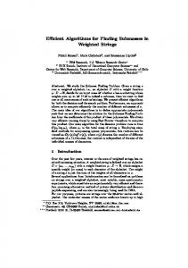
We have noticed in Section 2.3 that one can stop the hitting set algorithm at any time and use the size of the last hitting set H as a lower bound on the size of a critical subgraph. This is only true in the case where MinHS finds optimal solutions to the NP-hard minimum hitting set problem. We now present another algorithm for computing a lower bound on the size of critical subgraphs Given a graph G, an integer k and an integer imax , the lower bound algorithm computes a lower bound on the size of a k-VCS or k-ECS, using no more than imax iterations. This algorithm uses a function µ : S → N+ that associates to each vertex or edge s ∈ S the number µ(s) of iterations i where this vertex or edge was in the set U (ci ). In other words, µ(s) is initially equal to 0 for all s ∈ S, and at each iteration i, Min returns a coloring ci and µ(s) is incremented by one unit for each s ∈ U (ci ). A temporary lower bound b′ is then obtained from a function g defined below. Definition Let s1 ≥ . . . ≥ s|S| be an ordering of the elements in S such that µ(s1 ) ≥ . . . ≥ µ(s|S| ). Given an integer i, g(µ, i) is defined as the smallest integer l such that Pl j=1 µ(sj ) ≥ i Finally, since the lower bound b′ given by g can decrease from one iteration to another, the best lower bound b is set equal to the greatest value between the previous best value b and the new bound b′ . To illustrate the lower bound algorithm, consider once again the graph in Figure 3, which contains one minimum 3-ECS that the insertion algorithm fails to detect. Figure 5 shows the details of the first seven iterations of the algorithm. As before, the first 2coloring c1 has a set U (c1 ) containing the three edges forming a triangle in the center of the graph. For those edges e, µ(e) is increased to 1, w(e) is set equal to |S|, and since only

Les Cahiers du GERAD

12

G–2004–31

Algorithm 5 lower bound Input: A graph G, an integer k and an integer imax ; Output: A lower bound b. Initialization for all s ∈ S do µ(s) ← 0; end for i ← 0; Computation while i < imax do for all s ∈ S do w(s) ← |S|µ(s) ; end for c ← Min(G, k − 1, w); for all s ∈ U (c) do µ(s) ← µ(s) + 1; end for
b = max b, g(µ, i) ; end while

b=1 i=2

b=1 i=1

b=2 i=5 µ(e)=1

b=2 i=3

b=2 i=6 µ(e)=2

b=2 i=4

b=3 i=7 µ(e)=3

µ(e)=4

Figure 5: Illustration of the minimum size lower bound algorithm

Les Cahiers du GERAD

G–2004–31

13

one of them is required to total i = 1, the lower bound b is set to 1. The next 2-coloring c2 is such that U (c2 ) contains one of the three middle edges, and four other edges to cover all the remaining 3-ECSs, as shown in the second graph of Figure 5. Thus, the leftmost edge e of the triangle gets µ(e) = 2 and since this single value is sufficient to total i = 2, b remains equal to 1. The same happens for c3 , except that the rightmost edge is in U (c3 ) and that two edges are now required to total i = 3, and thus b = 2. Next, c4 has all three edges of the triangle with µ(e) = 2, and given that only two of those are required to total i = 4, b remains equal to 2. The fifth and sixth 2-colorings then cause two of the edges of the triangle to have µ(e) = 3 such that b still remains equal to 2. However, for the seventh 2-coloring, three edges are necessary to total i = 7, and the lower bound b therefore becomes 3. Because b then equals the size of the smallest 3-ECS, all subsequent iterations of this algorithm would be useless. Hence, imax = 7 is an optimal number of iterations for this particular graph. There are cases, however, where this algorithm fails to obtain a lower bound equal to the size of a minimum critical subgraph. For example, consider the graph in Figure 6 which has a chromatic number of 4. Given the task of finding a lower bound to the minimum 3-VCS, one can verify that the algorithm returns a lower bound of 2, while any triangle in this graph is a 3-VCS of size 3.

Figure 6: A graph producing a sub-optimal minimum size lower bound

7

Computational experiments

In this section we present some computational experiments related to the algorithms described in the previous sections. The purpose of these experiments is twofold: to analyze the pros and cons of each algorithm in finding critical subgraphs, and to evaluate the general benefit of finding critical subgraphs of a graph G for the computation of χ(G). All experiments were carried out on computers having a 1.6Ghz Athlon processor and 512Mb of RAM.

7.1

Implementation insights

When using heuristic implementations for procedure Min, the removal and insertion algorithms may produce errors. More precisely, it can happen that, based on the output of Min, vertices or edges are removed from G (i.e. their weight is set equal to 0) so that a subgraph H is obtained with χ(H) < k ≤ χ(G). In the case of the insertion algorithm, such errors can be detected if the output c of Min has value f (c) = 0. One can correct these errors by restoring the weight of previously removed vertices or edges to 1, until f (c) > 0. There are many ways to choose which removed vertex or edge to re-insert first.

Les Cahiers du GERAD

G–2004–31

14

One possibility, based on the fact that the error was probably committed at a recent iteration, is to re-insert them in the reverse order of their removal. Another possibility is to use the neighborhood weight heuristics (see Section 3) to select the vertex or edge that is the closest to those of weight |S|, thus trying to generate denser critical subgraphs. A similar strategy can be implemented to detect errors in the removal algorithm. When errors are detected and repaired, it may happen that the subgraph H produced by the removal or insertion algorithm is not critical (especially if the repairing strategy does not re-insert vertices or edges in the reverse order of their removal). Hence, if desired, one can re-apply the critical subgraph detection algorithm on H, and repeat this process until no additional vertex or edge can be removed.

7.2

Experimental data

The experiments were carried out on two sets of instances. The first set contains (n, p) random graphs. Given a positive integer n and a real number p ∈ [0, 1], the corresponding (n, p) random graph is such that |V | = n and all n(n − 1)/2 ordered pairs of vertices have a probability p of being linked by an edge in E. Parameter p is called the edge density of the graph. As a convention, we give the name “Rhni.hpi” to a particular (n, p) random graphs generated in our experiments. The second set of instances used for the experiments are the DIMACS benchmark graphs, which come from various sources. For a detailed description of these instances, the reader can refer to [13] or http://mat.gsia.cmu.edu/COLOR04.

7.3

VCS versus ECS detection

The first experiment aims at comparing VCS and ECS detection on a (50, 0.5) random graph R50.5 that has 590 edges and a chromatic number of 9. Table 1 shows the results of critical subgraph detection on R50.5 using three algorithms: the removal algorithm with neighborhood weight heuristic (Rem+h), the insertion algorithm also with neighborhood weight heuristic (Ins+h), and the pre-filtering algorithm followed by Ins+h (Filter+Ins). For each of these detection algorithms, 10 k-VCSs and 10 k-ECSs were found for k = 9, using different random seeds for Min. The average number of vertices and edges of these critical subgraphs is shown under the columns labeled |V ′ | and |E ′ |, and the resulting average edge densities under the column labeled p′ . The chromatic number of these subgraphs was then obtained using an exact coloring algorithm based on the one described in [18], after an average number of backtracks shown in the column labeled btk′ . From these results, we can see that the detection algorithms perform differently on VCSs than on ECSs. For instance, Filter+Ins produces, on average, the smallest VCSs of the three algorithms, but yields the biggest ECSs. On the other hand, Rem+h produces, on average, the biggest VCSs of the three algorithms, while smallest ECSs are obtained by the same algorithm. Differences also emerge between the VCSs and ECSs found by the detection algorithms. While ECSs have fewer edges than VCSs, VCSs tend to have less vertices. Consequently, the edge density of ECSs is much less than that of VCSs (0.44 on average for ECSs compared to 0.54 for VCSs). Notice also that the edge density of VCSs is greater than the expected 0.5. This increase is probably due to the use of the neighborhood

Les Cahiers du GERAD

15

G–2004–31

weight heuristic and pre-filtering algorithm that help finding denser subgraphs. A less predictable result is the huge difference in the number of backtracks required for VCSs and ECSs (367 on average for VCSs compared to 1670 for ECSs). This gap can mostly be explained by the difference in edge density of the subgraphs. Firstly, VCSs have fewer vertices resulting in a smaller search space for the exact coloring algorithm. Secondly, the greater number of edges in VCSs results in more constraints to eliminate illegal colorings from the search space, thus reducing the number of backtracks. When the goal is to find a lower bound on χ(G), we have observed that it is more efficient to search for VCSs than ECSs. Apart from producing critical subgraphs that are easier for the exact coloring algorithm to solve, VCS detection requires a lesser number of iterations than ECS detection. In the case of the removal algorithm, the number of iterations required to find a critical subgraph, which estimates the calculation time complexity, is, in the worst case, equal to |V | for VCS detection, and |E| for ECS detection. For the insertion algorithm, the number of iterations is, in the worst case, equal to the size of H. For example, VCS detection on R50.5 using Ins+h took, on average, 37 iterations while 345 iterations were required for ECSs detection using the same algorithm. For these reasons, the next experiments focus on VCS detection. Method Rem+h Ins+h Filter+Ins

|V ′ | 38.2 37.1 36.3

VCS |E ′ | p′ 384.1 0.54 355.7 0.53 344.7 0.54

btk′ 380.4 348.5 371.8

|V ′ | 36.8 41.2 41.9

ECS |E ′ | p′ 327.5 0.50 344.8 0.42 344.4 0.40

btk′ 1089.4 1295.4 2625.4

Table 1: Vertex-critical and edge-critical subgraph detection on graph R50.5

7.4

VCS detection by hitting set algorithm

The next experiment evaluates the hitting set algorithm. We have generated a (n, 0.5) random graph for each n ∈ {15, 20, 25, 30, 35, 40, 45, 50}. For each such graph G, we have applied the hitting set algorithm 10 times for the detection of k-VCSs with k = χ(G), each time using different random seeds for Min and MinHS. The values χ(G) were obtained by means of the exact coloring algorithm. Table 2 shows the number of vertices |V | and edges |E| of these random graphs, and their chromatic number χ(G). The column labeled |V ′ | contains the average number of vertices of the detected k-VCSs, and the column labeled iter indicates the average number of iterations that this algorithm took to find the corresponding subgraphs. A tabu search implementation for MinHS was used. Thus, unless the k-VCS is a clique, we have no guarantee that it is minimum. |V | 15 20 25

Graph |E| χ(G) 46 4 90 5 137 6

VCS |V ′ | iter 4 10.9 5 16.6 9 40.4

. . . continued on next page

Les Cahiers du GERAD

G–2004–31

|V | 30 35 40 45 50

Graph |E| χ(G) 211 7 277 7 369 8 473 9 590 9

|V ′ | 7 7 25 42 32

16

VCS iter. 22.2 41.7 641.5 164.8 2554.4

Table 2: Hitting set algorithm on 0.5 density random graphs The results presented in Table 2 show that the hitting set algorithm found, for all instances, 10 subgraphs having the same |V ′ |, which indicates that these critical subgraphs are most probably minimum. Most importantly, these results reveal that the number of iterations of the hitting set algorithm is, as predicted, exponential on |V |. Notice, however, that this relation is not strictly increasing, as the number of iterations shortly drops when χ(G) increases. This phenomenon is detailed in an experiment presented later in this paper (see Section 7.6).

7.5

Detection heuristics and lower bounds comparison

The next experiment has two goals. The first goal is to analyze the impact of using the neighborhood weight heuristic and the pre-filtering algorithm on VCS detection. The second goal is to compare the lower bounds on the size of a VCS obtained by the hitting set algorithm and by the lower bound algorithm presented in section 6. Table 3 contains the results of this experiment. The first four columns of this table contain the name, number of vertices and edges, as well as the chromatic number of the instances used in the experiment. The next five columns contain the minimum, median and maximum number of vertices of 10 k-VCSs for k = χ(G), found by five detection algorithms, each time using a different random seed for Min: the removal algorithm without any heuristic (Rem), the removal algorithm with the neighborhood weight heuristic (Rem+h), the insertion algorithm without any heuristic (Ins), the insertion algorithm with the neighborhood weight heuristic (Ins+h), and the pre-filtering algorithm followed by Ins+h (Filter+Ins). Finally, the last two columns show the minimum, median and maximum number of vertices of the k-VCSs detected for k = χ(G) by the hitting set algorithm (HS ) and the minimum, median and maximun values produced by the lower bound algorithm (LB ). For HS, the values preceded by “≥” represent lower bounds obtained when stopping the hitting set algorithm after 3000 iterations. The results in Table 3 clearly indicate that the removal and insertion algorithms perform better when combined with the neighborhood weight heuristic. In all but one case (Rem on queen6 6 ), the smallest VCSs found using the heuristic have a lesser or equal number of vertices than the ones found without any heuristic. More importantly, the median number of vertices of VCSs found with the heuristic is strictly smaller for all instances except one (again Rem on queen6 6 ), while the biggest VCSs found using the neighborhood weight heuristic have fewer vertices for all instances. Thus, the neighborhood weight heuristic also reduces the variance in the size of critical subgraphs found. A good example is DSJC125.1

Les Cahiers du GERAD

G–2004–31

17

which contains minimum VCSs of only 10 vertices. The simple removal algorithm found such minimum subgraphs in 2 out of 10 cases, whereas the same algorithm using the neighborhood weight heuristic found one in 6 cases. Furthermore, the biggest VCS found using Rem+h has only 13 vertices, compared to 50 for Rem. Algorithm Filter+Ins seems to perform even better as a heuristic to find smaller VCSs. For the R50.5, R60.5, queen6 6 and queen8 8 instances, Filter+Ins finds VCSs containing fewer vertices than those found by any other detection algorithm. Moreover, for the R50.5 and queen6 6 instances, these subgraphs were shown minimum by the hitting set algorithm. Considering that Filter+Ins is usually faster than the other detection algorithms, it is probably the best algorithm to find critical subgraphs. Graph name |V | |E| χ R50.5 50 590 9 R60.5 60 858 10 DSJC125.1 125 736 5 queen6 6 36 290 7 queen8 8 64 728 9 queen9 9 81 2112 10

Rem |V ′ | 36,41,44 48,51,53 10,31,50 25,27,29 57,58,59 -

Rem+h |V ′ | 36,38,41 44,46,48 10,10,13 26,27,27 54,55,56 73,74,74

Ins |V ′ | 37,41,44 49,52,54 68,84,87 27,28,30 56,58,60 -

VCS Ins+h Filter+Ins HS LB |V ′ | |V ′ | |V ′ | |V ′ | 34,37,39 32,36,40 32,32,32 13,13,13 45,46,48 43,44,46 ≥ 36 10,10,11 10,14,53 11,14,35 ≥ 10 4,4,5 24,27,28 22,24,27 22,22,22 7,7,7 54,55,56 53,55,56 ≥ 29 11,11,12 73,74,75 73,75,76 - 12,12,13

Table 3: Detection heuristics impact and lower bounds of vertex-critical subgraph As for finding lower bounds on the size of minimum VCSs, the last two columns of Table 3 show that HS performs better than LB. For all instances tested with HS, the lower bounds found had more vertices than those found with LB. For example, HS found a lower bound of 36 vertices for R60.5, while LB produced a best lower bound of 11 vertices. Moreover, HS found actual minimum VCSs for R50.5 and queen6 6. In brief, when the size of the instance allows its use, HS yields better lower bounds than LB.

7.6

VCS detection on random graphs

The next experiment focuses on finding VCSs in random graphs for the computation of their chromatic number. Because they have no particular structure, (n, p) random graphs are probably the least suitable instances for finding critical subgraphs. Depending on the edge density p, such graphs can contain critical subgraphs that have almost as many vertices or edges as the original graph. Tables 4 and 5 show the results of VCS detection for random graphs of edge density 0.1 and 0.5. We have generated four different random graphs for each pair (n, 0.1) with n ∈ {100, 110, . . . , 220}, and for each pair (n, 0.5) with n ∈ {80, 90, 95, 100}. The first four columns contain the number of vertices and edges of the instances, an upper bound k for χ(G), and the number of backtracks required by the exact coloring algorithm to determine χ(G). Backtrack values given without parentheses indicate that we have been able to compute χ(G) and, in such a case, we have fixed k = χ(G). However, backtrack values enclosed in parentheses mean that we have not been able to compute χ(G) and we

Les Cahiers du GERAD

18

G–2004–31

indicate the CPU-time (in seconds) it took for the exact coloring algorithm to exceed the maximum allowed number of backtracks (250000000). In such a case, k can be strictly larger than χ(G). Graph |V | 100 100 100 100 110 110 110 110 120 120 120 120 130 130 130 130 140 140 140 140 150 150 150 150 160 160 160 160 170 170 170 170 180 180 180 180 190 190

|E| 496 447 499 507 600 555 592 610 715 669 714 706 795 832 828 843 972 936 988 968 1103 1098 1120 1128 1261 1251 1274 1279 1430 1414 1460 1440 1603 1617 1584 1639 1799 1784

k btk |V ′ | 5 92 38 5 193 66 5 33 38 5 135 46 5 114 34 5 45 36 5 131 33 5 72 43 5 7105 32 5 45 21 5 1172 31 5 186 27 5 173090 31 5 62743 34 6 1519301 113 6 462073 100 6 767916 99 6 1130903 103 6 138308 83 6 906265 105 6 829224 96 6 109821 93 6 79497 81 6 194667 91 6 187661 87 6 101953 83 6 107938 79 6 199720 87 6 (43603) 80 6 8320828 80 6 (45118) 69 6 70336660 85 6 (46199) 78 7 (44611) 158 7 (45690) 168 7 (43834) 148 7 (49624) 147 7 (47708) 152

Rem+h |E ′ | btk′ |V ′ | 137 109 55 263 233 62 137 63 44 175 105 51 119 32 61 126 40 50 116 58 46 162 117 51 113 59 52 63 10 38 109 67 50 88 71 61 108 30 42 120 47 46 712 1493884 112 617 415567 101 625 1551179 102 640 1610227 107 499 137685 94 654 4436370 108 610 1289371 99 579 247208 95 481 133880 87 554 115757 98 539 347890 103 501 140258 95 474 71615 91 529 250846 103 487 168991 97 477 85597 96 405 7660 80 516 193161 96 467 10347 102 1386 (41491) 159 1471 (45480) 168 1278 (37592) 148 1281 (39683) 156 1327 (41621) 157

VCS Ins+h |E ′ | btk′ |V ′ | 207 271 38 234 333 63 160 66 42 198 151 42 244 201 41 188 98 36 170 330 33 188 57 43 199 157 42 134 16 33 195 38 36 239 693 43 150 87 35 171 59 42 702 1898057 113 617 519210 99 637 1122434 99 664 1439572 104 569 202552 88 681 1621338 104 622 887587 97 581 148611 93 517 234917 88 606 112071 98 642 407695 94 580 126134 92 536 148744 83 647 7955344 93 597 340743 89 581 490732 85 470 7367 73 581 61871 93 613 294620 87 1386 (42298) 158 1467 (45627) 168 1266 (39431) 150 1359 (41245) 152 1352 (43114) 154

Filter+Ins |E ′ | btk′ 138 122 242 282 156 55 151 237 151 116 123 97 113 30 157 76 156 31 108 32 126 121 157 102 115 39 154 41 710 2094563 605 323833 615 970417 647 2775637 522 149205 643 3149618 606 1164246 565 202147 531 274521 591 298509 582 520562 561 96891 497 81926 564 257126 550 167544 500 94995 421 10720 563 207389 519 44426 1389 (41474) 1467 (45627) 1286 (39265) 1327 (41473) 1337 (41929)

. . . continued on next page

Les Cahiers du GERAD Graph |V | 190 190 200 200 200 200 210 210 210 210 220 220 220 220

|E| 1826 1785 2036 1941 2026 1977 2221 2123 2226 2175 2422 2348 2435 2387

k 7 7 7 7 7 7 7 7 7 7 7 7 7 7

btk |V ′ | (49295) 140 (49653) 158 (50830) 139 (48910) 153 (46221) 130 (47076) 146 (61537) 134 (54287) 146 (64066) 129 (59757) 139 (62081) 132 (59384) 137 (56396) 125 (58686) 135

19

G–2004–31

Rem+h |E ′ | btk′ |V ′ | 1206 (38256) 152 1389 (44149) 160 1220 (46450) 147 1343 (63880) 155 1113 (44259) 150 1278 (46846) 147 1166 (34091) 148 1277 (38301) 157 1109 (33831) 143 1210 (36732) 153 1145 (32986) 148 1188 (34917) 149 1070 (31717) 146 1166 (34208) 145

VCS Ins+h |E ′ | btk′ |V ′ | 1307 (40572) 141 1403 (43280) 160 1291 (46855) 148 1347 (64474) 155 1288 (60526) 148 1281 (47080) 152 1289 (37564) 144 1367 (39882) 154 1213 (35316) 136 1331 (38900) 149 1279 (37429) 139 1290 (37488) 148 1259 (37417) 134 1241 (34873) 144

Filter+Ins |E ′ | btk′ 1206 (38298) 1405 (44872) 1281 (45411) 1347 (63452) 1277 (47730) 1324 (48111) 1256 (37077) 1342 (40706) 1161 (35703) 1283 (38497) 1208 (35358) 1281 (36713) 1144 (34620) 1245 (35136)

Table 4: Vertex-critical subgraph detection on 0.1 density random graphs Graph |V | 80 80 80 80 90 90 90 90 95 95 95 95 100 100 100 100

|E| 1547 1528 1609 1582 1924 1984 1978 2003 2223 2149 2223 2208 2381 2444 2469 2465

k btk |V ′ | 12 14029599 64 12 12860059 59 13 7255750 75 13 58684771 75 13 128822599 74 13 133509732 72 14 (26310) 88 14 (26271) 86 14 (28823) 82 14 (27836) 89 14 (28861) 83 14 (28553) 85 14 (30027) 83 14 (30107) 81 15 (30328) 97 15 (31121) 100

Rem+h |E ′ | btk′ |V ′ | 1051 1285350 66 911 293100 60 1440 21670437 73 1425 22694200 74 1398 17898027 75 1354 4320820 73 1908 (26010) 87 1858 (25914) 84 1723 (27079) 83 1931 (26961) 89 1777 (27784) 88 1834 (26831) 84 1748 (25375) 87 1690 (26861) 85 2345 (28932) 96 2465 (29744) 99

VCS Ins+h |E ′ | btk′ |V ′ | 1086 3887945 63 926 531284 58 1380 6590146 72 1389 14340999 73 1402 30015939 71 1374 7693584 72 1870 (26268) 87 1783 (25912) 84 1754 (27116) 82 1935 (26994) 88 1906 (26981) 84 1780 (34611) 86 1869 (25959) 83 1828 (25663) 82 2297 (28595) 97 2425 (29499) 99

Filter+Ins |E ′ | btk′ 1007 726965 884 429381 1343 6387828 1350 20529374 1288 17201820 1334 11737502 1870 (26253) 1783 (26381) 1703 (26512) 1896 (27510) 1797 (27024) 1841 (26097) 1724 (26025) 1711 (25304) 2342 (28454) 2414 (29335)

Table 5: Vertex-critical subgraph detection on 0.5 density random graphs We have applied each algorithm 10 times on each instance, every time using a different random seed for Min. The other columns of Tables 4 and 5 contain the number of vertices and edges of the smallest k-VCS obtained by Rem+h, Ins+h and Filter+Ins for each instance, as well as the number of backtracks required to determine the chromatic number of these k-VCSs. Once more, backtrack values enclosed in parentheses indicates that the chromatic number of the corresponding subgraphs could not be determined by the exact coloring algorithm, and can be strictly smaller than k.

Les Cahiers du GERAD

20

G–2004–31

0.70

0.60 k=5 k=6 k=7

Vertex reduction

0.50

0.40

0.30

0.20

0.10

0.00 90

100

110

120

130

140

150

160

170

180

190

200

210

220

230

Original number of vertices

Figure 7: Vertex reduction of (n, 0.1) random graphs versus n Figures 7 and 8 were produced using the VCSs obtained by Filter+Ins 1 . Each curve contains instances for a particular value of k, and are drawn such that abscissa values are the number of vertices |V | of these instances, and ordinate values are the minimum, average and maximum reductions of vertices for the corresponding critical subgraphs. Given a critical subgraph of |V ′ | vertices, the vertex reduction is calculated as follows: |V | − |V ′ | |V | These figures first show that the vertex reduction decreases as p increases. Thus, the maximum vertex reduction reached for instances of 100 vertices is 62% when p = 0.1, whereas the maximum reduction for p = 0.5 is only 18%. This result comes as no surprise, since denser instances tend to have larger critical subgraphs. Furthermore, these figures reveal two opposite trends when considered separately. On the one hand, the vertex reduction decreases as k increases. Consider, for example, the reduction values for the curves in Figure 7. For k = 5, the maximum vertex reduction is 73%, while this value drops to 57% for k = 6, and 39% for k = 7. The same goes for the curves in Figure 8, where the maximum vertex reduction is 21% for k = 13, 18% for k = 14, and 3% for k = 15. On the other hand, the vertex reduction increases with n, for a particular value of k. Consider once more Figure 7. For k = 5, the maximum vertex reduction increases from 62%, when n = 100, to a higher 73%, for n = 130. Likewise, for k = 6 the reduction rises from 24%, for n = 130 to 57% for n = 170. Finally, the same happens for k = 7, where the reduction increases from 7% to 38% as n varies from 180 to 220. 1

The VCSs found using Rem+h and Ins+h produce similar curves.

Les Cahiers du GERAD

21

G–2004–31

0.25

Vertex reduction

0.20

0.15 k = 13 k = 14 k = 15

0.10

0.05

0.00 75

80

85

90

95

100

105

Original number of vertices

Figure 8: Vertex reduction of (n, 0.5) random graphs versus n 1.20

1.00

0.80

0.60

Backt ra ck reduc tion

k= 5 k= 6 0.40

0.20

0.00

-0.2 0

-0.4 0

-0.6 0 90

100

110

120

130

140

15 0

1 60

17 0

1 80

Original num ber of ve rtices

Figure 9: Back reduction of (n, 0.1) random graphs versus n

Les Cahiers du GERAD

G–2004–31

22

Figure 9 shows the maximum backtrack reduction for the k-VCSs obtained with a particular value of k. Consider the backtrack reduction curve for k = 5. For n = 100, the maximum backtrack reduction is −33% (i.e. the number of backtracks actually increases). However, the maximum backtrack reduction rises to an excellent 77% for n = 110, and almost 100% for n = 120 and n = 130. For k = 6, the maximum backtrack reduction starts off at a positive 30% for n = 130, but then drops to −8% for n = 140 and a low −40% for n = 150. Fortunately, the maximum reduction increases again to a positive 24% for n = 160 and reaches close to 100% for n = 170 and n = 180. These results suggest that searching for critical subgraphs is especially useful for instances having as many vertices as possible for a particular χ(G). In most combinatorial problems, there is a very sharp transition between instances that can be solved optimally and those that cannot. In the case of random graphs of edge density 0.1, the exact coloring algorithm used in this experiment solved all instances of 160 vertices with less than 200000 backtracks, while two out of four instances of 170 vertices were not solved after 250000000 backtracks, and none of the instances of 180 vertices were solved within the same limit. However, these instances are close to the maximum number of vertices for k = 6, and are thus excellent candidates for the critical subgraph detection. In fact, the two instances of 170 vertices that were not solved within limits produced critical subgraphs that were easily solved in 167544 and 7367 backtracks, and the one instance of 180 vertices for k = 6 gave a critical subgraph that was solved in only 10347 backtracks. As a final observation, the results of this experiment reveal a surprising phenomenon. As the number of vertices of a given instance is reduced, one can expect the exact coloring algorithm, which has a computational complexity exponential in the number of vertices, to solve that instance in a lesser or equal number of backtracks. However, Figure 9 shows that this is not always the case. For example, for instances of 150 vertices, all the critical subgraphs found increased the number of backtracks instead of reducing it. A more striking example is a critical subgraph found by Ins+h that reduced the number of vertices from 160 to 103. While the original instance took 199720 backtracks to solve, this critical subgraph was solved after as much as 7955344 backtracks (3883% increase). This phenomenon, was previously observed by Herrmann and Hertz in [11].

7.7

VCS detection on benchmarks

The last experiment, which results are presented in Table 6, deals with DIMACS benchmark graphs. The purpose of this experiment is to find VCSs in these instances in order to compute a lower bound on their chromatic number. The first four columns in Table 6 contain the names of the instances, their number of vertices and edges, as well as the number of backtracks needed by the exact coloring algorithm to determine χ(G). Backtrack values enclosed in parentheses represent the number of backtracks made by the exact coloring algorithm after reaching a 4 hour CPU-time limit. In such a case, no value was obtained for χ(G). The next column contains a lower bound k on χ(G). Values of k preceded by an asterisk “∗” indicate that χ(G) is known, and that k = χ(G). The following three columns contain the number of vertices and edges of the smallest k-VCSs, found within

Les Cahiers du GERAD

23

G–2004–31

five attempts using a different random seed for Min, and the number of backtracks required by the exact coloring algorithm to determine the chromatic number of these subgraphs. Once again, values enclosed in parentheses indicate that this chromatic number was not determined within the same CPU-time limit, and might be different from k. Finally, the last column contains lower bounds on the size of k-VCSs obtained by means of the lower bound algorithm. name myciel3 myciel4 myciel5 myciel6 myciel7 mug88 1 mug88 25 mug100 1 mug100 25 1-Insertions 1-Insertions 1-Insertions 2-Insertions 2-Insertions 2-Insertions 3-Insertions 3-Insertions 3-Insertions 4-Insertions 4-Insertions fpsol2.i.1 fpsol2.i.2 fpsol2.i.3 inithx.i.1 inithx.i.2 inithx.i.3 mulsol.i.1 mulsol.i.2 mulsol.i.3 mulsol.i.4 mulsol.i.5 zeroin.i.1 zeroin.i.2

4 5 6 3 4 5 3 4 5 3 4

|V | 11 23 47 95 191 88 88 100 100 67 202 607 37 149 597 56 281 1406 79 475 496 451 425 864 645 621 197 188 184 185 186 211 211

Graph |E| 20 71 236 755 2360 146 146 166 166 232 1227 6337 72 541 3936 110 1046 9695 156 1795 11654 8691 8688 18707 13979 13969 3925 3885 3916 3946 3973 4100 3541

btk 4 106 30998 (138446852) (77223695) 2204467 942961 1406570 974170 104296036 (133727661) (50929137) 3064 (154902785) (48458541) 723616 (95076991) (13784327) (228367528) (70891706) (169107715) 2 2 1 (139157853) (141407783) 1 6 6 (161605284) (161214648) 24 11472

VCS k |V ′ | |E ′ | btk′ *4 11 20 *5 23 71 *6 47 236 *7 95 755 *8 191 2630 *4 88 146 *4 88 146 *4 100 166 *4 100 166 *5 67 232 6 202 1227 7 607 6337 *4 37 72 *4 37 72 6 597 3936 *4 56 110 5 281 1046 6 1406 9695 *3 13 13 5 475 1795 *65 65 2080 0 *30 30 435 0 *30 30 435 0 *54 54 1431 0 *31 31 465 0 *31 31 465 0 *49 49 1176 0 *31 31 465 0 *31 31 465 0 *31 31 465 0 *31 31 465 0 *49 49 1176 0 *30 30 435 0 . . . continued on next

LB 11 23 47 95 189 55 56 67 68 67 202 448 37 14 208 56 220 73 6 232 24 24 24 41 25 25 44 24 25 24 28 44 27 page

Les Cahiers du GERAD

name zeroin.i.3 le450 15a le450 15b le450 15c le450 15d le450 25a le450 25b le450 25c le450 25d le450 5a le450 5b le450 5c le450 5d school1 school1 nsh anna david homer huck jean games120 miles1000 miles1500 miles250 miles500 miles750 DSJC125.1 DSJC125.5 DSJC125.9 DSJC250.1 DSJC250.9 DSJR500.1 DSJR500.1c DSJR500.5 queen5 5 queen6 6 queen7 7 queen8 12 queen8 8 queen9 9

G–2004–31

Graph VCS |V | |E| btk k |V ′ | |E ′ | btk′ LB 206 3540 11472 *30 30 435 0 27 450 8168 (54447597) *15 15 105 0 7 450 8169 (49996287) *15 15 105 0 7 450 16680 (40481025) *15 15 105 0 3 450 16750 (35180270) *15 15 105 0 3 450 8260 14 *25 25 300 0 20 450 8263 12 *25 25 300 0 19 450 17343 (41188964) *25 25 300 0 7 450 17425 (42974825) *25 25 300 0 7 450 5714 (21467721) *5 5 10 0 2 450 5734 (28479480) *5 5 10 0 2 450 9803 5 *5 5 10 0 2 450 9757 5754158 *5 5 10 0 2 385 19095 17 *14 14 91 0 2 352 14612 (59393984) 14 14 91 0 2 138 493 8 *11 11 55 0 11 87 406 36 *11 11 55 0 11 561 1629 (244497375) *13 13 78 0 13 74 301 211680 *11 11 55 0 11 80 254 8645 *10 10 45 0 10 120 638 (516246020) *9 9 36 0 9 128 3216 4583894 *42 42 861 0 41 128 5198 1692256 *73 73 2628 0 73 128 387 (136594896) *8 8 28 0 8 128 1170 8 *20 20 190 0 20 128 2113 434 *31 31 465 0 28 125 736 227 *5 10 26 1 4 125 3891 (71844096) 14 80 1674 37453055 125 6961 (68250955) 40 78 2782 (205206643) 250 3218 (42398413) 6 70 410 3621 250 27897 (33839645) 50 133 8052 (88911252) 500 3555 (141520342) 12 12 66 0 11 500 121275 (6401403) 63 63 1953 0 2 500 58862 (73970922) 26 26 325 0 1 25 160 1 *5 5 10 0 5 36 290 410 *7 25 148 45 7 49 476 2555 *7 7 21 0 5 96 1368 (139081460) *12 12 66 0 11 64 728 597552 *9 54 538 188021 11 81 2112 80603809 *10 74 897 135083408 12 . . . continued on next page

24

Les Cahiers du GERAD

name queen10 10

|V | 100

queen11 11 121 queen12 12 144 queen13 13 169 queen14 14 196 queen15 15 225 queen16 16 256 ash331GPIA 662 1-FullIns 3 30 1-FullIns 4 93 1-FullIns 5 282 2-FullIns 3 52 2-FullIns 4 212 2-FullIns 5 852 3-FullIns 3 80 3-FullIns 4 405 3-FullIns 5 2030 4-FullIns 3 114 4-FullIns 4 690 5-FullIns 3 154

Table 6:

G–2004–31 Graph |E| btk 2940 (134401345) 3960 5192 6656 8372 10360 12640 4185 100 593 3247 201 1621 12201 346 3524 33751 541 6650 792

(116006580) (101315208) (90800757) (83679129) (69555352) (72473005) 14 7 5567 (106523508) 1850 (209999176) (91922086) 366830 (164058937) (34366333) 80247163 (126559559) (448858523)

25

VCS k |V ′ | |E ′ | btk′ LB 10 10 45 0 *11 89 1220 (424776367) 11 *11 11 55 0 6 *12 12 66 0 *13 13 78 0 6 *14 14 91 0 15 15 105 0 16 16 120 0 *4 9 16 2 2 *4 7 12 1 7 *5 15 43 6 14 *6 31 144 271 19 *5 9 22 1 9 *6 19 75 8 19 *7 39 244 715 31 *5 5 10 0 5 *7 23 116 10 23 *8 47 371 1675 *7 13 51 1 13 *8 27 166 12 25 *8 15 70 1 15

Vertex-critical subgraph detection on Color04 graphs

To facilitate the presentation of the results in Table 6, we will divide the instances in three categories. The first category is composed of instances that are probably vertexcritical for χ(G). Graphs having myciel, mug or Insertions in their name fall into this category. Results in Table 6 show that for the fourteen instances where k = χ(G) (i.e., there is an asterisk in the fifth column), we have got a proof that G is a vertex critical since V is the output of the detection algorithm. In the six other cases were k is possibly strictly smaller than χ(G), we have a proof that either k < χ(G) or G is vertex critical. Furthermore, because we used the speed-up technique in combination with the detection algorithm, these graphs were shown possibly critical after only a small number of iterations, even for those with a great number of vertices. For example, 3-Insertions 5 which has 1406 vertices, was shown possibly vertex-critical by Ins+h using the speed-up technique in only 22 iterations2 . The speed-up technique is thus highly useful for showing that a given graph is critical. As regards lower bounds on the size of VCSs, we found in most cases values close or equal to |V |. For example, we obtained a lower bound equal to |V | for all but one myciel graphs. The second category contains the instances which have cliques as minimum k-VCSs, for k = χ(G). The graphs anna, david, homer, huck, jean, as well as those having fpsol2, 2

As many as 1152 vertices of the critical subgraph were found after the first iteration, and 1372 after the second.

Les Cahiers du GERAD

G–2004–31

26

inithx, mulsol, zeroin, le450, school1, games120 or miles in their name are such instances. These instances are interesting because they have the smallest possible critical subgraphs (i.e., k-VCSs with k vertices) that are therefore easier to detect. Moreover, the chromatic number of a clique is equal to its number of vertices, such that the exact coloring algorithm is not required at all. From Table 6, we see that cliques were found as VCSs for all 39 instances in this category, among which 17 had not been solved by the exact coloring algorithm. Once more, the lower bound procedure gives decent results for instances in this second category. Finally, the last category is composed of all the instances falling in none of the two first categories. Among those are the DSJC instances, which are standard (n, p) random graphs used by Aragon et al. in [1]. As mentioned in the previous experiments, random graphs are generally poor candidates for the detection algorithms because, as opposed to instances in the second category, they have critical subgraphs of large size. Except for DSJC125.1, which has a 5-VCS of only 10 vertices, we therefore focused on the search of interesting lower bounds k ≤ χ(G) for these instances. We thus showed for DSJC125.5 that χ(G) ≥ 14, while, to our knowledge, the best known bound for this instance was 13. Additionally, we were able to show that χ ≥ 6 for DSJC250.1. However, the lower bound k one can obtain for a given instance is limited by the size of the k-VCSs that can be found for this instance. Thus, even though we were able to find a k-VCS for DSJC250.9 for k = 50, this subgraph was too big (133 vertices and 8052 edges) for the exact coloring algorithm to determine its chromatic number. The queenN N graphs are also comprised in this last category of instances. These graphs are particular because the minimum k-VCSs for k = χ(G) are either cliques3 or subgraphs containing most of the vertices of the original instance. Accordingly, we were able to find k-VCSs for k = χ(G) when these subgraphs were cliques (i.e., queen5 5, queen7 7, queen8 12, queen11 11, queen12 12, queen13 13 and queen14 14 ). We were also able to compute χ(G) for queen6 6, queen8 8 and queen9 9 after finding k-VCSs that are small enough to be solved by the exact coloring algorithm. Finally, we only achieved a lower bound of k = N for queen10 10, queen15 15 and queen16 16. The last set of instances in this category are the FullIns graphs, which were built by adding extra nodes to critical graphs. These instances are therefore perfect candidates for critical subgraph detection. To our knowledge, the chromatic number of all theses instances was known except for 2-FullIns 4, 2-FullIns 5, 3-FullIns 4 and 4-FullIns 4. For these four graphs, we were able to raise the best known lower bound to equal the best known upper bound, thus fixing the chromatic number. We have found, for k = χ(G), k-VCSs in all these instances and could easily compute the chromatic number of these critical subgraphs using an exact coloring algorithm. Notice that when applied on the original graph, the exact coloring algorithm could only determine the chromatic number of 5 of these instances. 3

This is always the case for odd values of N that are not multiple of 3.

Les Cahiers du GERAD

G–2004–31

27

To finish, the bounds obtained for this category of instances are much lower than the number of vertices of the critical subgraphs found. Knowing that these instances most probably have large minimum critical subgraphs, we come to the conclusion that LB gives poor results for this category of instances.

7.8

Calculation time of detection algorithms

Since procedure Min accounts for almost all of the calculation complexity of the critical subgraph detection algorithms4 the total CPU-time mainly depends on the number of time this procedures is called (i.e. number of iterations), as well as on the time spent on each call. We have implemented procedure Min using a tabu search procedure (see Section 4). If the tabu search is stopped too early, its output is possibly not optimal, and this induces errors that have to be repaired. On the other hand, if the tabu search is run for a very long time, the detection algorithms, in turn, will take a lot of time to complete their task. Instead of defining a general stopping criteria that works reasonably well on all instances, we found easier tuning the tabu search for each instance. Moreover, since our aim is not to design the fastest possible critical subgraph detection algorithm, a small amount of time has been spent on this tuning. Here are some general indications on the total time needed to detect critical subgraphs using our tuning. The detection of VCSs for the instances in Tables 4 and 5, using the removal and insertion algorithms, took a few seconds for the smaller instances up to a few hours for the bigger ones. Furthermore, the pre-filtering algorithm helped, in most cases, to lower the calculation time for the bigger instances to under an hour. Notice however, these instances were the worst encountered during experimentation. Indeed, the detection algorithms on critical benchmark graphs took only a few seconds, using the speed-up technique. In addition, the detection algorithms generally took a few minutes for instances which have cliques as minimum critical subgraphs. Finally, the time needed to obtain lower bounds on the size of critical subgraphs, using the hitting set algorithm and the lower bound algorithm, depends on the quality sought for these bounds. In the case of the hitting set algorithm, an hour is usually enough to produce a good bound, while a few minutes is sufficient for the latter algorithm.

8

Conclusion

We have presented algorithms to find vertex-critical and edge-critical subgraphs of a given graph. We have also described algorithms to find minimum critical subgraphs, as well as lower bounds on the size of these subgraphs. In addition, we have shown that such critical subgraphs could be used to find a lower bound on χ(G). Furthermore, because these algorithms need to solve the NP-hard k-coloring problem, we have indicated how heuristic algorithms for this problem can be used within the detection algorithms. Finally, we have presented various strategies to accelerate the detection algorithms, to find smaller critical subgraphs, and to correct errors that may occur because of the use of heuristic algorithms. 4

Except for the hitting set algorithm which also uses MinHS.

Les Cahiers du GERAD

G–2004–31

28

Experiments were carried out on different types of instances to evaluate the detection algorithms and to find lower bounds on the chromatic number. Those experiments have shown that some detection algorithms are more efficient than others. For example, we saw that the pre-filtering algorithm significantly reduces the number of iterations for the detection algorithms, and serves as a good heuristic to find small critical subgraphs. Furthermore, these experiments made it possible to identify on which instances the detection algorithms perform best. Using these results, we were able to improve known lower bounds on χ(G) for some instances, and even to compute the chromatic number of instances for which only bounds were known.

References [1]

[2] [3] [4]

[5] [6] [7] [8] [9] [10] [11] [12] [13]

[14] [15]

Aragon, C.R., Johnson, D.S., Mcgeoch, L.A., Schevon, C., Optimization by Simulated Annealing: an Experimental Evaluation. Part II, Graph Coloring and Number Partitioning, Operations Research 39, 1991, 378-406 Brown, J.R., Chromatic Scheduling and the Chromatic Number Problem, Management Science 19/4, 1972, 456-463 Chinneck, J.W., Finding a Useful Subset of Constraints for Analysis in an Infeasible Linear Program, INFORMS Journal on Computing 9/2, 1997 Chinneck, J.W., Feasibility and Viability, Advances in Sensitivity Analysis and Parametric Programming, T. Gal and H.J. Greenberg (eds.), Kluwer Academic Publishers, International Series in Operations Research and Management Science 6, 1997 Fleurent, C., Ferland, J.A., Genetic and Hybrid Algorithms for Graph Coloring, Annals of Operations Research 63, 1996, 437-461 Galinier, P., Hao, J.K., Hybrid Evolutionary Algorithms for Graph Coloring, Journal of Combinatorial Optimization 3/4, 1999, 379-397 Galinier, P., Hertz, A., Solution Techniques for the Large Set Covering Problem, Research Report G-2003-44, Les Cahiers du GERAD, Montr´eal, Canada, 2003 Garey, M.R., Johnson, D.S., Computers and Intractability : A Guide to the Theory of NPCompleteness, W.H. Freman and Company, NY, 1979 Glover, F., Tabu Search - part I, ORSA Journal on Computing 1/3, 1989, 190-206 Glover, F., Tabu Search - part II, ORSA Journal on Computing 2/1, 1989, 4-32 Herrmann, F., Hertz, A., Finding the Chromatic Number by Means of Critical Graphs, ACM Journal of Experimental Algorithmics 7/10, 2002, 1-9 Hertz, A., de Werra, D., Using Tabu Search for Graph Coloring, Computing 39, 1987, 345-351 Johnson, D.S., Trick, M.A., Proceedings of the 2nd DIMACS Implementation Challenge, DIMACS Series in Discrete Mathematics and Theoretical Computer Science 26, American Mathematical Society, 1996 Kubale, M., Jackowski, B., A Generalized Implicit Enumeration Algorithm for Graph Coloring, Communications of the ACM 28/4, 1985, 412-418 Mackworth, A.K., Constraint Satisfaction, S.C. Shapiro (Ed.) Encyclopedia on Artificial Intelligence, John Wiley & Sons, NY, 1987

Les Cahiers du GERAD

G–2004–31

29

[16] Mehrotra, A., Trick, M.A., A Column Generation Approach for Exact Graph Coloring, INFORMS Journal on Computing 8, 1996, 344-354 [17] Morgenstern, C., Distributed Coloration Neighborhood Search, D.S. Johnson and M.A. Trick, eds. Cliques, Coloring and Satisfiability: Second DIMACS Implementation Challenge. DIMACS Series in Discrete Mathematics and Theoretical Computer Science, American Mathematical Society 26, 1996, 335-357 [18] Peem¨ oller, J., A Correction to Br´elaz’s Modification of Brown’s Coloring Algorithm, Communications of the ACM 26/8, 1983, 593-597 [19] Tsang, E., Foundations of Constraint Satisfaction, Academic Press, London, 1993 [19] Van Loon, J., Irreducibly Inconsistent Systems of Linear Inequalities, European Journal of Operational Research 8, 1981, 283-288 [20] de Werra, D., Heuristics for Graph Coloring, Computing 7, 1990, 191-208