Efficient Algorithms for Finding Maximum and Maximal ... - InTechOpen

0 32 Efficient Algorithms for Finding Maximum and Maximal Cliques: Effective Tools for Bioinformatics Etsuji Tomita1 , Tatsuya Akutsu2 and Tsutomu Matsunaga3 1 The

University of Electro-Communications & The Research and Development Initiative, Chuo University, Tokyo 2 Kyoto University, Kyoto 3 NTT DATA Corporation, Tokyo Japan

1. Introduction Many problems can be formulated as graphs where a graph consists of a set of vertices and a set of edges, in which the vertices stand for objects in question and the edges stand for some relations among the objects. A clique is a subgraph in which all pairs of vertices are mutually adjacent. Thus, a maximum clique stands for a maximum collection of objects which are mutually related in some specified criterion. The so called maximum clique problem is one of the original 21 problems shown to be NP-complete by R. Karp (19). Therefore, it is strongly believed that the maximum clique problem is not solvable easily, i.e., it is not solvable in polynomial-time. Nevertheless, much work has been done on this problem, experimentally and theoretically. It attracts much attention especially recently since it has found many practical applications to bioinformatics (see, e.g., (2; 15; 27; 28; 37; 3; 9; 4; 8; 14; 55; 23; 25; 22; 13)) and many others (see, e.g., excellent surveys (34; 5), and (17; 20; 31; 49; 54; 51)). This chapter presents efficient algorithms for finding a maximum clique and maximal cliques as effective tools for bioinformatics, and shows our successful applications of these algorithms to bioinformatics.

2. Preliminaries (1) We are concerned with a simple undirected graph G = (V, E ) with a finite set V of vertices and a finite set E of unordered pairs (v, w)(= (w, v)) of distinct vertices called edges. V is considered to be ordered, and the i-th element in V is denoted by V [i ]. A pair of vertices v and w are said to be adjacent if (v, w) ∈ E. (2) For a vertex v ∈ V, let Γ (v) be the set of all vertices that are adjacent to v in G = (V, E ), i.e., Γ (v) = {w ∈ V |(v, w) ∈ E }. We call | Γ (v)|, i.e., the number of vertices adjacent to a vertex v, the degree of v. In general, for a set S, the number of elements in S is denoted by | S |. (3) For a subset R ⊆ V of vertices, G ( R) = ( R, E ∩ ( R × R)) is an induced subgraph. An induced subgraph G ( Q) is said to be a clique if (v, w) ∈ E for all v, w ∈ Q ⊆ V with v = w. In this case, we may simply state that Q is a clique. In particular, a clique which is not properly contained in any other clique is called maximal. A maximal clique with the maximum size is called a

www.intechopen.com

2 626

Biomedical Engineering, Trends, Researches and Technologies Biomedical Engineering Trends in Electronics, Communications and Software

A

B

C

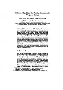
Maximal Cliques D

{ A, B, F } { B, C, E, F } : Maximum Clique {C, D, E }

F

E

Fig. 1. Example graph maximum clique. The number of vertices of a maximum clique in an induced subgraph G ( R) is denoted by ω ( R). Consider an example graph G0 = (V0 , E0 ) in Fig. 1, where V0 = { A, B, C, D, E, F } and E0 = {( A, B ), ( A, F ), ( B, C ), ( B, E ), ( B, F ), (C, D ), (C, E ), (C, F ), ( D, E ), ( E, F )}. All maximal cliques are { A, B, F }, { B, C, E, F } and {C, D, E }, where { B, C, E, F } is a maximum clique of size 4. Note that { B, C, E } is a clique, but is not a maximal clique since it is contained in a larger clique { B, C, E, F }.

3. Efficient algorithms for finding a maximum clique 3.1 A basic algorithm

One standard approach for finding a maximum clique is based on the branch-and-bound depth-first search method. Our algorithm begins with a small clique, and continues finding larger and larger cliques until one is found that can be verified to have the maximum size. More precisely, we maintain global variables Q, Qmax , where Q consists of vertices of a current clique, Qmax consists of vertices of the largest clique found so far. Let R ⊆ V consist of candidate vertices which may be added to Q. We begin the algorithm by letting Q : = ∅, Qmax : = ∅, and R : = V (the set of all vertices). We select a certain vertex p from R and add p to Q (Q : = Q ∪ { p}). Then we compute R p : = R ∩ Γ ( p) as the new set of candidate vertices. This procedure (EXPAND()) is applied recursively while R p = ∅ . Note here that if | Q| + | R| ≤ | Qmax | then Q ∪ R can contain only a clique that is smaller than or equal to | Qmax |, hence searching for R can be pruned in this case. This is a basic bounding condition. When R p = ∅ is reached, Q constitutes a maximal clique. If Q is maximal and | Q| > | Qmax | holds, Qmax is replaced by Q. We then backtrack by removing p from Q and R. We select a new vertex p from the resulting R and continue the same procedure until R = ∅. This is a well known basic algorithm for finding a maximum clique (see, e.g., (12; 10)) and is shown in detail in Fig. 2 as Algorithm BasicMC. The process can be represented by a search

www.intechopen.com

Efficient Algorithms for Finding Maximum and Efficient Algorithms for Finding Maximum and Maximal Cliques: Effective Tools for Bioinformatics Maximal Cliques: Effective Tools for Bioinformatics

627 3

procedure BasicMC (G = (V, E )) begin global Q : = ∅; global Qmax : = ∅; EXPAND(V); output Qmax end {of BasicMC} procedure EXPAND(R) begin while R = ∅ do p : = a vertex in R; if | Q| + | R| > | Qmax | then Q : = Q ∪ { p }; R p : = R ∩ Γ ( p ); if R p = ∅ then EXPAND(R p ) else (i.e., R p = ∅) if | Q| > | Qmax | then Qmax : = Q fi fi Q : = Q − { p} else return fi R : = R − { p} od end {of EXPAND} Fig. 2. Algorithm BasicMC forest that is similar to Fig. 3 (b). 3.2 Algorithm MCQ

We present a very simple and efficient algorithm MCQ (46) that is a direct extension of the previous BasicMC. 3.2.1 Pruning

One of the most important points to improve the efficiency of BasicMC is to strengthen the bounding condition in order to prune unnecessary searching. For a set R of vertices, let χ( R) be the chromatic number of R, i.e., the minimum number of colors so that all pairs of adjacent vertices are colored by different colors, and χ′ ( R) be an approximate chromatic number of R, i.e., a number of colors so that all pairs of adjacent vertices are colored by different colors. Then we have that ω ( R ) ≤ χ ( R ) ≤ χ ′ ( R ) ≤ | R |.

While obtaining χ( R) is also NP-hard, an appropriate χ′ ( R) could be a better upper bound of ω ( R) than | R|, and might be obtained with low overhead. Here, we employ very simple greedy or sequential approximate coloring to the vertices of R, as introduced in (42; 12; 43). Let positive integral numbers 1, 2, 3, ... stand for colors red, green, yellow, ... Coloring is

www.intechopen.com

4 628

Biomedical Engineering, Trends, Researches and Technologies Biomedical Engineering Trends in Electronics, Communications and Software

also called Numbering. For each p ∈ R, sequentially from the first vertex to the last, we assign a positive integral Number No [ p] which is as small as possible. That is, when the vertices in R = { p1 , p2 , . . . , pm } are arranged in this order, first let No [ p1 ] = 1, and subsequently, let No [ p2 ] = 2 if p2 ∈ Γ ( p1 ) else No [ p1 ] = 1, . . ., and so on. After Numbers are assigned to all vertices in R, we sort these vertices in ascending order with respect to their Numbers. We select p as the last (rightmost) vertex in R (at the 4th line in procedure EXPAND(R) in Fig. 2), then No [ p] = Max{ No [ q ] | q ∈ R}, that is an approximate chromatic number of R. So, we replace the basic bounding condition: if | Q| + | R| > | Qmax | then in Fig. 2 BasicMC, by the following new bounding condition: if | Q| + No [ p] > | Qmax | then. Numbering is applied every time prior to application of EXPAND(). Since the greedy Numbering to R is carried out in O(| R|2 )-time and is not so time-consuming, the new bounding condition can be very effective to reduce the search space with low overhead. 3.2.2 Initial sorting and simple numbering

We have shown in (12) that both search space and overall running time are reduced when one sorts the vertices in an ascending order with respect to their degrees prior to the application of a branch-and-bound depth-first search algorithm for finding a maximum clique. Carraghan and Pardalos (10) also employ a similar technique successfully. Therefore, at the beginning of our algorithm, we sort vertices in V in a descending order with respect to their degrees. This means that a vertex with the minimum degree is selected at the beginning of the while loop in EXPAND() in Fig. 2 since the selection of p is from the last (rightmost) to the first (leftmost). Furthermore, we initially assign Numbers to the vertices in V simply, so that No [V [i ]] = i for i ≤ Δ( G ), where Δ( G ) is the maximum degree of G, and No [V [i ]] = Δ( G ) + 1 for Δ( G ) + 1 ≤ i ≤ |V |. This initial Number has the desired property that No [ p] ≥ ω (V ) for any p in V while V = ∅. Thus, this simple initial Number suffices. This completes our explanation of the algorithm MCQ. See (46) for further details. 3.3 Algorithm MCR

Algorithm MCR (48) is an improved version of MCQ, where improvements are mainly for the initial sorting of the vertices. First, we alter the order of the vertices in V = {V [1], V [2], . . . , V [ n ]} so that in a subgraph of G = (V, E ) induced by a set of vertices V ′ = {V [1], V [2], . . . , V [i ]}, it holds that V [i ] always has the minimum degree in {V [1], V [2], . . . , V [i ]} for 1 ≤ i ≤ |V |. While the resulting order is identical to that of (10), it should be noted that time-consuming computation of the degree of vertices is carried out only at the beginning of MCR as in MCQ, and hence the overhead of the overall selection of vertices is very small, too. Here, the degrees of adjacent vertices are also taken into consideration. Numbering of the vertices is carried out in a similar way to MCQ, but more closely. The above considerations lead to an improved clique finding algorithm MCR. Example run We show an example run of MCR to an input graph G1 given in Fig. 3 (a). In the initial sorting, vertex G with the minimum degree is selected at first. Then, vertices F and E follow after G. Now the remaining vertices A, B, C, D are of the same minimum degree,

www.intechopen.com

Efficient Algorithms for Finding Maximum and Efficient Algorithms for Finding Maximum and Maximal Cliques: Effective Tools for Bioinformatics Maximal Cliques: Effective Tools for Bioinformatics

E

F

G

629 5

C

D

A

B

(a) An input graph G1 searching

No:

A,

B,

C,

D,

E,

F,

1,

2,

3,

4, √

5,

6,

Qmax = { A, B, C, D } No:

G 6

B, E, D

C, D, E

A, E, F

1, 2, 3 √

1, 2, 3 √

1, 1, 2 √

(b) A search forest of G1 Fig. 3. Example run of MCR and then Numbering is applied to this set of vertices to have No [ A] = 1, No [ B ] = 2, No [ C ] = 3, No [ D ] = 4. The other vertices are numbered as No [ E ] = 4 + 1 = 5, No [ F ] = 6 (= Δ ( G1 ) + 1), No [ G ] = 6. In addition, we have that Qmax = { A, B, C, D } (of size 4), since every degree of the vertices in the induced subgraph G1 ({ A, B, C, D }) is 3 = 4 − 1. The result of the initial sorting of vertices is shown at the top of Fig. 3 (b) and the corresponding numbers are just below these vertices. Subsequently, in EXPAND( ), the rightmost vertex G is selected to have Q = { G }, R G = Γ ( G ) = { A, E, F }. These vertices A, E, F are numbered 1, 1, 2 as shown in the second row of Fig. 3 (b).

www.intechopen.com

6 630

Biomedical Engineering, Trends, Researches and Technologies Biomedical Engineering Trends in Electronics, Communications and Software

√ Here, | Q| + No [ F ] = |{ G }| + 2 = 3 < | Qmax | = 4, then prune ( : checkmark in Fig. 3 (b)). The searching proceeds from the right to the left as shown in Fig. 3 (b). As a result, the maximum clique in G1 is Qmax = { A, B, C, D }. 3.4 Algorithm MCS

Algorithm MCS (39; 49; 50) is a further improved version of MCR. 3.4.1 New approximate coloring

When vertex r is selected, if No [r ] ≤ | Qmax | − | Q| then it is not necessary to search from vertex r by the bounding condition, as mentioned in Sect. 3.2.1. The number of vertices to be searched can be reduced if the Number No [ p] of vertex p for which No [ p] > | Qmax | − | Q| can be changed to a value less than or equal to | Qmax | − | Q|. When we encounter such vertex p with No [ p] > de f

| Qmax | − | Q| ( = Noth ) (Noth stands for Nothreshold), we attempt to change its Number in the following manner (16). Let No p denote the original value of No [ p]. [Re-NUMBER p] 1) Attempt to find a vertex q in Γ ( p) such that No [ q ] = k1 ≤ Noth , with | Ck1 | = 1. 2) If such q is found, then attempt to find Number k2 such that no vertex in Γ (q ) has Number k2 . 3) If such number k2 is found, then change the Numbers of q and p so that No [ q ] = k2 and No [ p] = k1 . (If no vertex q with Number k2 is found, nothing is done.) When the vertex q with Number k2 is found, No [ p] is changed from No p to k1 (≤ Noth ); thus, it is no longer necessary to search from p. 3.4.2 Adjunct ordered set of vertices for approximate coloring

The ordering of vertices plays an important role in the algorithm as demonstrated in (12; 10; 46; 48). In particular, the procedure Numbering strongly depends on the order of vertices, since it is a sequential coloring. In our new algorithm, we sort the vertices in the same way as in MCR (48) at the first stage. However, the vertices are disordered in the succeeding stages owing to the application of Re-NUMBER. In order to avoid this difficulty, we employ another adjunct ordered set Va of vertices for approximate coloring that preserves the order of vertices appropriately sorted in the first stage. Such a technique was first introduced in (38). We apply Numbering to vertices from the first (leftmost) to the last (rightmost) in the order maintained in Va , while we select a vertex in the ordered set R for searching, beginning from the last (rightmost) vertex and continuing up to the first (leftmost) vertex. An improved MCR obtained by introducing only the technique (38) in this section is named MCR*. 3.4.3 Reconstruction of the adjacency matrix

Each graph is stored as an adjacency matrix in the computer memory. Sequential Numbering is carried out according to the initial order of vertices in the adjunct ordered set Va , as described in Sect. 3.4.2. Taking this into account, we rename the vertices of the graph and reconstruct the adjacency matrix so that the vertices are consecutively ordered in a manner identical to the initial order of vertices obtained at the beginning of MCR. The above-mentioned reconstruction of the adjacency matrix (41) results in a more effective use of the cache memory. The new algorithm obtained by introducing all the techniques described in Sects. 3.4.1–3.4.3 in MCR is named MCS. Table 1 shows the running time required to solve some DIMACS

www.intechopen.com

Efficient Algorithms for Finding Maximum and Efficient Algorithms for Finding Maximum and Maximal Cliques: Effective Tools for Bioinformatics Maximal Cliques: Effective Tools for Bioinformatics

Graph brock400 1 block800 1 MANN a27 MANN a45 p hat500-2 p hat1000-2 san200 0.9 3 san400 0.7 2 san400 0.9 1 gen200 p0.9 44 gen400 p0.9 55 gen400 p0.9 65 C250.9

dfmax (18) 22,051 > 105 > 105 > 105 133 > 105 42,648 > 105 > 105 48,262

New (33)

> 2, 232 96

113

ILOG (35) 8,401 > 10, 667 14 > 10, 667 24 12,478 135 50 1,259

MCQ (46) 1,783 18,002 5.4 4,646 4.0 2,844 10 1.0 46.3

> 105

MCR (48) 1,771 17,789 2.5 3,090 3.1 2,434 0.16 0.3 3.4 5.39 5,846,951 > 2.5 × 107 44,214

631 7

MCS (50) 693 9,347 0.8 281 0.7 221 0.06 0.1 0.1 0.47 58,431 151,597 3,257

Table 1. Comparison of the running time [sec] benchmark graphs (18) by representative algorithms dfmax (18), New (33), ILOG (35), MCQ, MCR, and MCS, taken from (50). (105 seconds ≃ 1.16 days). Our user time ( T1 ) in (50) for DIMACS benchmark instances: r100.5, r200.5, r300.5, r400.5, and r500.5 are 1.57×10−3 , 4.15×10−2 , 0.359, 2.21, and 8.47 seconds, respectively. (Correction: These values described in the Appendix of (50) should be corrected as shown above. However, other values in (50) are computed based on the above correct values, hence other changes in (50) are not necessary.) While MCR* obtained by introducing the adjunct set Va of vertices for approximate coloring in Sect. 3.4.2 is almost always more efficient than MCR (38), combination of all the techniques in Sects. 3.4.1–3.4.3 makes it much more efficient to have MCS. The aim of the present study is to develop a faster algorithm whose use is not confined to any particular type of graphs. We can reduce the search space by sorting vertices in R in descending order with respect to their degrees before every application of approximate coloring, and hence reduce the overall running time for dense graphs (36; 21), but with the increase of the overall running time for nondense graphs. Appropriately controlled application of repeated sorting of vertices can make the algorithm more efficient for wider classes of graphs (21). Parallel processing for maximum-clique-finding is very promising in practice (41; 53). For practical applications, weighted graphs becomes more important. Algorithms for finding maximum-weighted cliques have also been developed. For example, see (45; 32; 30) for vertex-weighted graphs and (40) for edge-weighed graphs.

4. Efficient algorithm for generating all maximal cliques In addition to finding only one maximum clique, generating all maximal cliques is also important and has many diverse applications. In this section, we present a depth-first search algorithm CLIQUES (44; 47) for generating all maximal cliques of an undirected graph G = (V, E ), in which pruning methods are employed as in Bron and Kerbosch’s algorithm (7). All maximal cliques generated are output in a tree-like form.

www.intechopen.com

8 632

Biomedical Engineering, Trends, Researches and Technologies Biomedical Engineering Trends in Electronics, Communications and Software

4.1 Algorithm CLIQUES

The basic framework of CLIQUES is almost the same as BasicMC without the basic bounding condition. Here, we describe two methods to prune unnecessary parts of the search forest, which happened to be the same as in the Bron-Kerbosch algorithm (7). We regard the set SUBG (= V at the beginning) as an ordered set of vertices, and we continue to generate maximal cliques from vertices in SUBG step by step in this order First, let FI N I be a subset of vertices of SUBG that have been already processed by the algorithm. (FI N I is short for “finished”.) Then we denote by CAND the set of remaining candidates for expansion: CAND = SUBG − FI N I. So, we have SUBG = FI N I ∪ CAND

( FI N I ∩ CAND = ∅),

where FI N I = ∅ at the beginning. Consider the subgraph G (SUBGq ) with SUBGq = SUBG ∩ Γ (q ), and let SUBGq = FI N Iq ∪ CANDq (FI N Iq ∩ CANDq = ∅),

where FI N Iq = FI N I ∩ Γ (q ) and CANDq = CAND ∩ Γ (q ). Then only the vertices in CANDq can be candidates for expanding the complete subgraph Q ∪ {q } to find new larger cliques. Secondly, given a certain vertex u ∈ SUBG, suppose that all the maximal cliques containing Q ∪ {u } have been generated. Then every new maximal clique containing Q, but not Q ∪ {u }, must contain at least one vertex q ∈ SUBG − Γ (u ). Taking the previously described pruning method also into consideration, the only search subtrees to be expanded are from vertices in (SUBG − SUBG ∩ Γ (u )) − FI N I = CAND − Γ (u ). Here, in order to minimize | CAND − Γ (u ) |, we choose such vertex u ∈ SUBG to be the one which maximizes | CAND ∩ Γ (u ) |. This is essential to establish the optimality of the worst-case time-complexity of CLIQUES. Our algorithm CLIQUES (47) for generating all maximal cliques is shown in Fig. 4. Here, if Q is a maximal clique that is found at statement 2, then the algorithm only prints out a string of characters “clique, instead of Q itself at statement 3. Otherwise, it is impossible to achieve the worst-case running time of O(3n/3 ) for an n -vertex graph. Instead, in addition to printing “clique” at statement 3, we print out q followed by a comma at statement 7 every time q is picked out as a new element of a larger clique, and we print out a string of characters “back,” at statement 12 after q is moved from CAND to FI N I at statement 11. We can easily obtain a tree representation of all the maximal cliques from the sequence printed by statements 3, 7, and 12. The output in a tree-like format is also important practically, since it saves space in the output file. 4.2 Time-complexity of CLIQUES

We have proved that the worst-case time-complexity is O(3n/3 ) for an n-vertex graph (47). This is optimal as a function of n, since there exist up to 3n/3 cliques in an n-vertex graph (29). The algorithm is also demonstrated to run fast in practice by computational experiments. Table 2 shows the running time required to solve some DIMACS benchmark graphs by representative algorithms CLIQUE (11), AMC (24), AMC* (24), and CLIQUES, taken from (47). For practical applications, enumeration of pseudo cliques sometimes becomes more important (52).

www.intechopen.com

Efficient Algorithms for Finding Maximum and Efficient Algorithms for Finding Maximum and Maximal Cliques: Effective Tools for Bioinformatics Maximal Cliques: Effective Tools for Bioinformatics

633 9

procedure CLIQUES(G) begin 1 : EXPAND(V,V) end of CLIQUES

2: 3: 4: 5: 6: 7: 8: 9: 10 : 11 : 12 :

procedure EXPAND(SUBG, CAND) begin if SUBG = ∅ then print (“clique,”) else u : = a vertex u in SUBG which maximizes | CAND ∩ Γ (u ) |; while CAND − Γ (u ) = ∅ do q : = a vertex in (CAND − Γ (u )); print (q, “,”); SUBGq : = SUBG ∩ Γ (q ); CANDq : = CAND ∩ Γ (q ); EXPAND(SUBGq , CANDq ); CAND : = CAND − {q }; print (“back,”) od fi end of EXPAND

Fig. 4. Algorithm CLIQUES Graph brock200 2 johnson16-2-4 keller4 p hat300-2

CLIQUE (11) 181.4 908 3,447 > 86, 400

AMC (24) 75.2 151 1,146 16,036

AMC* (24) 35.9 153 491 4,130

CLIQUES (47) 0.7 4 5 100

Table 2. Comparison of the running time [sec]

5. Applications to bioinformatics 5.1 Analysis of protein structures

In this subsection, we show applications of maximum clique algorithms to the following three problems on protein structure analysis: (i) protein structure alignment, (ii) protein side-chain packing, (iii) protein threading. Since there are many references on these problems, we only cite references that present the methods shown here. Most of other relevant references can be reached from those references. Furthermore, we present here only the definitions of the problems and reductions to clique problems. Readers interested in details such as results of computational experiments are referred to the original papers (1; 2; 3; 4; 8). 5.1.1 Protein structure alignment

Comparison of protein structures is very important for understanding the functions of proteins because proteins with similar structures often have common functions. Pairwise comparison of proteins is usually done via protein structure alignment using some scoring scheme, where an alignment is a mapping of amino acids between two proteins. Because of

www.intechopen.com

10 634

Biomedical Engineering, Trends, Researches and Technologies Biomedical Engineering Trends in Electronics, Communications and Software

P

p1

G(V,E)

p2 p3

Q

q3 q1

( p2 , q1 ) ( p3 , q1 )

( p1 , q1 )

q2 q4

( p1 , q2 )

( p3 , q2 )

( p1 , q3 )

( p3 , q3 )

( p1 , q4 )

( p3 , q4 )

Fig. 5. Reduction from protein structure alignment to maximum clique. Maximum clique shown by bold lines (right) corresponds to protein structure alignment shown by dotted lines (left). its importance, many methods have been proposed for protein structure alignment. However, most existing methods are heuristic ones in which optimality of the solution is not guaranteed. Bahadur et al. developed a clique-based method for computing structure alignment under some local similarity measure (2). Let P = (p1 , p2 , . . . , p m ) be a sequence of three-dimensional positions of amino acids (precisely, positions of Cα atoms) in a protein. Let Q = (q1 , q2 , . . . , q n ) be a sequence of positions of amino acids of another protein. For two points x and y, | x − y | denotes the Euclidean distance between x and y. Let f ( x ) be a function from the set of non-negative reals to the set of reals no less than 1.0. We call a sequence of pairs M = ((p i1 , q i1 ), . . . , (p il , q il )) an alignment under non-uniform distortion if the following conditions are satisfied: – ik < ih and jk < jh hold for all k < h,   | q jh − q jk | 1 – (∀k)(∀h = k) < < f (r ) , f (r ) | p jh − p jk | where r = min{| q jh − q jk |, | p jh − p jk |}. Then, protein structure alignment is defined as the problem of finding a longest alignment (i.e., l is the maximum). It is known that protein structure alignment is NP-hard under this definition. This protein structure alignment problem can be reduced to the maximum clique problem in a simple way (see Fig. 5). we construct an undirected graph G (V, E ) by V

=

{ (p i , q j ) | i = 1, . . . , m, j = 1, . . . , n },

E

=

{ {(p i , q j ), (p k , q h )} | i < k, j < h,

|qh − q j | 1 < < f (r ) } . f (r ) |pk − pi |

Then, it is straight-forward to see that a maximum clique corresponds to a longest alignment. 5.1.2 Protein side-chain packing

The protein side-chain packing problem is, given an amino acid sequence and spatial information on the main chain, to find side-chain conformation with the minimum potential energy. In most cases, it is defined as a problem of seeking a set of (χ1 , χ2 , . . .) angles whose potential energy becomes the minimum, where positions of atoms in the main chain are fixed. This problem is important for prediction of detailed structures of proteins because such prediction methods as protein threading cannot determine positions of atoms in the side-chains. It is known that protein side-chain packing is NP-hard and thus various heuristic methods have

www.intechopen.com

Efficient Algorithms for Finding Maximum and Efficient Algorithms for Finding Maximum and Maximal Cliques: Effective Tools for Bioinformatics Maximal Cliques: Effective Tools for Bioinformatics

635 11

been proposed. Here, we briefly review a clique-based approach to protein side-chain packing (2; 3; 8). Let R = {r1 , . . . , rn } be the set of amino acid residues in a protein. Here, we only consider χ1 angles and then assume that positions of atoms in a side-chain are rotated around the χ1 axis. Let ri,k be the ith residue whose side-chain atoms are rotated by (2πk)/K radian, where we can modify the problem and method so that the rotation angles can take other discrete values. We say that residue ri,k collides with the main chain if the minimum distance between the ˚ We say that residue atoms in ri,k and the atoms in the main chain is less than a threshold L1 A. ri,k collides with residue r j,h if the minimum distance between the atoms in ri,k and the atoms ˚ We define an undirected graph G (V; E ) by in r j,h is less than L2 A. V E

= =

{ ri,k | ri,k does not collide with the main chain }, { {ri,k , r j,h } | ri,k does not collide with r j,h }.

Then, it is straight-forward to see that a clique with size n corresponds to a consistent configuration of side chains (i.e., side-chain conformation with no collisions). We can extend this reduction so that potential energy can be taken into account by using the maximum edge-weighted clique problem. 5.1.3 Protein threading

Protein threading is one of the prediction methods for three-dimensional protein structures. The purpose of protein threading is to seek for a protein structure in a database which best matches a given protein sequence (whose structure is to be predicted) using some score function. In order to evaluate the extent of match, it is required to compute an optimal alignment between an amino acid sequence S = s1 s2 . . . sn and a known protein structure P = (p1 , p2 , . . . , p m ), where si and p j denote the ith amino acid and the jth residue position, respectively. As in protein structure alignment, a sequence of pairs ((si1 , p j1 ), (si2 , p j2 ), . . . , (sil , p jl )) is called an alignment (or, a threading) between S and P if ik < ih and jk < jh hold for all k < h. Let g(sik , sih , p jk , p jh ) give a score (e.g., pseudo energy) between residue positions of p jk and p jh when amino acids sik and sih are assigned to positions of p jk and p jh , respectively. Then, protein threading is defined as a problem of finding an optimal alignment that minimizes the pseudo energy:

∑ g ( s i , s i , p j , p j ), k

h

k

h

k