asperity surface contact model is presented that provides real-time rendering of ... implementation of the friction model in virtual environments are also discussed ...
Proceedings of EuroHaptics 2004, Munich Germany, June 5-7, 2004.
Efficient and Accurate Simulation of Friction using a Multi-asperity Surface Contact Model Yinghui Zhang, Roger Phillips Department of Computer Science, The University of Hull, Hull, HU6 7RX, UK {y.zhang, r.phillips}@hull.ac.uk
Abstract. This paper describes a new friction model, called the “brush model“, suitable for haptic rendering in virtual environments. A novel two-layer multiasperity surface contact model is presented that provides real-time rendering of friction forces at haptic refresh rates. This new friction model has several advantages; of particular importance is the accuracy with which it handles static friction and the transition to sliding motion. This paper focuses on one such feature of static friction, namely the undesirable motion drift artefact; results are presented which show that our model behaves correctly. Issues relating to implementation of the friction model in virtual environments are also discussed.
1 Introduction Our interaction with the physical world is through our sensations systems such as auditory, visual, tactile, etc. Haptic technologies can provide us with a sense of touch in virtual environments. Investigations have shown that the presence of force feedback can greatly enrich a person’s virtual experiences, and make the simulation more realistic; moreover, it can improve the performance of manipulative tasks by operators [1]. As friction is fundamental to our tactile interaction with the real world, friction modelling in haptics is deemed important. Without friction, objects in contact in a virtual environment often feel slippery and thus do not mimic reality sufficiently for many virtual environment applications. The simulation of friction for haptic rendering in virtual environments is challenging. Friction as a physical phenomenon is very complicated and the underlying mechanism is still not fully understood. Other issues associated with the simulation of a friction model for haptic interaction also arise; for example: some friction models cause the haptic simulation to become unstable due to the presence of noise in measuring velocity [2], and the requirement of some models to detect zero velocity may cause incorrect simulation results. Another significant constraint is being able simulate friction accurately whilst achieving a haptic refresh rate of 1 kHz for virtual environments. Several friction models had been proposed by researchers. Haessig and Friedland [3] described a bristle model, in which two kinds of bristles, namely, rigid bristles and pliable bristles, are used to simulate the interaction of asperities between the
36
contacting surfaces. However, this model is not suitable for real time simulation due to its expensive computational costs. Chen et al. [13] also presented a bristle model using only one bristle. Nahvi et al [10] proposed a modified Coulomb’s model. Its evaluation by Gosline [11] concluded that this model is also not suitable for haptic simulation. This paper describes a new friction model that simulates in a simplified manner the behaviour of asperities for contacting surfaces. We call this new model the “brush model”, since for the two contacting surfaces one is represented by a brush of flexible bristles whilst the other is represented by a smooth surface. The simplifications made in the simulation make it very computationally efficient whilst producing an accurate simulation of friction. The next section of this paper describes the proposed surface contact model and the mathematical derivation of our model for the simulation of friction. A full exposition of the behaviour and features of our model is provided elsewhere [9]. This paper focuses on one feature of behaviour of static friction, namely: to demonstrate that our model does not suffer from the spurious motion drift phenomenon [5] that occurs in many simpler models of friction. Section 4 then describes the virtual environment used for experimentation and qualitative assessment of friction. Section 5 discusses the extent and benefits of this model. The paper finishes with conclusions and the scope for future work.
2 A New Multi-asperity Friction Model --- Brush Model 2.1 A Two-layer Multi-asperity Surface Contact Model Our surface contact model features a novel two-layer architecture. In the geometric layer (the underlying layer) a brush-like behaviour of flexible bristles is employed to define how the contacting surfaces interact. Based on this, a mathematical equation is developed in the abstract layer (the second layer) describing the relationship of normal pressure and the number of bristles in contact. Geometric Layer. In our model of two contacting surfaces, the interaction between asperities is simplified by supposing one surface is stationary and smooth (see surface B in Fig. 1) with the other surface being covered with flexible bristles (see surface A in Fig. 1) which make contact with the smooth surface. The length of the bristles is governed by a probability distribution ϕ (h) , where h is the height of a bristle. These bristles are distributed randomly over the surface area of A in contact with surface B. According to the Coulomb’s law, the distribution of bristles does not have any significant effects on the resulting friction forces. Therefore, the model does not need to know the actual locations of bristles on surface A. When relative motion starts, bristles in contact will bend to generate tangential resistance which is calculated by Dahl’s spring model [6]. When the deflection of a bristle exceeds the maximum deflection displacement, the bristle snaps, and is then replaced by another bristle. The snap distance is randomly varied for the set of bristles. Physically this variation in snap distance is analogous to the variations between asperities on the actual surface. All bristles have uniform stiffness. The frictional
37
force of the contacting surfaces is calculated by summing together the effects of all the bristles of surface A that actually make contact with surface B.
Normal load
Surface A
Motion direction
h Surface B
(a)
d (b)
Fig. 1. (a) Bristles in still state; (b) Bristles bending.
Along the normal direction, the interacting bristles deform to carry the normal pressure. A linear spring model is used to calculate the normal load on each bristle. As the normal pressure varies so does the number of bristles in contact, which represents the true contact area. The Abstract Layer. To efficiently determine how many bristles are in contact under certain normal pressure, a mathematical method has been derived. Let ς denote the number of bristles in contact, N is the normal pressure. The relationship ς = ς (N ) has been build up, see section 2.3. In summary, the computationally efficiency of the brush model in simulating friction is achieved by the advantages of the two-layer architecture: 1) explicit collision detection between bristles and the opposite surface is not required; 2) the location of bristles is not required; 3) the model is not constrained by surface geometry; the contact surfaces can be flat or curved surfaces. This feature distinguishes our brush model from other multi-asperity based friction models such as the bristle model [3]. In [3], the surface contact model only comprised one layer; the two surfaces are all attached with bristles. Therefore, the location of bristles and the collision detection between them are essential for obtaining the overall tangential forces. Moreover, allocating bristles along a curved surface can be very inefficient. 2.2 Calculation of Friction Forces Let z λ denote the deflection of bristle λ . The motion of a bristle is modelled as: dz λ dx (1) = , 0 ≤ zλ ≤ δ λ dt dt where x is the relative displacement of the sliding surface, δ λ is the maximum deflection displacement of bristle λ . Equation (1) indicates that a bristle moves at the same speed as the sliding surface. When the deflection z λ exceeds δ λ , bristle λ snaps
and z λ will be reset to zero.
38
By using Dahl’s spring model, the local friction at each bristle is given by:
dz λ (2) dt where σ 0 is the stiffness of a bristle and σ 1 is the damper coefficient. The addition of a damper term is to prevent vibration so as to give a stable motion. By summing up the local friction (equation (2)) for all the bristles in contact between the two surfaces, the total friction for solid-to-solid contact is then obtained: dz (3) F= (σ 0 z λ + σ 1 λ ) 1≤ λ ≤ς dt where ς is the number of bristles in contact. To take account of viscous friction for lubricated surfaces, an additional term which is proportional to velocity needs to be added into equation (3) to give: dz dx (σ 0 z λ + σ 1 λ ) + σ 2 (4) F= 1≤ λ ≤ς dt dt where σ 2 is the viscous coefficient. As oscillation can occur in the sticking phase, f local = σ 0 z λ + σ 1
the damper coefficient σ 1 is chosen to be a function of velocity, which is always activated whenever the velocity is low. We choose σ 1 with a form similar to that of Canudas de et al. [7]:
σ 1 ( v λ ) = σ 1 e − vλ
vs
(5)
where σ 1 and v s are constants. v s is also known as the Stribeck velocity. 2.3 Deriving the Number of Bristles in Contact ς To derive the relationship between the normal load N and the number of bristles in contact ς , let’s suppose ϕ (h) (see section 2.2) is an exponential distribution function [8], i.e. 1 −h (6) ϕ (h) = e σ
σ
where σ is the standard deviation and h is the length of a bristle (see Fig. 1(a)). Using Hook’s law, the normal load on a bristle of height h can be calculated by σ ⊥ (h − d ) , where σ ⊥ is the unified normal stiffness of bristles, d is the separation between the contact surfaces (see Fig.1). The total normal pressure carried by bristles is then given by ∞
N = ∆η σ ⊥ (h − d )ϕ (h)dh = ∆ησ ⊥ σe
−d
σ
(7)
d where ∆ is the apparent contact area and η is the density of bristles. As the bristles in contact represent the true contact area, ς can be estimated by
∞
ς = ∆η ϕ (h) dh = ∆ηe d
39
−d
σ
(8)
Comparing equation (7) and (8), the relationship between N and ς is then estimated by:
ς = N σσ −6
(9)
⊥
where σ = 10 m is a suitable value for most of industrial surfaces [4].
3 Motion Drift Dupont et al. [5] reported that single-state friction models characteristically exhibit spurious positional drift of two surfaces in contact. For example, consider a small disturbance being applied to a block resting on a frictional slope. In the real world the block stays in equilibrium and maintains its position on the slope. However, singlestate friction models typically predict that this causes slow motion drift of the block down the slope. It is particularly undesirable when simulating friction in virtual environments as it contradicts the expectations and daily experiences of users. Simulation tests have been performed on our model to investigate this phenomenon. The results obtained show that our friction model does not drift (see Fig. 2). The profile of applied force chosen was similar to that of Dupont et al. [5]. Friction Force [N]
Applied Force [N]
0.25
0.2
0.15
0.1
0.05
0 0
0.5
1
1.5
2
2.5
3
3.5
0. 25 0.2 0. 15 0.1 0. 05 0 0
0.5
1.5
1
2
2.5
Pre-sliding Displacement [ 10 µm ]
Time [s] (a)
(b)
Fig. 2. Simulation test for investigating undesirable motion drift between unlubricated surfaces. (a) Profile of the applied force; (b) Effect of friction on the applied force in terms of pre-sliding displacement. The circle of movement around 20 m clearly shows that the drift does not occur.
Besides motion drift, various simulations test have been performed to investigate the dynamic behaviour of our friction model. These tests include stick-slip motion, friction lag, Stribeck effect, pre-sliding displacement, variation of breakaway forces, etc. The simulation results have shown that our friction model captures accurately most friction phenomena observed experimentally and these are reported in [9]. All these simulation tests were performed in MathCAD.
40
4 Haptic Rendering of Friction in Virtual Environments 4.1 Development Environment and Software Architecture
Various simulations of the new friction model within a virtual environment have been performed using a PHANToM 1.0 force feedback device to provide contact forces. The simulations were ran on a PC system with a PIII 1GHz Intel processor and an Nvidia Geforce 2 graphics card. The software was developed using Visual C++ 6.0 and GHOST SDK 3.0. A simple virtual environment has been created to investigate the efficiency and to qualitatively assess the behaviour of our model of friction. This virtual environment comprises of 3 side walls, a roof and a floor with a block placed on the floor. Users can apply forces to the block and feel the effects of friction via a PHANToM 1.0 haptic device. Via a GUI, users can adjust parameters of the friction model to control bristle length, bristle stiffness, coefficients for damping and lubrication, etc. The graphic and haptic displays of the scene graph are rendered by two simulation loops, namely: 1) the haptic simulation loop and 2) the graphic simulation loop (see Fig. 3). All collision detections and computations of contact forces are conducted in the haptic simulation loop. Communications between the two loops occurs with the graphic loop obtaining the position of the block from the haptic loop prior to rendering the scene. To meet the haptic refresh rate of 1 kHz, the number of bristles in simulations was limited to 900. Keyboard/Mouse Input Haptic Interface Input
GUI
Haptic Loop 1. Calculate new position and velocity. 2. Collision detection. 3. Calculate friction forces. 4. Generate hatpic feedback.
Graphic Loop 1. Inquire position from haptic loop 2. Display scene at new position
Fig. 3. Two-loop software architecture.
This simple virtual environment demonstrated qualitatively the realistic feel of friction between contact surfaces. Numerous validation experiments are planned to quantitatively assess the improvements. The pseudo-code of the implementation of our friction model is listed below. Input: Vector velocity, float deltaT; Output: Vector friction Vector x = velocity * deltaT;
41
for ( i =0; i