Jul 20, 2008 - example of a multiagent plan coordination problem, motivating how such .... discuss approximation methods for coordinating agent tasks with different ...... queue is a Last In, First Out (LIFO) queue, meaning that states are ...
Efficient and Distributable Methods for Solving the Multiagent Plan Coordination Problem Jeffrey Cox and Edmund Durfee Department of Electrical Engineering and Computer Science University of Michigan Ann Arbor, MI 48109 {jeffcox, durfee}@umich.edu July 20, 2008
Abstract Coordination can be required whenever multiple agents plan to achieve their individual goals independently, but might mutually benefit by coordinating their plans to avoid working at cross purposes or duplicating effort. Although variations of such problems have been studied in the literature, there is as yet no agreement over a general characterization of them. In this paper, we formally define a common coordination problem subclass, which we call the Multiagent Plan Coordination Problem, that is rich enough to represent a wide variety of multiagent coordination problems. We then describe a general framework that extends the partial-order, causal-link plan representation to the multiagent case, and that treats coordination as a form of iterative repair of plan flaws between agents. We show that this algorithmic formulation can scale to the multiagent case better than can a straightforward application of the existing plan coordination techniques, highlighting fundamental differences between our algorithmic framework and these earlier approaches. We then examine whether and how the Multiagent Plan Coordination Problem can be cast as a Distributed Constraint Optimization Problem (DCOP). We do so using ADOPT, a state-of-the-art system that can solve DCOPs in an asynchronous, parallel manner us-
1
ing local communication between individual computational agents. We conclude with a discussion of possible extensions of our work.
2
1
Introduction
Agents that share an environment and that want to achieve collective (as opposed to selfish) goals need to coordinate their planned actions at least to avoid interfering with each other, and preferably to help each other. This paper is about a framework for solving an important class of coordination problems efficiently that supports the distribution of coordination problem solving efforts across the involved agents. We call the particular class of coordination problems we solve the Multiagent Plan Coordination Problem (MPCP), where the problem input is a set of individual agents’ plans (typically one per agent), each directed toward achieving a distinct (sub)goal of interest to the particular agent. The solution output for a MPCP is a set of modified plans, where each input plan has been modified (if necessary) by the addition of constraints (to prevent unintended interference) and by removing actions (to reduce collective effort) given the plans of the other agents. We believe the MPCP is a useful label to describe the class of problems we consider. This is not to suggest that our definition of the Multiagent Plan Coordination Problem will encompass all possible variations of multiagent plan coordination, but we do believe that our definition of the Multiagent Plan Coordination Problem is rich enough to represent a wide variety of problems. In fact, the MPCP arises in many multiagent application domains. One example of particular interest in our work is in coordinating the activities of partners in a military coalition (to avoid catastrophic interference like “friendly fire” and duplicated effort like in securing roadways and airports). However, the issue of coordinating activities between actors who are pursuing their own objectives in a shared environment (e.g. subcontractors working on a building, airlines operating in an alliance, etc.) occurs widely. Our work develops a general framework for solving the MPCP that can be applied in any of these kinds of domains. Plan coordination works best when agents’ plans are loosely-coupled, meaning that their individual plans for the most part do not contain actions that interact with each other. Otherwise, the agents might benefit more from centralized planning. This characteristic of the plan coordination problem has lead to solution techniques that emphasize viewing the coordination process as effectively merging the individually-formed plans into a coordinated whole. Plan merging techniques have been developed both in the context of single agents (where plans for different subgoals are generated separately and then merged into an overall plan for an agent),
3
and for multiple agents. The emphasis in most of the prior work has been on analyzing the ways that possible events could play out over time given the separate plans, and identifying problematic (sets of) states that could arise, requiring adjustments to the separate plans to avoid these states. In contrast to prior efforts, we motivate and develop an alternative strategy for MPCPs that works by repairing coordination flaws directly in the multiagent plan space, rather than by projecting the effects of the agents’ concurrent plans into the agents’ joint state space and then working backward from all the problematic states into adjustments to the plans to preclude them. Our analyses indicate that our new approach is more efficient at exploiting the looselycoupled nature of MPCPs. Building on this result, we describe our investigations into the question of whether the parallel computational resources of the agents being coordinated can be exploited by extending the MPCP formulation we have developed into a distributed constraint optimization problem (DCOP), and we describe how this distributed formulation can be solved using an off-the-shelf DCOP solver. The remainder of this paper is structured as follows. In section 2, we give a brief, illustrative example of a multiagent plan coordination problem, motivating how such problems can arise and the kinds of repairs that can fix coordination flaws between plans. In Section 3, we examine prior work on the problem of coordination and discuss the limitations of that work when it comes to solving the kinds of problems of interest in this paper. In Section 4, we describe our formalization of the Multiagent Plan Coordination Problem (MPCP), characterize our planspace search algorithm designed to solve the MPCP, and evaluate its performance. In Section 5, we show how the MPCP can be cast as a Distributed Constraint Optimization Problem (DCOP). After characterizing the DCOP formulation of the MPCP, we then illustrate how we can take it and (with some appropriate modifications) use ADOPT, a DCOP solver, to solve the MPCP. Finally, in Section 6 we present our conclusions and future work. Preliminary versions of this work have previously appeared elsewhere [7] [8]. This paper extends and improves on these publications by: • Providing better characterizations of the concepts of multiagent plan interaction, in Section 2.
4
• Changing the definition of plan flaws in the Multiagent Plan Coordination Problem to create a richer problem representation, in Section 4.4. Specifically, rather than characterizing positive interactions between agents as plan step merge flaws, it creates a more general definition of redundancy. • Defining a completely new algorithm to solve the MPCP (based on a causal-link adjustment method) that is complete given the expanded problem definition of the MPCP, in Section 4.5. • Presenting additional empirical results to demonstrate the effectiveness of our algorithm, comparing it against Mali’s work on Planning as Satisfiability, in Section 4.7. • Updating the DCOP encoding of the MPCP to account for its richer representation, in Section 5.
2
Motivating Example
To illustrate the more general problem of multiagent plan coordination, consider a set of agent convoys, each with a separate plan to move along routes through a common environment to reach its goals. In Figure 1 there are two agent convoys: a tank convoy and a truck convoy. Although each convoy has its own goals and thus will operate separately, there exist possible interactions between their plans. At various points along their routes, overgrown roadways may need to be cleared before the agents can proceed. If one agent is to clear the roadway, the other can make use of the cleared path without expending its own effort. Similarly, portable bridges may need to be constructed to traverse more difficult terrain, such as swamps and small rivers. Agents may share in the deployment of these bridges for mutual benefit, thus avoiding redundant effort. Both of these two kinds of interactions can be considered positive interactions, as both agents do not need to clear the road, and if they synchronize correctly one convoy can make use of the other’s temporary bridge (though not simultaneously). The difference between the two types is their temporal extent, as once the road is cleared, it will stay cleared (for at least as long as the agents need to use it), whereas the portable bridge will only be available while the agent that puts it down is still using it. 5
Single-User Bridge (Temporary Negative) Bridge Point (Temporary Positive)
Truck Goal
Dirt Road (Permanent Negative)
Overgrown Road (Permanent Positive)
Tank Goal
A A
Figure 1: Convoy Example Other possible agent interactions may not be so mutually beneficial. For example, parts of the routes the convoys traverse may only permit a single convoy to pass at a time (such as a bridge, temporary or permanent, that cannot support more than one convoy simultaneously), and other roads may be rendered impassable to other agents once an agent crosses it (for example, the tank convoy may tear up dirt roads, rendering them impassable by vehicles without treads). Both of these two kinds of interactions can be considered negative interactions between the plans of different agents. Like in the case of the positive interactions, the difference between the types is their temporal extent, either temporary (use of a bridge) or permanent (destruction of a roadbed). The corresponding plans of the agents, with dotted lines enumerating their plan interactions, are given in Figure 2. Clearly, in order for the two convoys to carry out their plans, they should resolve their plan interactions both to improve their execution efficiency and to prevent plan failure. The first interaction is contention over the single-user bridge. The second involves the redundant Deploy Mobile Bridge steps, as only one convoy needs to set up a mobile bridge. The third depends on how the second is dealt with, as the agents only contend for the single-user mobile bridge if they share it. The fourth also depends on how the second is dealt with, as, if the agents share the same bridge, then the bridge cannot be removed until both agents have crossed it. The fifth involves the Traverse Dirt Road actions, as once the tank convoy uses the road, the truck convoy cannot. Finally, the sixth involves the redundant Clear Block actions, 6
Tank Plan Initial State
Cross Bridge
Move To River
Deploy Mobile Bridge
Cross Bridge
2
3
1
Remove Mobile Bridge
Move To Block
Traverse Dirt Road
Clear Block
5
4
Goal
6
Truck Plan Initial State
Cross Bridge
Remove Mobile Bridge
Deploy Mobile Bridge
Move To River
Move To Block
Traverse Dirt Road
Cross Bridge
Clear Block
Goal
Figure 2: Convoy Plans with Identified Interactions Tank Plan Initial State
Cross Bridge
Move To River
Cross Bridge
Move To Block
Traverse Dirt Road
Clear Block
Goal
Truck Plan Initial State
Cross Bridge
Remove Mobile Bridge
Deploy Mobile Bridge
Move To River
Traverse Dirt Road
Move To Block
Cross Bridge
Goal
Figure 3: Coordinated Convoy Plans which clear the roadblocks. Figure 3 illustrates the plans of the agents after they have been coordinated by resolving the described interactions. The first bridge conflict is avoided by temporally ordering the tank convoy’s bridge crossing actions before the bridge crossing actions of the truck convoy. Second,
7
the redundant Deploy Mobile Bridge (and accompanying Remove Mobile Bridge) steps of the tank convoy have been removed, as only one convoy needs to set up a mobile bridge. To ensure that both convoys cross the bridge before it is removed, both Cross Bridge actions are ordered before the Remove Mobile Bridge action, and the Cross Bridge actions of the two convoys are serialized to prevent over-utilization of the mobile bridge. To prevent the tank convoy from destroying the road before the truck convoy can pass, the tank convoy’s Traverse Dirt Road step is ordered after the truck convoy’s step. Finally, the Clear Block action of the truck convoy has been removed, as the truck convoy can rely on the tank convoy to clear the obstruction. The coordinated plan is consistent, in that all negative interactions have been resolved, and optimal, based on a simple optimality definition of minimizing the aggregate cost of the steps in the coordinated plan (assuming each step has a cost of one), as no other set of steps will allow the agents to achieve their goals any more efficiently.
3
Related Work
In this section, we provide a brief overview of previous work on the problem of multiagent plan coordination. Because our focus is on the problem of coordinating agent plans, we limit the scope of this section to include work on coordination, and not the more general (and more difficult) problem of multiagent planning, as surveyed in [10] and [9].
3.1
Multiagent Coordination
Multiple agents operating in a shared environment might, either by necessity or by choice, want to identify and then either avoid or exploit potential interactions between their activities. Such interactions can arise in a variety of circumstances, including when there exist scarce resources that the agents must share, or when one agent operates on the same part of the world that another agent does. There has been a great deal of research on possible approaches to solving these problems, including work with Contract Nets [29], market-based multiagent resource allocation methods [35], as well as the development of social laws that facilitate cooperation between agents [15].
8
However, much of this work assumes that information about the points of interaction (e.g., resources) are predefined and thus known to the coordination method at the outset of the problem. In contrast, our work makes no such assumptions, and thus requires the coordination framework we use to first identify possible interactions between the plans of agents, and then explore possible ways of responding to the interactions.
3.2
Multiagent Plan Coordination
Multiagent plan coordination has been an issue of interest in the multiagent systems community for many years, dating at least back to the seminal work of Georgeff [14]. Georgeff’s multiagent planning work concentrated on the problem of resolving conflicts and potential clobbering actions between the plans of different agents with different goals to ensure safe plan execution. Thus, it emphasized finding consistency flaws, and resolving them by inserting synchronizing communication actions. Georgeff modeled individual plan actions as consisting of a series of states, represented as an unordered set of conditions, where these conditions were considered to hold during the action. This specification of “during conditions” allows his system to reason about the implications of actions occurring in parallel. Specifically, actions with conflicting “during conditions” could not be executed simultaneously. In the majority of work since, the emphasis of coordination has been on ensuring consistency: that the actions of the various agents are selected or ordered (synchronized) so as to avoid agents interfering with each other. Because negative interactions could entirely prevent goals from being achieved, it is important to predict and avoid them. Research has also been done on multiagent plan coordination to exploit potential positive interactions. The work by von Martial on so-called “favor” relations [33] brought these issues to the fore. In general, failure to identify and exploit such interactions is not as catastrophic as failure to predict and resolve negative interactions, and so somewhat less attention has been paid to this problem over the years. Ephrati and Rosenschein [12] developed a method for coordinating the plans of multiple agents, where the plans were formed separately in response to subgoals that were assigned to the agents. Their method is general in the sense that it can resolve negative interactions but also exploit positive interactions. However, as we have shown elsewhere [6], Ephrati’s
9
algorithm does not scale well as the number of agent plans to be coordinated increases, even if the plans are loosely coupled, and thus falls short of fully addressing the coordination problem we consider here. Tonino et al. [32] have described algorithms for coordinating the plans of multiple agents based on an underutilization of free resources. In their approach, once a free resource (i.e., an effect or postcondition) of a plan step has been used to replace an output resource of another plan step, it is no longer available to replace the output resources of other plan steps. Thus, their system considers a different problem (more like a supply chain) than the one we consider, where in our case a single step can produce a state-changing effect that can satisfy the preconditions of many other steps of other agents. Much of the more recent work on multi-agent planning and plan coordination has emphasized MDP-based formulations, such as DEC-MDPs. These include algorithms for coordinating (or merging) individual agent policies into a joint policy. For example, the JESP approach of Nair et al. [25] has agents iteratively modify their policies in best-response to the policies of other agents until they converge (no agent needs to adjust its policy further). Centralized approaches for problems with limited coupling (e.g., transition or reward independence), include Becker’s coverage set algorithm [3], as well as the bilinear programming techniques of Petrik and Zilberstein [27]. Rather than discovering and resolving coordination flaws based on existing agent plans, these approaches often assume that the effects that one agent can have on another are pre-defined, such that agents can explicitly negotiate over their interactions prior to, or concurrently with, formulating their local plans [2, 22, 36]. The recent work that is closest to ours is that of Steenhuisen and Witteveen [30, 31], who discuss approximation methods for coordinating agent tasks with different degrees of plan coupling. However, their definition of plan coupling is fundamentally different from our own. Specifically, they consider the degree of coupling between agent tasks to be based on the class of temporal constraints that hold between agent tasks. Loosely coupled tasks are ones with no constraints between them, moderately coupled tasks are ones with precedence constraints between them (such as when one task must occur before or after another task), and tightly coupled tasks are ones with both precedence constraints and synchronization constraints (such as when tasks are constrained to occur simultaneously). In contrast (and as we discuss in more detail later), we consider the degree of coupling to be based on the amount of interaction between the 10
agents, irrespective of the types of constraints (precedence or synchronization) that are needed to coordinate each interaction. Although this body of work is diverse, and much of it relates to the problem of plan coordination we consider, no past work has concentrated as much as we have on discovering and resolving coordination flaws in a way that exploits loose coupling for computational efficiency. Other work on plan coordination has either focused on efficient solutions to the single agent problem, or has focused on developing solutions to particular specializations of the Multiagent Plan Coordination Problem. The result of this difference of focus is that past work is not as well suited for solving loosely-coupled MPCPs efficiently.
3.3
Single-Agent Plan Merging
Yang’s work [38] on plan merging, the problem of combining independent plans belonging to a single agent, was perhaps the earliest work to formalize the problem. Yang’s work explored problems in which an agent has constructed several independent plans for separate subgoals, and now must form a single plan by merging the plans together. The rationale behind his approach, based on work by Korf [17], is that dividing a larger, more complex problem into several separate (and simpler) subproblems and then combining the plans into a single plan for a single agent to execute could be more efficient than simply solving the complex problem. Yang used a dynamic programming approach that interleaved the individual subplans to produce an optimal coordinated plan. Plan merging represents one technique for reducing the complexity of a planning problem by breaking it into simpler subproblems whose solution plans can be integrated into an overall solution. A variety of other techniques have also been developed to address planning complexity, including the very popular graph-planning techniques that gain efficiency by quickly driving trajectories of actions forward until goals could potentially be satisfied, and only then searching for non-mutually-exclusive combinations of actions to take at each state [4]. The state-of-the-art work on single-agent plan-merging bring together these threads of work to try to achieve even greater efficiency. Specifically, Chen, Wah, and Hsu [37] develop a subgoal partitioning and resolution technique that exploits the underlying graph-planning methodology (using SGPlan). While their
11
techniques involve considerable subtleties and details we cannot go into, the basic idea is that the (mutual-exclusion) constraints between actions, that are assumed to be known at the outset, can guide the problem decomposition process to break the overall planning problem into pieces where there is a high degree of constrainedness within a piece (e.g., actions that tend to interfere with each other by affecting related state features are grouped). The remaining global (loose) constraints between these locally (tightly) constrained pieces can be efficiently resolved in an iterative manner by using mixed-integer nonlinear programming techniques to converge quickly on feasible planning subspaces and well-tuned graph-planning techniques to generate subplans for each component of the decomposed problem at each iteration, providing feedback about constraint violations to inform the partitioning in the next iteration. Our work draws on some of the same intuitions as the work of Chen et al., including the idea that in loosely-coupled systems it can be more efficient to reason about constraints between actions before investing too much effort in temporal reasoning. However, the emphasis of their approach is to find an effective partitioning of a centralized problem into subproblems that are loosely coupled, where their iterative approach increases the weights of inter-subproblem constraint edges that were violated in the current iteration to find a better decomposition for the next iteration. In our case, the overall problem is inherently (and not necessarily optimally) decomposed among the agents, and the challenge is in efficiently discovering and resolving interactions (which not only include mutual exclusion but also potential redundancy) given the inherent decomposition. In other words, we assume each agent wants to solve its own goal; we cannot redistribute goals among the agents based on some centralized view of what constitutes a good decomposition. That said, in our future work discussion we describe some opportunities for working some of Chen et al.’s techniques into our approach.
3.4
Planning and Plan Coordination as Satisfiability and Constraint Satisfaction
There has been abundant research on mapping computationally hard problems (such as planning and plan coordination) to more well studied and understood problems, like the Satisfiability (SAT) [13] problem. Of particular relevance to the Multiagent Plan Coordination Problem is Mali’s work demonstrating a reduction of a plan coordination problem to a SAT instance [21],
12
which can then be solved using efficient SAT solvers, such as CHAFF [24]. Mali’s work focuses on comparing the asymptotic complexity of possible SAT encodings of the plan coordination and plan reuse problems. As we show later, there are distinct computational disadvantages of this approach. The concept of mapping a planning problem to a Constraint Satisfaction Problem (CSP) or Constraint Optimization Problem (COP) is also not a new one. Do and Kambhampati [11] describe a method of translating GraphPlan’s planning graph [4] into a CSP that can then be solved using standard CSP solvers. More recent work by Lopez and Bacchus [19] extends this work, bypassing the Graphplan structure altogether to better exploit the structure of the planning problem, resulting in even better computational performance as well as the generalization of their method to richer planning models. Our work in translating the MPCP to a Constraint Optimization Problem builds upon this past work, but offers new ways of encoding the problem as a COP to fit the constraints of the distributed optimization framework that we use.
4
The Multiagent Plan Coordination Problem
In this section we provide a formal definition of the Multiagent Plan Coordination Problem and present our efficient Plan Modification Algorithm.
4.1
Single Agent Plans
To define and characterize the Multiagent Plan Coordination Problem, we must first explain what a plan is from the single-agent perspective. A plan is simply an ordering (total or partial) of steps, that when carried out advance an agent from its starting state I to a state that satisfies its goal conditions G. A plan step is a fully grounded (or variable free) instance of an operator from the agent’s set of operators. An operator a in this representation has a set of preconditions (pre(a)) and postconditions (post(a)), where each condition c ∈ pre(a) ∪ post(a) is a positive or negative (negated) first-order literal. The set pre(a) represents the set of preconditions that must hold for the agent to carry out operator a, and the set post(a) represents the postconditions, or effects, of executing the operator on an agent’s world state.
13
A standard formulation of a single-agent plan is a partial-order, causal-link (POCL) plan. POCL plans capture temporal and causal relations between steps in the partial-order plan. Our definition of a POCL plan here is based on B¨ackstr¨om’s definition [1], though we follow common conventions in the POCL planning community [34] to include special steps representing the initial and goal states of the plan. Definition 4.1 A POCL plan is a tuple P = hS, ≺T , ≺C i where S is a set of plan steps (operator instances), ≺T and ≺C are (respectively) the temporal and causal partial orders on S, where e ∈≺T is a tuple hsi , s j i with si , s j ∈ S, and e ∈≺C is a tuple hsi , s j , ci with si , s j ∈ S and where c is a condition. A POCL plan models the agent’s initial state using an init step, init ∈ S, and the agent’s goal using a goal step, goal ∈ S, where post(init) = I (the initial state conditions), and pre(goal) = G (the goal conditions). Elements of ≺T are commonly called ordering constraints on the steps in the plan. A partial-order plan has the following properties: • ≺T is irreflexive (if si ≺T s j then s j ⊀T si ). • ≺T is transitive (if si ≺T s j and s j ≺T sk then si ≺T sk ).1 Elements of ≺C are the causal links, representing causal relations between steps, where causal link hsi , s j , ci represents the fact that step si achieves condition c for step s j . The presence of a causal link in a plan implies the presence of an ordering constraint. The single-agent planning problem can be seen as the problem of transforming an inconsistent POCL plan into a consistent POCL plan. This is done by searching through the space of possible POCL plans, identifying the consistency flaws in the current POCL plan under consideration, and iteratively repairing them to produce a state representing a consistent POCL plan. Flaws include causal-link conflicts and open preconditions. The presence of a causal-link conflict in a plan indicates that, for some causal link hsi , s j , ci, there exist executions (linearizations) of the partial-order plan where a step sk ∈ S negates condition c after it is produced by si but before it can be utilized by step s j . Given a conflict between a step sk and a causal link hsi , s j , ci, the standard method to resolve it is to add either hsk , si i or hs j , sk i to ≺T . That is, 1 It
would be more correct to call a partial order plan a strict partial order plan, as a partial order is only irreflexive if it is strict.
14
order the threatening step either before or after the link. An open precondition c of a plan step s j ∈ S can be satisfied by adding a causal link hsi , s j , ci where step si ∈ S establishes the needed condition (and si is not ordered after s j ). If this requires that a new step si is added to S, then its preconditions become new open preconditions in the plan.
4.2
Multiagent Plans
With these definitions in mind, we can now extend the notation and definitions of POCL plans to the multiagent case. To do so, we first address the issue of action concurrency. Since, in general, a multiagent plan is designed to be carried out by multiple agents, often acting concurrently, we need some model of the effects of agents executing actions concurrently. For the most part, single-agent planning is unconcerned with concurrency because it is assumed that a single agent can only take one action at a time, and thus even a POCL plan will have to be linearized in some way before or during execution. If an agent can execute multiple actions in parallel, it is typically assumed any actions that are unordered and eligible for execution can be executed concurrently. The POCL plan representation is not expressive enough to allow some unordered steps to be executed in parallel but not others. To make this distinction, we borrow from B¨ackstr¨om [1] the idea of a parallel plan, to define a parallel POCL plan, which extends the definition of a POCL plan as a total (or partial) order of actions. Definition 4.2 A parallel POCL plan (or parallel plan) is a tuple P = hS, ≺T , ≺C , #, =i where hS, ≺T , ≺C i is the embedded POCL plan, # is a symmetric nonconcurrency relation over the steps in S, and = is a symmetric concurrency relation over steps in S. The relation hsi , s j i ∈= means that si and s j are required to be executed simultaneously. For example, if a plan has multiple goal steps and is intended to reach a state where all goals are satisfied simultaneously, then all pairs of goal steps would be elements of =. The relation hsi , s j i ∈ # is equivalent to the statement (s j ≺T si )∨(si ≺T s j ). The # relation is needed because we make the assumption that parallel plans obey the post-exclusion principle [1], which states that actions cannot take place simultaneously when their postconditions are not consistent. The # and = are disjoint sets, as two steps cannot be required to be concurrent and non-concurrent.
15
Given this definition of a parallel plan, it is clear that a partial-order (POCL) plan P is a specialization of a parallel (POCL) plan P∗ in which either all pairs of steps in P∗ are in # (if it is assumed an agent can do only one action at a time) or none of them are (if all unordered actions are assumed to be concurrently executable). Likewise, a POCL plan implicitly requires that = be empty (unless a single agent can execute multiple steps concurrently). Because of the post-exclusion principle, parallel plans have an additional source of plan flaws: Definition 4.3 A parallel-step conflict exists in a parallel plan when there are steps s j and si where post(si ) is inconsistent with post(s j ), s j ⊀T si , si ⊀ s j and hsi , s j i ∈ / #. However, unlike open conditions and causal-link conflicts, parallel-step conflicts can always be resolved, no matter what other flaw resolution choices are made. Recall that to repair a parallel-step conflict between steps si and s j , we need only ensure that the steps are nonconcurrent, either by adding si ≺T s j or s j ≺T si to the plan. Given an acyclic plan P, there will always be at least one way of ordering every pair of steps in the plan such that the plan P remains acyclic. This can be trivially shown by considering the four possible existing orderings of any pair of steps si and s j in plan P. First, si and s j could be unordered. In this case, we can add either si ≺T s j or s j ≺T si to the plan without introducing cycles in the network of steps. Second, si ≺T s j is in the plan, in which case the parallel-step conflict has already been resolved. The same is true when s j ≺T si is in the plan. Finally, si ≺T s j and s j ≺T si could both hold in the plan, but in this case the plan already has a cycle, and so repairing the parallel-step conflict becomes moot. The parallel plan model captures the idea of concurrency, but it is not rich enough to describe the characteristics of a multiagent plan, in which we also need to represent the agents involved, and to which actions they are assigned. To do so, we extend the definition of a parallel plan to a multiagent parallel POCL plan. Definition 4.4 A multiagent parallel POCL plan is a tuple M = hA, S, ≺T ,≺C , #, =, Xi where hS, ≺T , ≺C , #, =i is the embedded parallel POCL plan, A is the set of agents, and X is a set of tuples of form hs, ai, representing that the agent a ∈ A is assigned to execute step s. A multiagent plan models the agents’ initial states using init steps, initi ∈ S, and the goals of the agents using 16
a set of goal steps, goali ∈ S where the preconditions of the goal steps represent the conjunctive goal that the plan achieves, and the postconditions of the init steps represent features of the agents’ initial states before any of them take any actions. Now, just as in the single-agent case, the multiagent planning problem can be seen as the problem of transforming an inconsistent multiagent parallel POCL plan into a consistent multiagent parallel POCL plan where each plan step is assigned to an agent capable of executing the step. As we will argue, there are advantages to viewing the Multiagent Plan Coordination Problem in a similar way. First, however, we need to define the MPCP.
4.3
Defining the Multiagent Plan Coordination Problem
We define the Multiagent Plan Coordination Problem as the problem, given a set of agents A and the set of their associated POCL plans P, of finding a consistent and optimal multiagent parallel POCL plan M composed entirely of steps drawn from P (in which agents are only assigned to steps that originate from their own individual plans) that results in the establishment of all agents’ goals, given the collective initial state of the agents (recall that the POCL representation represents the agent’s initial state and goal as steps in the plan). The MPCP can thus be seen as a restricted form of the multiagent planning problem in which new actions are not allowed to be added to any agent’s plan. We note that our definition of the MPCP imposes a set of restrictions on the kinds of multiagent plan coordination problems that can be represented. Because an agent can only be assigned steps that originated in its individual plan, this definition does not model coordination problems where agents would have to reallocate their activities. Further, because only individually-planned steps are considered, our definition does not capture problems where additional action choices are available if agents work together; that is, an agent when planning individually will not consider an action that requires participation of one or more other agents. In keeping within the “classical” planning realm, our definition inherits its associated limitations, such as assuming a closed world with deterministic actions where the initial state is fully observable. We have purposely developed our definition of the MPCP to be sufficiently restricted to enable the formulation of efficient algorithms while still being rich enough to capture multiagent coordination problems across the classes of domains that we described earlier. 17
4.3.1
Multiagent Plan Optimality
For any given multiagent parallel plan, there may be many possible consistent plans one could create by repairing the various plan flaws. However, not all consistent plans will be optimal. Based on the assumptions outlined previously concerning the nature of the Multiagent Plan Coordination Problem (namely, that the final plan must be assembled solely from the original agents’ plans), an optimal multiagent plan will be one that minimizes the total cost of the multiagent plan: Definition 4.5 Total step cost measures the cost of a multiagent parallel plan by the aggregate costs of the steps in the plan. This simple, global optimality definition is not the only one that could be used for the MPCP, but correlates to the most widely-adopted single-agent optimality criterion. Other relevant definitions include ones minimizing the time the agents take to execute their plans, maximizing the load balance of the activities of the agents, or some weighted combination of a variety of factors. 4.3.2
Computational Complexity of the Plan Coordination Problem
Developing a tractable algorithm for solving the MPCP in the general case is impossible, as the decision formulation of the Multiagent Plan Coordination Problem (the problem of determining if there exists a coordinated plan with fewer than k steps, which we will call PLANCOORDMIN) is NP-Complete with respect to the number of steps in the multiagent parallel plan. The proof of this theorem is given elsewhere [6]. Despite the theoretical complexity of the MPCP, the algorithm used to solve this problem can have a significant impact on the time it takes to solve different classes of problems, as we demonstrate in the following subsection.
4.4
Efficient Multiagent Plan Coordination by Plan Modification
Given our characterization of the Multiagent Plan Coordination Problem, a natural way of constructing a Multiagent Plan Coordination Algorithm is as a systematic search through the space of possible plans. The search starts with an initial multiagent parallel plan that is simply the union of the individual plan structures of the agents, and which thus might contain flaws 18
due to potential interactions between the individual plans. The initial multiagent plan is then incrementally modified as needed (by both asserting new coordination decisions and retracting the individual planning decisions of the agents) to resolve the flaws. We call this approach coordination by plan modification. Because the coordination by modification algorithm begins with an initial, uncoordinated multiagent parallel plan, let us be more precise about how that initial plan is created, using Definition 4.4. The set of agents A contains the names of all of the agents whose plans are being coordinated. The set of steps S is the union of the sets Si for each of the individual Pi plans. Similarly, the sets of temporal (≺T ), ordering (≺C ), non-concurrency (#), concurrency (=), and step assignment constraints (X), are the unions of those respective components of the individual plans. Finally, we assert constraints between the multiple initial steps, and between the multiple goal steps, as appropriate for the problem. In our work, we by default add every pair of initial steps to the concurrency (=) relation, so that no agent can take an action before (and thus potentially change) the “initial” state assumed by another agent, though presumably other timing relationships could be imposed if chosen with great care. We also by default add every pair of goal steps to the concurrency (=) relation, which means that the MPCP is to coordinate the agents’ plans such that, when they all finish their actions, the final state they reach satisfies all of their goals. Again, other timing relationships could be imposed given additional knowledge about the agents (such as that some agents only care that their goal conditions are satisfied at some time rather than at the conclusion of the multiagent plan). From this initial (as yet uncoordinated) multiagent plan, plan coordination takes place by repairing any flaws due to interactions between the plans. Obviously, if the agents have many interactions, any or all of which could be flawed, the repair effort could be quite significant. In fact, when most of an agent’s actions tend to affect, and be affected by, the actions of others— that is, the agents activities are tightly-coupled—framing the problem as a MPCP (where agents initially plan independently) makes much less sense compared to performing multiagent planning where agents’ action choices are reasoned about jointly. Thus, we contend that framing and solving multiagent planning problems as MPCPs is most appropriate when agents are loosely-coupled, by which we mean problems where the number of potential interactions between agents across their plans is sparse compared to the total number of agents’ actions. More precisely, we assume that loose-coupling means that the number of interactions to be coordi19
nated grows sub-linearly with the total number of agents’ actions (which in turn grows as the number of agents and/or the sizes of agents’ plans increase). In our empirical results in Section 4.6, we demonstrate how our coordination by modification approach performs particularly well on loosely-coupled MPCPs. Coordination flaws can critically impact agents even when they are only loosely-coupled; in our motivating example, even if the vehicles’ paths have only a short stretch of road in common, if the wrong vehicle uses it first it will be impassable for the other, and the whole mission would fail. Thus, causal-link conflicts between steps assigned to different agents should be resolved by adding new ordering constraints. By definition of the MPCP, open precondition flaws cannot exist in the initial multiagent plan (since each agent’s individual plan was already consistent). However, the MPCP introduces a new type of flaw with respect to optimality. Plan coordination via plan modification is not guaranteed to start with the minimal subset of steps that can be made into a complete, consistent plan. In fact, a step from some agent’s plan could be redundant given the presence of steps in other plans. When this is the case, these redundant steps may be able to be removed without introducing new open precondition flaws. Definition 4.6 A plan step s is redundant in a multiagent parallel plan M with steps S when there exists a set of replacing steps R, where R ⊆ S, such that for each causal link of form hs, s00 , ci, it is also the case that ∃s0 ∈ R s.t. c ∈ post(s0 ). Plan step redundancies form a second class of plan flaws that are not flaws in the same sense as open precondition, causal-link, and parallel-step flaws. While the latter three affect the consistency of the plan, plan step redundancies only affect the optimality of the plan (although repairing them may have the side-effect of making a plan consistent, such as when a redundant step that is threatening a causal link is removed from the plan). As such, we refer to plan step redundancy flaws as optimality flaws, while open condition, causal-link, and parallel step conflicts we refer to as consistency flaws. Such redundancies can be discovered by altering the causal structure of the multiagent plan, by retracting some causal-link instantiation decisions and then asserting others to replace them (so as to prevent the introduction of open precondition flaws). It is in this sense that we are modifying the causal structure of the plan. To perform an adjustment of a single causal-link l = hsi , s j , ci, we simply identify another step sk that also achieves condition c, and then change 20
l such that l = hsk , s j , ci. If such an adjustment leaves si with no outgoing causal links, then si can be removed from the plan. Note that the removal of a single redundant step may require many causal links to be adjusted as each outgoing causal link of a redundant step must be adjusted so that the redundant step is no longer causally necessary in the plan. This is in contrast to our earlier work [7] in which individual pairs of plan steps could be merged together (resulting in one of the steps taking the place of both steps in the plan) only if the remaining step could by itself replace all of the outgoing causal links of the redundant step being removed. Clearly, the approach we outline here is more general, in that it allows for a set of steps to collectively replace a single redundant step in a plan. Finally, it is worth noting that just because a redundancy exists, it does not mean that it can necessarily be exploited. The process of link adjustment could result in causal link conflicts that have no valid resolutions. Figure 4 illustrates how an optimality flaw between the two different plans from our convoy example in Section 2 can be repaired. One the left side, the two plans each have a plan step that achieves condition Crossable(river). Again, given that each of the agent’s steps redundantly will make the river crossable, only one of the agents needs to perform the action to make it so. The right side of Figure 4 shows how the flaw is repaired, by retracting the planning decision to have the first agent make the river crossable by removing the relevant causal link, and simultaneously re-establishing this condition by adding a causal link from the second agent’s Deploy Mobile Bridge step. After this is done, the redundant step can be removed from the plan, thus reducing the overall cost of the plan. Deploy Mobile Bridge
Crossable(river)
Cross Bridge
Cross Bridge
Cr
Deploy Mobile Bridge
Crossable(river)
Deploy Mobile Bridge
Cross Bridge
s os
(ri le ab
r) ve
Crossable(river)
Cross Bridge
Figure 4: Optimality Flaw Example and Flaw Repair
4.5
The Plan Modification Algorithm
Given this class of additional flaws, our Plan Modification Algorithm (PMA) performs plan coordination by taking the union of the individual agent plans and then searching through the 21
space of possible plan flaw resolutions (causal-link conflicts and plan step redundancies) to find an optimal and temporally consistent multiagent plan. By prioritizing towards solving flaws first and ensuring temporal consistency second, the PMA performs tractably when agents are loosely-coupled. In the limit, when agents are completely uncoupled (have no inter-agent plan flaws), the PMA will need to perform no plan coordination at all. Before describing the PMA, we should note the superficial similarity between our algorithm and those implemented by classical “plan-space” planners in terms of the incremental resolution of flaws. This might suggest that existing planning algorithms could be directly used to solve the coordination by modification problem. However, whereas existing algorithms incrementally add steps to an empty initial plan, our problem involves adjusting an existing plan, and in some cases removing redundant steps. Hence, our algorithm, its termination criteria, and the heuristics that guide it differ from existing classical planning techniques. The initial plan the PMA considers is the union of the individual agent plans, which could be consistent but not optimal, as there could still be step redundancies between the agent plans even if there are no conflicts (recall the distinction we made between consistency and optimality flaws). Thus, the first consistent coordinated plan solution found by the PMA may not necessarily be the optimal one. To ensure the optimality of the PMA, the PMA keeps track of this solution until the PMA can find a better solution, or establish that there is no better solution in the space of solutions. In addition, the PMA uses knowledge about this current-best solution to bound the space of possible coordinated plans. 4.5.1
Algorithm Overview
The PMA is shown in Algorithm 1. The PMA uses a best-first search in order to find the optimal solution. The search algorithm begins by initializing the search queue with the starting multiagent parallel plan, and by initializing the current best solution, Solution, to null. Then, while the queue is not empty, it selects and removes a plan from the queue, the order of which is determined by the aggregate cost of the plan, from least to greatest. If the plan currently being examined passes the bounding test, the algorithm then determines if the plan is a consistent plan that is better than the best consistent plan seen so far. If so, it becomes Solution. Then, new plans are generated by choosing a plan flaw and generating
22
Algorithm 1: Multiagent Plan Coordination by Plan Modification Algorithm Input : an (inconsistent) multiagent parallel plan Output: an optimal and consistent multiagent parallel plan or null plan Initialize Solution to null; Add input plan to search queue; while queue not empty do Select and remove multiagent plan M from queue; if M not bounded by Solution then if (M passes Solution Test) and (steps in M < steps in Solution) then Solution = M; end Select and adjust a non-flagged causal-link in M; For each refinement, remove unnecessary steps in plan; Enqueue all plan refinements in search queue; end end repair parallel-step conflicts in Solution; return Solution; successor states by repairing the flaw. The new plans generated by the repair are then added to the search queue. 4.5.2
Search Successor Function
In this plan-refinement search, the parallel-step conflicts can be handled by simply processing these conflicts after the search has been completed. However, the other plan flaws (plan step redundancies and causal-link conflicts) cannot be handled as simply, as particular flaw repair choices may result in plans that are cyclic (which contributes to the complexity of the plan coordination problem). The PMA thus needs to consider possible plan step redundancy and causal-link conflict flaws, and try various ways of resolving them until a solution is found. We first consider how plan step redundancies are addressed. The goal here is to efficiently determine whether some set of steps in the plan could replace a given step in the plan, and then to generate a new plan by adjusting causal links as described previously in Section 4.4. Because of the potential complexity of making this determination for every plan step, rather than examine a plan state to determine if a step can be replaced by an arbitrary set of other steps and generating a plan-space successor to the current plan, the PMA instead identifies individual causal links that could be redirected to originate from alternative plan steps that achieve the
23
same effect. For a given causal link hs, s00 , ci, the PMA identifies each step s0 in the plan with postcondition c (including the original producer s), and for each step s0 , the PMA creates a new plan in which the original causal link has been removed, and a new link of form hs0 , s00 , ci has been added to the plan. Because the Plan Modification Algorithm generates successor states by adjusting individual causal links, it explores a larger space of possible coordinated plans than the coordination algorithm described in our earlier work [7], in which only individual pairs of plan steps were merged together. To ensure that the PMA does not keep readjusting links back and forth between steps that could all support the same dependent step, once the PMA generates a new plan state by adjusting a causal-link, the newly generated links in the new plan states (as well as the original link in the parent state in which the causal-link is preserved) are flagged. Flagged links are not considered for adjustment, but instead represent permanent commitments made to the causal relations of steps in that particular plan state. Consider the example plan fragment in Figure 5. Here, there are two steps that are (symmetrically) redundant, the two Clear Road steps. When the successor function selects the top traversable(road) causal link for adjustment, there are two successor states that can be generated. Both are shown in Figure 6. In the left side, the link has stayed in place, but has been flagged (now displayed in bold). In the right side, the link has been adjusted to originate from the lower step, and flagged to prevent it from being readjusted. Note, though, that while the outgoing causal edge from the upper Clear Road step is gone, the condition associated with it is still an effect of the step. Clear Road
traversable(road)
Clear Road
Traverse Road
traversable(road)
Figure 5: Causal-Link Adjustment Example Finally, when a successor plan state is generated by a causal-link adjustment, the algorithm examines the resultant plans to determine if any steps now have no outgoing causal links, and also cannot replace any other unflagged causal links. These steps are deemed unnecessary, and are removed from the plan successor, thus reducing the cost of the new plan. 24
Clear Road
Clear Road
Clear Road
Traverse Road
traversable(road)
Traverse Road
Clear Road
traversable(road)
t
) ad (ro ble a ers rav
traversable(road)
Figure 6: Causal-Link Adjustment: Successor States For instance, in the right state in Figure 6, we cannot yet remove the upper Clear Road step, as it is still possible (though unwise) to adjust the lower Clear Road step’s unflagged causal link to originate from the upper step instead. However, once this second link is flagged, as in Figure 7, then the upper Clear Road step has no outgoing causal links, and will never have any outgoing causal links, and thus it can be removed from the plan, as in Figure 8, thus producing a more efficient multiagent plan. Clear Road
Traverse Road
Clear Road
) ad (ro ble a s r ve tra traversable(road)
Figure 7: Causal-Link Adjustment Creating Unnecessary Step
Traverse Road
Clear Road
) ad (ro ble a rs ve tra traversable(road)
Figure 8: Unnecessary Step Removed
4.5.3
Flaw Selection Heuristic
Given a flawed plan M with more than one unflagged causal link to adjust, the PMA will prefer adjusting causal links supporting steps that are themselves producers of other flagged causal links. This heuristic ensures that the algorithm concentrates on working on parts of the plan that it has already made commitments to, in the hope of identifying a solution as soon as possible so that remaining parts of the search space can be pruned by the bounding mechanism.
25
This heuristic is akin to a variable ordering heuristic for constraint satisfaction problems [18], and does not affect the best-first nature of the search. 4.5.4
Solution Test
In addition to plan step redundancies, causal-link conflicts must also be addressed so as to ensure the consistency of the multiagent plan. Causal-link conflicts are resolved via an inner depth-first search algorithm that is the Solution Test of the algorithm. The algorithm assumes that the existing causal links in the plan are fixed (whether they are flagged or not), and attempts to resolve any conflicts that remain in the plan. This inner search operates in a simple depth-first manner, and uses a most-constrained threats first heuristic [28]. That is, threats that have only one possible repair are selected before those that have two possible repairs. To repair a given causal-link conflict between step sk and hsi , s j , ci, the successor function generates two successor plans, one with sk ≺T si added, and one with s j ≺T sk added. After each threat is resolved, the resultant plan is checked for cycles in its ordering constraints, and plans with cycles are discarded. Once all threats are resolved and a consistent solution is found, it is returned, indicating that the original plan state on which the solution test was invoked is a solution (given how its threats have been resolved by the inner search). A potential source of incompleteness of the inner search stems from the fact that existing non-causal ordering constraints present in the single-agent plans may prevent the inner search from finding a consistent solution. To address this, threat resolution is implemented as a twostage process, in which the inner search first leaves all existing non-causal ordering constraints in the plan when trying to resolve threats. If in this constrained space it can find a consistent ordering, then it is done. If not, and the removal of any existing non-causal constraint relaxes the temporal ordering of the plan, it removes all of them and retries the search, exploring the now larger space of possible temporal orderings. The full details of the method are not given here for brevity’s sake. More complete details can be found elsewhere [6]. 4.5.5
Defining the Bounding Test
To determine the lower bound on a given plan, the PMA determines what steps in the plan cannot be removed no matter what other flaw repair choices are made. To do this, the PMA 26
examines which steps are causally linked to the goal, when only considering the causal relations given by the flagged causal links. The set of steps (excluding Initial State steps) can be determined by removing all but the flagged causal-links in the plan, and then examining each step to see if it is still temporally ordered before the goal. If a plan step causally supports a goal step via flagged links, then that step cannot ever be removed from the plan, because the algorithm will not revisit the decision to make it causally support the goal step, as it will never readjust flagged causal links. Thus, a lower bound on the cost of a given plan state is the aggregate cost of these plan steps that causally support the goal via the flagged links. Now, if the PMA ever reaches a state whose lower bound is equal to or worse than the aggregate cost of the steps in the current best solution, the state can be discarded, as there is no way to improve its quality. Figures 9, 10 and 11 illustrate three successive plan states with different costs computed by the bounding test, and how the bounding mechanism can prune states from the space. Let us assume that the algorithm has already identified a solution with a cost of four (where each step in the plan has a cost of one) and is now exploring an alternative part of the space to determine if a better solution exists. In Figure 9, no causal links have been adjusted yet, and so the estimated cost of this state is zero. In Figure 10, flagged links between the two Traverse Road steps and the Goal steps have been established, as well as between one of the Clear Road steps and one of the Traverse Road steps, leading to an estimated cost of three. Finally, in Figure 11, a second flagged link has been established between the upper Clear Road step and the second Traverse Road step, resulting in an estimated (and it turns out actual) plan cost of four, at which point the bounding mechanism prevents the plan state from being refined further. Initial State
at(A,road)
Clear Road
traversable(road)
Traverse Road
Initial State
at(B,road)
Clear Road
traversable(road)
Traverse Road
at(A,goal)
Goal A
at(B,goal)
Goal B
Figure 9: Bounding Test Example Finally, even if not bounded by the current best solution, plan states with cycles consisting only of flagged causal-links can be discarded as well, as there is no way to make the plan consistent. 27
Initial State
at(A,road)
Initial State
at(B,road)
Clear Road
Clear Road
) ad (ro e l ab rs ve tra
traversable(road)
Traverse Road
Traverse Road
at(A,goal)
Goal A
at(B,goal)
Goal B
Figure 10: Bounding Test Example After Two Adjustments Initial State
at(A,road)
Initial State
at(B,road)
Clear Road
Clear Road
tr a ve d) rs ab (roa lele b ( a ro rs ad ve ) tra
Traverse Road
Traverse Road
at(A,goal)
Goal A
at(B,goal)
Goal B
Figure 11: Bounding Test After a Third Adjustment
4.6
Coordination by Plan Modification vs. Plan Generation
To support our claim that the PMA is computationally efficient on loosely-coupled MPCPs, we compare the performance of the PMA to a Plan Generation Algorithm (PGA). Just like the PMA, the PGA searches through the (combinatorial) space of possible repairs to the consistency flaws in the initial multiagent plan. Just as in the case of single-agent POCL planning, and unlike the PMA, in the PGA the agent or agents start with an initially empty (and thus inconsistent) plan, and the PGA searches for an optimal and consistent plan by adding steps to repair open condition flaws, as well as repairing causal-link conflict flaws and parallel-step conflict flaws. Unlike standard POCL planning, the formulation of the MPCP requires that the PGA limit the steps that it can add to the multiagent plan to be a subset of the individual, grounded steps in the union of the original plans of the agents, which makes the space of possible plans (and thus the search space) finite. The PGA uses a branch and bound approach [5], by keeping track of the current best solution, and discarding a plan state (and all of its successors) if the state is of equal to or higher cost than the current best solution. The search continues until the search queue is empty, at which point the current best solution (or the null solution) is returned. The search’s priority queue is a Last In, First Out (LIFO) queue, meaning that states are explored in a depth-first manner, making the search a depth-first branch and bound search. The algorithm begins by initializing the search queue with the empty multiagent parallel plan, and by initializing the current best solution, Solution, to null. Then, while the queue is 28
not empty, it selects and removes a plan from the queue. If the algorithm determines the plan to not be bounded by the current best solution, it then checks to see if it is better than the current best solution, and is also consistent. If it is, then it becomes the current best solution. Then, new plans are generated by choosing a flaw (either an open condition or causal-link conflict) and generating all possible repairs to it. The new plans generated by the repairs are then added to the front of the search queue. Repairs of open conditions and causal-link conflicts are generated as they are in the single-agent POCL case, as described earlier. Repairs to parallel-step conflicts are made last, just as in the case of the PMA. We provide more details of the implementation of this algorithm (as well as a proof of its completeness) in [6]. 4.6.1
Search Completeness of the PMA
In order to compare the PGA and the PMA, properties of soundness and completeness need to be established for the PMA with respect to the PGA. That is, the PMA should be able to find every optimal solution that the PGA can find, given that the PGA only builds plans using steps drawn from the plans of the individual agents. The soundness of the PMA is established because the PMA only returns solutions in which there are no plan consistency flaws. This is because the causal link adjustment process never introduces open preconditions, all causal link conflicts are resolved by the inner search, and temporally inconsistent solutions (plans with cycles in them) are rejected by the inner search of the algorithm. For space reasons, we do not present the proof of completeness of the PMA here, but instead refer the reader to [6]. 4.6.2
Empirical Comparison
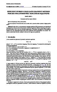
Intuitively, we would expect the Plan Modification Algorithm to perform better than the Plan Generation Algorithm in contexts in which agents are loosely-coupled, as few modifications would have to be made to the multiagent plan to resolve any plan flaws. To test our intuition, we compared the performance of the two algorithms on random problems drawn from the convoy domain described in Section 2. In order to produce randomly-generated convoy problems, we created a convoy grid world, in which agents start at particular vertices in the grid, and must construct plans to traverse the edges of the grid to arrive at their goal vertices. The edges have different properties that affect how the agents must traverse them, designed to create various possible plan interactions between agents, should their paths overlap. The edges allow for 29
both positive and negative interactions, as well as interactions that involve both temporary and permanent changes to the world-state. More details on the grid world, as well as formal operator specifications from which the corresponding agent plans were built, can be found in [6]. To create problem instances drawn from our convoy domain grid world, we created tenby-ten grids, where each edge’s properties were randomly drawn from the set of possible edge types. Then, each agent was given a randomly-generated path of length five (meaning that five edges were traversed) from an arbitrary starting point to an arbitrary ending point in the grid (though no agent’s path traversed the same edge more than once).2 Given this setup, we formalized the degree of coupling between agents in terms of the number e of pairs of overlapping edges traversed by the agents given their particular plans. Agents who are uncoupled have paths that do not overlap, and thus have no shared edges (e = 0). At the other extreme, agents whose plans are tightly coupled will have an e that scales linearly with the number of agents, making the complexity of our algorithms exponential. In contrast, agents who are loosely coupled will have an e that is a sublinear function of the number of agents. For each desired coupling case, we generated thirty random problems for numbers of agents from two to ten, and computed the median number of plan states (as well as the inter-quartile range, indicated by error bars in the graphs) generated by the PMA and PGA to find the optimal solution. Also, we terminated an algorithm run if it had generated at least a million plan states without returning the optimal solution, and used this number as a measure of the performance of the algorithm on the problem (hence the use of inter-quartile ranges instead of standard deviations in our measurements, as the former are less sensitive to such cutoff measurements). We tested the algorithms under a variety of coupling cases, where the coupling of the problem generated was determined by the number of overlapping pairs of edges. First, we tested the algorithms in the uncoupled case, where e = 0. The results of the uncoupled case are displayed in Figure 12 (note the logarithmic scale and interquartile range). We then tested the √ algorithms on a loosely coupled case, where e = 5n, and a tightly coupled case, where e = 2n, 2 The
reader will note that for these experiments we have fixed the length of the agents’ plans but varied the number of agents. If the agents’ plan lengths also varied, then the coupling function would have to incorporate the plan length as well. Our algorithm will in fact perform even better when what grows is agent plan length and not the number of agents, because longer, serial plans reduce the space of acceptable coordinated solutions (as the steps of the agents start with more ordering constraints between them and thus have fewer possible ordering adjustments).
30
where again n is the number of agents. The results are displayed in Figure 13 and Figure 14 respectively. PMA
PGA
1000
Visited States
100
10
1 0
2
4
6
8
10
12
Agents
Figure 12: Testing the PMA and the PGA on e = 0
Plan-Modification
Plan-Generation
10000
Visited States
1000
100
10
1 0
2
4
6
8
10
12
Agents
Figure 13: Testing the PMA and the PGA on e =
√ 5n
As expected, for loosely-coupled problems, the PMA continues to perform efficiently as the number of agents increases. The PMA outperforms the PGA especially well in the uncoupled case, where the PMA simply needs to identify that there are not any interactions, but where 31
Plan-Generation
Plan-Modification
1000000
100000
Visited States
10000
1000
100
10
1 0
1
2
3
4
5
6
7
8
9
Agents
Figure 14: Testing the PMA and the PGA on e = 2n PGA has to regenerate the uncoupled plans. However, the difference between the two becomes less obvious as the degree of coupling increases, as in Figure 14. These results show empirically the relative performance of each approach on loosely coupled benchmark problems, demonstrating the superior performance of the PMA over the PGA. As always, the particular algorithm appropriate to a coordination problem can vary, depending on the nature or structure of the problem. However, these results demonstrate the efficiency gains that can be achieved on loosely coupled Multiagent Plan Coordination Problems using our Plan Modification Algorithm that starts the search at a plan that is the union of the individual agent plans, rather than starting from an empty plan.
4.7
Comparisons to Other Approaches
Much of the earlier and foundational work on variants of the Multiagent Plan Coordination Problem shared a common approach, in that they concern themselves with the problem of temporal consistency before addressing possible flaws in the multiagent plan. For example, Yang’s approach [38] is to use a dynamic programming algorithm that considers all possible temporal alignments of the individual plans, and only handles flaws given a particular temporal alignment. Ephrati’s state-space search algorithm [12] operates in a similar manner, as the search works forward in time from the start of the agents’ plans to the fin32
ish, considering (in the worst case) all possible interleavings of the agent plans, and repairing flaws as they are discovered in the various possible interleavings. Mali’s SAT encoding [21] introduces SAT variables not only for the possible threats and causal links that could exist in the multiagent plan, but also for each plan step and every possible pairwise ordering between the steps. In all of these approaches, even if the agent plans are completely uncoupled, the algorithms will still search through a space of all possible plan orderings, a space that scales exponentially in the number of agents. In contrast, rather than worrying first or simultaneously about the temporal consistency of the coordinated plans, our Plan Modification Algorithm first addresses the flaws present in the multiagent plan (be they conflicts or redundancies) and only afterward verifies the temporal consistency of the resultant plan. In the limit, when there are no flaws in the set of agent plans to be coordinated, the PMA will terminate in the time it takes to verify this property, with a time complexity of O((dn)2 ), where n is the total number of agents and d is the number of steps in each agent’s plan. More generally, this characteristic is what makes the PMA responsive to the degree of coupling between the agents, resulting in tractable algorithmic performance when the agents’ plans are loosely coupled. 4.7.1
A Representative Comparison to Coordination as Satisfiability
In [6] and [7], we make analytical and empirical comparisons to several past approaches to coordination problems, such as those of Yang [38], Ephrati [12], and Mali [21], that illustrate the advantages of the PMA on loosely-coupled problems. To give the reader a sense of how our approach contrasts with other approaches that consider temporal consistency first or simultaneously, we here summarize our comparison to the approach taken by Mali [21], which casts the problem of plan coordination as a Satisfiability problem. In Mali’s work, he considers two possible plan encodings, a state-space and a plan-space (or causal) encoding, and establishes that causal encodings can be smaller (and thus faster to solve) than state-space encodings, especially because of their sensitivity to the degree of coupling between the individual plans. Because of this result, we compare our PMA against SAT algorithms run on his causal encoding. Mali’s causal SAT encoding of the plan coordination problem is based on Kautz’s grounded causal SAT encoding of the standard partial-order planning problem [16], but modified to re-
33
strict the solution space to only include steps in the original set of individual plans. For a given plan coordination problem M, Mali creates the following variables: 1. ∀Si ∈ S(M), create a variable si . (Create a variable for every plan step in the plan.) 2. ∀Si , S j ∈ S(M) create a variable si j . (Create a variable for every possible ordering between steps in the plan.) 3. ∀Si , S j ∈ S(M)|c ∈ pre(S j )andc ∈ post(si ) create a variable sic j . (Create a variable for every possible causal link between pairs of steps.) The clauses are specified as follows: 1. si j ⇒ (si ∧ s j ). (If an ordering constraint is present, so are the steps in the constraint.) 2. ¬sii . (A step cannot be ordered before itself.) 3. si j ∧ s jk ⇒ sik . (Enforce the transitivity of ordering constraints.) 4. ∀c ∈ pre(s j ), s j ⇒ ∀sic j (sic j1 , ∨... ∨ sic jn ). (If a step exists, its preconditions must be met by a causal link.) 5. si jn ⇒ si ∧ s j (If a causal link exists, so must the steps in the link.) 6. si jn ⇒ si j (A causal link implies an ordering constraint.) 7. ∀sk , ¬c ∈ post(sk ), sic j ⇒ ski ∧ s jk . (All causal-link conflicts must be resolved.) Although Mali casts the plan coordination problem as a Satisfiability problem and not an optimality problem, it is trivial to convert the SAT problem to a weighted MAXSAT problem [13], by assigning an infinite weight to all SAT clauses specified in the above encoding, and then creating a unit clause for each plan-step variable, each with a weight of one. This encoding will ensure that the solution found is the one with the fewest number of plan steps, subject to the hard constraints on the problem. Mali [21] conducts an analytic evaluation of the asymptotic complexity of his causal encoding of the plan coordination problem. Specifically, he shows that, given k plan steps and c step conditions, the number of variables in the SAT encoding will be on order O(k2 c). This 34
quadratic result stems from the fact that in the worst case we would have to consider all possible causal links between pairs of steps. However, Mali points out that the number could in fact be smaller if we take into account the conditions associated with each plan step, to rule out creating causal links between pairs of steps that either do not produce or do not require the condition associated with the link. Thus, the encoding is somewhat sensitive to the degree of coupling between the agent plans, unlike Yang’s approach [38]. However, a key element of his encoding prevents MAXSAT solvers from exploiting the loose coupling of the problem. This is that the SAT encoding introduces variables not only for possible causal links that could exist in the multiagent plan, but must also do so for each plan step and every possible pairwise ordering between the steps. In addition, SAT clauses are created between these edges to enforce the temporal consistency (acyclic property) of the plan. This sets Mali’s approach apart from our own, as we fold the (quadratic) cycle check inside the evaluation of a particular plan. In contrast, Mali forces the check to be conducted in the search space of possible satisfying assignments to variables, which means even for completely uncoupled problems, he will produce k3 clauses (the transitivity enforcement clauses) and at least k2 variables (each representing a possible ordering of a pair of steps). The implications of this are that even if the agent plans are completely uncoupled, a MAXSAT solver will have to rediscover valid temporal orderings between the steps in the agents’ plans, redoing all the temporal reasoning that was done by the individual agents. Obviously, this has a significant impact on the tractability of this approach to the Multiagent Plan Coordination Problem. When we compare the asymptotic complexity of the PMA to Mali’s approach, we see that, like Yang’s and Ephrati’s approaches, Mali’s is also insensitive to the degree of coupling between the plans of the agents. We explore the empirical implications of this fact when we experimentally compare Mali’s encoding to the PMA in the next subsection. 4.7.2
Empirical Comparisons
To empirically compare Mali’s encoding of the MPCP as a MAXSAT problem against our PMA, we compared the number of plan states visited by the PMA (as in Section 4.6.2) against the number of clauses required to produce the SAT encoding of the same problem. The rationale behind this comparison is that no MAXSAT algorithm, no matter how fast, can avoid having to set each variable and test each clause once, even if it can correctly guess an optimal 35
assignment of values to the variables. The computational cost of verifying a SAT clause is comparable to the creation of a plan state by fixing a plan flaw, since the latter involves only a small number of adjustments to the original plan state (adding an ordering constraint or causal link, or removing a plan step). Furthermore, all SAT solvers have a worst-case complexity that is exponential in the number of (unique) clauses in a SAT problem, and a best case complexity that is linear in the number of these clauses. In this sense, the number of clauses serves as an effective lower bound on the performance of any MAXSAT solver. Thus, we are in fact comparing the time needed for our algorithm to solve the MPCP against the time needed for Mali’s
Algorithmic Effort
method to simply encode the MPCP so that it can be solved by a SAT solver.
Figure 15: Plan-Modification Algorithm vs. Mali’s SAT Encoding Again, we created random grid problems in the same way that they were created previously, √ where the number of pairs of overlapping edges was e = 5n (where n is the number of agents). For each number of agents from two to ten, we generated thirty random problems, and computed the median number of states generated by the PMA and the median number of clauses 36
generated by the SAT encoding (as well as the inter-quartile range, shown with the error bars). The results are shown in Figure 15 (note the logarithmic scale). The graph shows the problem with using Mali’s SAT encoding to solve even loosely coupled Multiagent Plan Coordination Problems, because of the implementation of the enforcement of transitive closure in the space of SAT variable assignments. This empirical result is consistent with Mali’s own complexity analysis.3 As we have indicated, the complexity of Mali’s method is independent of the degree of coupling of the agents. This is because the number of clauses that he must introduce is almost entirely a function of the number of plan steps across the set of agent plans, irrespective of how those plan steps interact. This means that the results shown for Figure 15 must also hold for any other degree of coupling between the agents in the MPCP. In contrast, as we have shown previously in Section 4.6.2, the performance of the PMA very much depends on the degree of coupling. Although we have not demonstrated it empirically, it is not hard to imagine a “crossover point” at which the degree of coupling in an MPCP becomes tight enough to cause the number of clauses Mali must generate to be exceeded by the number of plan states the PMA must generate to solve it. However, it is likely that the PMA would still outperform Mali’s method even in these cases, as a SAT algorithm would still need to solve the problem created by Mali’s encoding, possibly using time exponential to the number of problem clauses.
4.8
Summary
In this section, we have formally defined the Multiagent Plan Coordination Problem (MPCP), described algorithmic techniques for solving it via modification (PMA) and via generation (PGA), and have shown that, while the worst-case complexity of any algorithm is still exponential, the PMA technique using appropriate heuristics can perform well in the expected case. We further delved into a comparison between the PMA technique and a representative prior technique done by Mali to not only show that our approach performs much better on loosely3 Note
that comparing the number of plan states to clauses gives a flavor of the computational effort, but does not account for computational time needed for creating each of these respectively. If clauses could be created three orders of magnitude faster than plan states, for example, then the computational effort of the curves in the graph would be comparable. However, because clause generation, in our experience, is not that much faster, and because the data for Mali’s approach includes encoding but not solving effort, we believe that this graph effectively captures the qualitative relationship between the costs of the two approaches.
37
coupled multiagent planning problems, but also to explain why this is so in terms of how our approach orders the search process for finding and resolving coordination flaws between plans. There is clearly more that can be done in this area, as we outline for our future work (Section 6). Of particular interest would be to figure out how to compare our approach to that of Chen et al. [37]. A fundamental challenge in conducting such a comparison would be in deciding on the space of multiagent problems that is appropriate for comparison, and how those problems are expressed. If the problems inherently assign the agents loosely-coupled problems, then that obviates the need for finding effective decompositions, which is the strength of Chen et al.’s approach. If problems are not well decomposed initially, on the other hand, then Chen et al. should perform well assuming that agents are willing to accept arbitrary subproblems from a centralized decomposition process. In short, the work of Chen et al. is the state of the art in single-agent plan-merging technology, and as we (and others) have pointed out there are significant similarities between plan-merging and plan-coordination. But there are fundamental differences in the assumptions behind these different research areas that would need to be reconciled between the communities before a meaningful comparison could be done.
5
A Distributed Framework for Solving the Multiagent Plan Coordination Problem
So far, the coordination algorithms we have described have been assumed to execute in a centralized manner, where a single agent collects the decentrally formed plans of different agents, constructs the MPCP, and then solves it, disseminating the coordinated solution to the group. Although there is nothing inherent in our algorithms that requires them to be run centrally, we did not specify any protocol to allow agents to solve the problem in a distributed or parallel manner. Since the Multiagent Plan Coordination Problem is fundamentally a multiagent problem, it is natural to think about ways of utilizing multiple agents to construct and solve the coordination problem together, rather than arbitrarily relying on a single agent to carry out the task alone. Although there are a variety of reasons why problems are solved in a distributed manner, such as privacy and fault tolerance, the advantage that is most relevant to this work is that by distributing
38
the coordination process, we can take advantage of the parallel computational resources of all of the agents whose plans are being coordinated. To formulate a decentralized approach to the MPCP, we capitalize on existing distributed systems work by showing how the problem can be cast as a Distributed Constraint Optimization Problem (DCOP). We map the decentralized MPCP into a DCOP, where coordination flaws and planning choices (such as conflicts, steps, and causal links) are treated as variables, where flaw repairs or planning decisions are the possible values that the variables can take on, and where temporal and causal relationships between actions impose constraints on legal flaw repair combinations. We can then exploit previously-developed fast and powerful techniques for solving DCOPs. Specifically, in this section we make use of ADOPT, a distributed constraint optimization framework developed by Modi et al. [23]. To use ADOPT to solve the MPCP, we first describe a transformation of the Multiagent Plan Coordination Problem to a Constraint Optimization Problem. We then introduce a new strategy for solving the Multiagent Plan Coordination Problem within the DCOP framework through an innovative blending of general-purpose DCOP techniques (such as exploiting problem locality) and our Plan Modification Algorithm. We then compare the use of the ADOPT framework to solve the MPCP with our Plan Modification Algorithm running in a stand-alone centralized mode, showing that despite the advantage of parallel processing, solving the MPCP using ADOPT is generally not any faster than using our PMA in a centralized manner. We note that the work described in this section is an extension of our previously published work [8].
5.1
Encoding the MPCP as a COP
The key advantage of a distributed constraint optimization framework like ADOPT [23] is how such a framework allows multiple agents to solve a constraint optimization problem (COP) concurrently. In order to use such a framework, we first illustrate how we can cast the MPCP as a COP. A constraint optimization problem consists of n variables x1 , x2 , ..., xn , where the possible values of each variable are drawn from a set of discrete domains D1 , D2 , ..., Dn . The goal of the problem is to find an assignment of values to variables that minimizes the global cost function over the set of variables. The global cost function is computed by aggregating the costs of the violated constraints in the problem.
39
Given our previous description of the MPCP, we can cast the MPCP as a COP, where the optimal plan is one that has a minimal aggregate step cost, subject to the constraints that all conflict flaws are resolved, and that the plan is acyclic. To ease exposition, we make continual reference to Figure 16, which represents a simplified version of the convoy problem from Section 2. In the figure, the two plans share a redundant Clear Block step, but have no causal-link conflicts (the Initial State steps and Goal steps of the agents have been joined to simplify exposition). The COP representation of this MPCP is illustrated in Figure 17, where each variable is given a number corresponding to the step or causal link it represents in Figure 16. The domains of the variables are specified in brackets, below the variable. The variables in bold are step variables. The edges between variables represent constraints, and the tuples that appear on the edges represent assignments to the variables that violate the constraints. ) ) (7 A1 , k c blo At( At (b lo ck ,A 2) (1 0)
Initial State (1)
Clear Block (2)
Cleared(block) (8)
Clear Block (5)
Move To Goal (3)
at( go al, A
) (12 A1) al, o g ( at
Move To Goal (6)
Cleared(block) (11)
1) (9)
Goal (4)
Figure 16: Example Coordination Problem
(a, p)
8
(a, 3)
3
{2, 5, a}
{p, a}
9
{3, a}
p) (a,
{p}
{p, a}
{1, a}
(a ,1 )
(a, 2)
) ,2 (a
1
1) (a,
2
(a ,5 )
(a, p)
7
, (a (a, p)
10
{1, a}
5
(a, 5)
11
{p, a}
(a, p)
6
{2, 5, a}
(a, 6)
{p, a}
p)
4
{p}
12
{6, a}
Figure 17: Matching COP
5.2
Specifying Variables
We convert a MPCP to a COP in the following way. Given a multiagent plan coordination problem M, we create a variable for each possible precondition pre of each plan step s, for each possible plan step s, and for each possible causal link conflict flaw t. To create the COP, for each plan step, we create a variable with a domain of {p, a}, as the step can either be 40
present or absent from the plan (the only exception are init and goal steps, which each have a singleton domain of {p}, as such steps cannot be removed from the plan). In Figure 17, there are variables for steps 1 through 6, each with binary domains, except the variables 1 and 4, which represent the initial state and goal steps, respectively. For each precondition pre of each step s, we create a variable with a domain hs1 , ..., sn , ai, where n is the number of steps that could establish the precondition pre to form a causal link (the domain represents the set of step variables that achieve pre, as well as the possibility that the causal link is absent from the plan). In Figure 17, the links are represented by variables 7, 8, 9, 10, 11, and 12. The causal link variables all have binary domains, except for 8 and 11, as they represent the establishment of the condition Cleared(Block), which can be established by either step 2 or 5. Finally, for a causal-link threat flaw t = hsa , sb , sc i (meaning step sc threatens a possible link between sa and sb ), we create a domain of size three ({i, p, d}), where i corresponds to the threat being ignored, p corresponds to the threat being resolved by promoting the clobbering step before the link, and d corresponds to demoting the clobbering step after the link. Note that the threat can be ignored and a solution is still possible if either step involved in the causal link, or the clobbering step itself, is absent from the plan.
5.3
Constructing Variable Constraints
The relations between flaw variables are specified by constraints over the variables. We describe the constraints between flaw variables by indicating the no-good sets between the variables, that is, combinations of values that the connected variables cannot take. For example, a binary constraint between variables vi and v j can be described by a set h(0, 1), (1, 0)i, meaning that the constraint prevents variables vi and v j from being assigned values 0 and 1, or 1 and 0 respectively. To illustrate the constraints, we again make reference to the MPCP in Figure 16, as well as the corresponding COP in Figure 17.
The necessary and sufficient constraints on the COP follow naturally from this encoding and an understanding of the MPCP, and are specified as follows:
41
An All Preconditions Satisfied constraint ensures that all of a step’s preconditions are met if the step is in the plan. Formally, for a step variable s, for each causal link variable pre representing a precondition of s, we create a binary constraint c = h(a, p)i. There are many of these constraints, one example being the constraint between variable 7 (the link establishing the condition at(block, A1)), and variable 2 (step Clear Block), as a step cannot be present if one of its preconditions is not met. A Constrain Step Removal constraint ensures that a step being used to achieve a precondition of another step remains in the plan. Formally, given a causal-link variable l, for each step variable s that could establish the causal-link’s condition, we create a binary constraint c = h(si , a)i, where si is the index of step s in the link’s domain. This constraint prevents step s from being removed if it is being used to establish the link. There are many of these constraints, one example being the {a, 2} constraint between variable 2 (step Clear Block) and causal link variable 8 (the link establishing the condition cleared(block) for step Move to Goal). This constraint prevents Clear Block from being absent (a) if the link is using it (2). A Reward Step Removal constraint ensures that the minimum cost plan will be generated. For a variable s representing a plan step, we add a unary constraint h(p)i. Note that, in general, all redundant steps cannot be eliminated, so these unary constraints will tend to over-constrain the problem. This is a motivation for doing constraint optimization, instead of constraint satisfaction. The cost of each constraint depends on the cost of the step it represents. To keep Figure 17 uncluttered, the unary constraints are not shown in the figure. A Handle Threats constraint ensures that a threat flaw is handled either by ordering the steps, or by removing any of the three steps involved in the threat. For a variable t representing a threatening step sc to causal link l between steps sa and sb , we add a constraint c between the threat variable, the causal link variable that has l as a possible value, and the variables representing the steps, where c = h(i, l, sa , sb , sc )i. Since there are no threat variables in the example MPCP, there are none of these constraints in Figure 17. A Temporal Consistency constraint ensures that the multiagent coordinated plan remains acyclic in terms of the temporal constraints over the steps in the plan. Unlike the previous constraints, which can be generated in polynomial time, is not computationally feasible to explicitly enumerate all possible no-goods for a Temporal Consistency constraint (and thus they are not captured in Figure 17), but the constraint can be checked by implementing possible flaw 42
resolutions in the temporal network representing the agents’ plans, and checking the resultant network for cycles, which can be done in O(n2 ) time. This, in effect, is how we will test this constraint in the COP encoding of a MPCP. Finally, because (as we describe next) the same variables could be assigned to different agents, we introduce one more constraint on the DCOP, a Variable Assignment Consistency constraint that requires that different agents assign the same value to the same DCOP variable. In our work, we assume that agents require consistent plans (meaning acyclic plans without any causal-link threat flaws), but also want plans that have the lowest aggregate step cost. To produce this, we make the cost of violating all constraints except the Reward Step Removal Constraint infinite, as such violations will result in inconsistent plans. The cost of violating a unary Reward Step Removal Constraint is the cost of the step that the constraint holds over.
5.4
Using ADOPT for Distributed Multiagent Plan Coordination
To test whether our encoding of the MPCP into DCOP faithfully captures the problem, we wanted to use the encoding in an existing, off-the-shelf DCOP framework. Such frameworks enable agents to converge on a globally consistent solution to a DCOP in a distributed manner. Since a variety of alternative frameworks exist [23, 20, 26], any of which could serve to test of whether our encoding method yields a solvable DCOP, we chose the DCOP framework called ADOPT, developed by Modi et al. [23] because we were most familiar with its implementation and use. Some of the features of ADOPT include the ability to optimize a global function via local communication, the ability for agents to compute their variable values in an asynchronous manner, and the ability to provide quality guarantees so that trade-offs between solution quality and computation time can be considered. A straightforward way of using ADOPT to solve the MPCP is to convert the MPCP into a COP using our COP transformation described previously, and then create an ADOPT agent for each COP variable. The ADOPT agents then use the constraints and the ADOPT protocols to converge on a globally optimal solution. One obvious problem with this formulation is the fact that the MPCP involves an existing set of agents, and so it does not make sense to think of “creating” ADOPT agents. Modi et al. [23] indicate how to address this concern by allocating
43
to each agent a set of variables, and then combining the set of variables into a single variable with a domain that is the cross-product of the domains of the original variables. However, this approach does not address how agents are assigned these sets of variables. The strategy we use is one that attempts to exploit problem locality, by having agents take responsibility for the flaws that involve their own associated plans. Assigning variables along the lines of the original plans builds on our previous results [8], in which a locality-based variable assignment strategy worked better than a purely load-balanced one. Such an assignment could leave an agent with more variables than others, but this is outweighed by the advantage of being able to reason locally about interacting variables. Giving a single agent that is disproportionately involved in more flaws responsibility for resolving them can be viewed as a form of partial centralization along the lines of work by Mailler [20]. It may be possible to exploit both problem locality and load balancing as well, but such strategies are beyond the scope of this paper. Since flaws by definition can involve more than one agent’s plan, when assigning a causal link variable, the agent who is the consumer of the link takes responsibility for the flaw. For threat flaw variables, the agent whose step threatens the link takes responsibility for the variable. Finally, for each flaw variable that an agent takes responsibility for, it also takes responsibility for the variables of the steps involved in the flaw (hence the need for the Variable Assignment Consistency Constraints, as step variables are thus assigned to more than one agent). A key benefit of this locality-based flaw distribution is that flaws that involve the same plans are more likely to interact with each other via the problem constraints. Thus, rather than having to create a domain of values representing the cross-product of all assigned variables, an agent can apply the COP constraints to possible values of this cross-product to eliminate locally bad values, before coordinating with other agents. To make this elimination process more efficient, we embed a local copy of our Plan Modification Algorithm inside each agent. The agent then runs the PMA on its set of flaws with the bounding mechanism disabled, recording all consistent (i.e., finite-cost) solutions found. This consistent set now represents its variable domain. Figure 18 illustrates how the agents divvy up the flaw variables from the DCOP in Figure 17, using the previously specified flaw-assignment strategy. The top eight variables belong to the first agent, and the bottom eight eight variables belong to the second agent. Besides 44
assuming control of all flaw variables just involving its individual plan, the first agent has taken responsibility for link variable 8, as well as the lower agent’s step variable 5. The second agent’s variable assignments mirror those of the first agent. Note the Variable Consistency Constraints between the shared variables, 2 and 5, ensuring that the agents agree on the presence of absence of the corresponding steps in the plan. (a, p)
{p}
)
{p, a}
9
{3, a}
4
2 (a ,2 )
)>
(a ,1 )
{2, 5, a}
(a, 6)
3
5
p a, ,( a) p,