Efficient Compilation Techniques for Large Scale Feature Models Marcilio Mendonca1 , Andrzej Wasowski2 , Krzysztof Czarnecki1 and Donald Cowan1 University of Waterloo1 , IT University of Copenhagen2 {marcilio,dcowan}@csg.uwaterloo.ca,
[email protected], and
[email protected]
Abstract Feature modeling is used in generative programming and software product-line engineering to capture the common and variable properties of programs within an application domain. The translation of feature models to propositional logics enabled the use of reasoning systems, such as BDD engines, for the analysis and transformation of such models and interactive configurations. Unfortunately, the size of a BDD structure is highly sensitive to the variable ordering used in its construction and an inappropriately chosen ordering may prevent the translation of a feature model into a BDD representation of a tractable size. Finding an optimal order is NP-hard and has for long been addressed by using heuristics. We review existing general heuristics and heuristics from the hardware circuits domain and experimentally show that they are not effective in reducing the size of BDDs produced from feature models. Based on that analysis we introduce two new heuristics for compiling feature models to BDDs. We demonstrate the effectiveness of these heuristics using publicly available and automatically generated models. Our results are directly applicable in construction of feature modeling tools. Categories and Subject Descriptors D.2.2 [Software Engineering]: Design Tools and Techniques—Computer-aided software engineering (CASE) General Terms Design Keywords Model-driven development, software-product lines, formal verification, Configuration, feature modeling
1. Introduction Generators and components support the creation of systems within system families. A system family is a set of systems
Permission to make digital or hard copies of all or part of this work for personal or classroom use is granted without fee provided that copies are not made or distributed for profit or commercial advantage and that copies bear this notice and the full citation on the first page. To copy otherwise, to republish, to post on servers or to redistribute to lists, requires prior specific permission and/or a fee. GPCE’08, October 19–23, 2008, Nashville, Tennessee, USA. c 2008 ACM 978-1-60558-267-2/08/10. . . $5.00 Copyright °
sharing enough common properties to warrant basing their development on a common set of reusable assets, such as frameworks, components, and generators. Building such assets requires understanding both the common features and the varying features of systems within a family. For example, all e-commerce systems are likely to provide common features such as catalog browsing and product checkout. However, the systems may differ in several respects, e.g., whether they support selling physical products or electronic products or both and whether they allow guest or registered checkout or both. Feature modeling is a technique for representing the common and variable features of systems in a system family. A feature model is a hierarchy of mandatory, optional, and alternative features with possibly additional constraints, such as implications between pairs of features [19]. Feature modeling is used in system family scoping, i.e., deciding which features should be supported by the common assets and which not, identifying architectural variation points, and in system configuration [10]. Feature models can directly represent a class of domain-specific languages that are focused on configuration. Systems can be specified as configurations of features and such specifications can be used as input to code generators, e.g., [14], or to configure requirements and design models [12] or components [6]. Feature models have been semantically related to propositional logic [5, 13]. The translation of feature models into logic representations has allowed the use of reasoning tools for automated feature model analyses [4], such as consistency checks and finding dead features, refactoring [2], reverse engineering [13], and interactive configuration [25]. All of these applications require an efficient representation of the configuration space of the features. Binary Decision Diagrams (BDDs) [9, 22] are one such representation, which supports efficient logical tests and interactive guidance algorithms [18]. Interactive configuration is a process of selecting a particular variant out of those represented by a model. The process is interactive since it includes user steps, such as selecting and eliminating features, and the machine responses, such as selecting implied features and excluding incompatible features. The interactive guidance in this context is provided by calculating so-called valid domains, i.e., possible assignments of features given the current state of the
Legend
r a
b [1, 1]
a1
b1
b2
b3
Constraint-1: a1 → b3
f
Mandatory feature
f
Optional feature
f
Grouped feature Feature group with cardinality [1, 1]
Figure 1: A feature model system, and propagating information whenever new choices are made. Efficiency is extremely important for some of the above applications, in particular for detecting refactoring opportunities and for interactive configuration. These two are normally performed as a part of each interaction and thus should guarantee response times within milliseconds. Since the response time of most of standard algorithms on BDDs requires time proportional to the size of the BDD [3], it is desirable to devise technologies that can decrease this size as much as possible. One such approach is a topic of our present paper. Each BDD has a fixed variable ordering associated. This ordering has a dominant influence on its size. A bad order can be seriously detrimental leading to excessive memory use, often beyond capabilities of typical workstations. On the other hand a very good order can dramatically compress the BDDs (down to kilobytes!), enabling extremely fast processing with interactive algorithms. It is thus natural that quite a few researchers in various domains have investigated the ordering minimization problem. In this paper, we approach this problem by proposing efficient ordering heuristics for the feature modeling domain. Experimental results show that the proposed heuristics allow for efficient compilations of feature models with up to 2,000 features. We proceed with Section 2 providing a short background on feature models, and Section 3 introducing the variable ordering problem. State-of-the-art solutions are reported in Section 4. Section 5 documents design decisions in choosing a new reordering heuristics for feature models, followed by Section 6 presenting the heuristics, experimental analysis (Section 7) and conclusion (Section 8).
2.
Feature Models
A feature model consists of (i) a feature tree and (ii) possibly one or more extra constraints, which are propositional formulas over features. Fig. 1 depicts a sample feature model. Its feature tree (top left) has a root feature r, mandatory features b and b1 , optional features a, and a1 , and an exclusiveOR group containing grouped features b2 and b3 . The implication a1 → b3 labeled Constraint-1 is the extra constraint. A feature model denotes a set of legal configurations. A legal configuration is a set of features selected from the feature model according to its semantics. The set of legal
configurations is given by a conjunction of the extra constraints with a propositional formula that is systematically constructed from the feature tree [5, 13]. The formula is a conjunction of (i) the root feature, (ii) an implication from each child feature to its parent, (iii) an implication from each feature with a mandatory child to that child, (iv) an implication from a parent with an inclusive-OR (exclusive-OR) group to a disjunction (pairwise mutual exclusion) of the group members. Applying this derivation to the sample feature tree in Fig. 1 yields, after some simplifications, the formula r ∧ b ∧ b1 ∧ (a1 → a) ∧ (b → b2 xor b3 ). Next, we provide definitions that are used throughout the paper: D EFINITION 1. The extra constraint representativeness (ECR) is the ratio of the number of variables in the extra constraints (repeated variables counted once) to the number of variables in the feature tree. ECR for the feature model in Fig. 1 equals
2 7
' 0.28.
D EFINITION 2. For features f1 , ..., fn their lowest common ancestor, written LCA(f1 , . . . , fn ), is their shared ancestor that is located farthest from the root (where a feature is an anscestor of itself). For features of Constraint-1 we have LCA(a1 , b3 ) = r. D EFINITION 3. Given f = LCA(f1 , . . . , fn ), the roots of features f1 , ...,fn , written Roots(f1 , . . . , fn ), is either the set {f}, if f has no children, or the subset of f’s children that are ancestors of f1 , ..., fn . In our example Roots(a1 , b3 ) = {a, b}, since features a and b root the subtrees containing a1 and b3 respectively.
3. BDDs and The Variable Ordering Problem decision diagram (BDD) [9, 3] is a concise representation of a Boolean function. BDDs are directed acyclic graphs (DAGs) having exactly two external nodes representing constant functions 0 and 1, and multiple internal nodes labeled by variables. For instance, Fig. 2a depicts a BDD for formula (a → b). Each internal node has exactly two outgoing edges representing a decision based on an assignment to the node variable: the low-edge (a dotted line in the figures) represents the choice of false, while the high-edge (solid) represents the choice of true. A path from the root to an external node represents an assignment of values to variables. For example the rightmost path in Fig. 2a represents a (non-satisfying) assignment [ a 7→ 1, b 7→ 0 ]. The paths terminating in the external node 1 (respectively 0) represent satisfying (respectively unsatisfying) assignments. A BDD is ordered if every top-down path in the DAG visits the variables in the same order. In a reduced BDD any two nodes differ either by labels or at least by one of their children (uniqueness), and no node has both edges pointing to the same child (non-redundancy). Notice that the three
a1
r
b1
b1
b1
b
b3
b2
a
b
b3
b3
b3
b
r
a
b
r
r
a
b b2
a1
1
0
Variable order: (a) a < b
0
b2
1
1
(b) r < b1 < b < b2 < b3 < a < a1
0
(c) a1 < b1 < b3 < b < r < a < b2
Figure 2: (a) A simple BDD; (b-c) BDDs for the model in Fig. 1 with two different variable orders BDDs in Fig. 2 are both reduced and ordered. We shall use the term BDD as a synonym for ROBDDs from now on. During the last two decades BDDs have been widely applied to address large scale combinatorial problems in logic synthesis, verification, configuration, constraint satisfaction and optimization. Off-the-shelf BDD libraries are freely available (e.g. JavaBDD, Buddy, CUDD). What makes BDDs so appealing is polynomial time algorithms for applying Boolean connectives and constant time satisfiability and equivalence checks (recall that these are generally NPhard). Crucially for configuration, polynomial algorithms for computing valid domains are known [16, 17]. Fig. 2b presents a BDD for the formula r ∧ b ∧ b1 ∧ (a1 → a) ∧ (b → b2 xor b3 ) ∧ (a1 → b3 ), which corresponds to the model of Fig. 1. The BDD contains 8 internal nodes, 2 external nodes, and 3 satisfying paths, each representing one or more solutions. A major drawback of BDDs is their high sensitivity to variable ordering. For an illustration of the problem, consider the BDD in Fig. 2c representing the same formula as Fig. 2b, but with another order. While the original BDD (Fig. 2b) had only 10 nodes, the new one contains as much as 16 nodes—60% more! In the worst case this difference is exponential, which can translate to millions of nodes in practical applications. Unfortunately, finding an optimal variable order, which minimizes the size of a BDD, is an NP-hard problem [7, 22]. For this reason it is typically approached by heuristic algorithms. Heuristics exploit specifics of the problem domain in order to compute good orders efficiently. Typically research communities applying BDDs develop such heuristics for their domain. In this paper we investigate the problem for the feature modeling domain, with the goal of
enabling BDD-based feature modeling tools to handle very large models.
4. A Survey of Variable Ordering Heuristics A pervasive goal of all the ordering heuristics is placing variables that are combinatorically related close to each other in the ordering. This task is nontrivial. Dependencies between variables often interfere: optimizing the placement of a variable with respect to one dependency often decreases the quality of the ordering with respect to the others. Variable ordering heuristics can be categorized into dynamic and static. Dynamic heuristics reorder the variables on-the-fly during construction and manipulation of a BDD, usually exploiting library’s garbage collection cycles. Static heuristics compute a variable order off-line, which is then applied once to construct and analyze the BDD. 4.1 Static Heuristics BDDs have been very successful in synthesis and analysis of digital circuits. Similarly to a BDD, a circuit represents a Boolean function, and there exist direct translations between circuits and BDDs in either direction. Since the efficiency of verification strongly depends on the size of the BDD used, it is not surprising that the variable ordering problem has been deeply studied for the circuit domain. Feature models can be easily translated to Boolean circuits, which enables the use of existing ordering heuristics from that domain. Since Boolean connectives directly correspond to gates of the circuit, one can translate feature models in a syntax directed way. We have implemented this translation to basic circuits with AND, OR, and NOT gates and evaluated the usefulness of circuit heuristics described below for the compilation of feature diagrams. The translation
is linear for all the feature model elements except for xorgroups, for which is it is quadratic in the size of the group. In our evaluations, the translation produced circuits 3 to 10 times larger than the corresponding feature model. Fujita’s Heuristic. Fujita-DFS [15] is a heuristic that traverses the circuit from the output to the inputs (which correspond to variables) in a depth-first search (DFS) order. During the traversal, inputs connected to two or more gates are placed first in the generated variable ordering in the hope that the remaining nodes in the circuit will form a tree-like structure for which a standard DFS produces good variable orderings. Since a circuit is a directed-acyclic graph (DAG) with a single output, if nodes connected to many other nodes are removed from such a rooted DAG, the remaining structure approximates a tree. Fujita-DFS proved to generate good orderings for some circuit benchmarks, e.g. ICAS-85 [8]. Level Heuristic. The level heuristic [21] assigns the depth level to each circuit node, which is the length of the longest path from that node to the output. Subsequently, the inputs are sorted in decreasing order of levels to produce the final order. The level heuristic performs particularly well for multi-level circuits in which the outputs of a sub-network serve as inputs to the next subnetwork in the chain. FORCE Heuristic. FORCE [1] is a domain-independent static heuristic for variable ordering. The heuristic is applied to a CNF formula and uses a measure called span to assess quality of placement for related variables. Given a pair of variables its span is defined to be their distance in a given variable ordering. The span of a clause is the maximum span of all pairs of variables occurring in the clause. Finally, the span of a CNF formula is the sum of spans of all its clauses. FORCE begins with a random variable ordering and through successive steps attempts to minimize the formula span by moving variables near each other. At each iteration a new order is produced, which serves as input for the next iteration. It stops when the span value no longer decreases. In order to apply FORCE, we implemented a simple CNF translation algorithm that traverses the feature tree in DFS and generates CNF clauses for each parent-child and feature group relation, as described in Section 2. 4.2 Sifting Sifting [26, 22] is a popular domain-independent dynamic heuristic implemented in most BDD libraries. Unlike a static heuristic, sifting operates dynamically by trying to reduce the size of an already existing BDD on demand or on-thefly; for example during garbage collection cycles. The main advantage of sifting is that it can enable the construction of BDDs that cannot be built with static heuristics. Sifting is a local search algorithm. It swaps variables in the BDD if this leads to an improvement of the BDD size. Despite its merits, sifting has a serious drawback. The heuristic can be extremely slow in practice. In fact, we observed running times of over an hour for tasks that could be
performed in a few minutes by good static heuristics. This is primarily caused by the fact that unlike FORCE a swap in a variable ordering requires a modification of the existing BDD to obey the new ordering.
5. Variable Orders & Feature Models Many heuristics adopt the rationale of identifying and shortening the distance of dependent variables as a means to produce good variable orders. For instance, in the Level heuristic connected variables share the same level in the circuit. Fujita’s heuristic uses a DFS traversal to identify connected variables in a circuit. As we mentioned before, span is the measure used by FORCE to approximate connected variables in a CNF formula. Based on this observation, we characterize the problem of ordering BDD variables in our domain as the problem of identifying related variables in feature models and producing variable orders that minimize the relative distance of such variables. What makes the problem particularly challenging is the fact that the relations in the extra constraints usually connect independent branches in the feature tree. This causes good orders for the feature tree to be extremely inefficient for the extra constraints, and vice-versa. In addition, the larger the ECR (see Definition 1 in Section 2) of a feature model the harder is to find a good order that suits both the feature tree and the extra constraints. One way of obtaining an ordering heuristic is to compile a feature model into an intermediate representation such as a CNF formula or a circuit and use available heuristics to process the ordering. However, this approach would completely ignore the domain knowledge. For instance, the variables in the feature tree are arranged hierarchically in a tree, for which simple traversals produce good orders. At the same time, as will be seen later, such arrangements are obscured in a CNF or circuit representation, which prevents the respective heuristics from exploiting them. Given the BDD variable ordering problem in configuration, we pose the following hypothesis: A significant reduction in the size and construction time of BDDs representing feature models can be achieved if the structural characteristics of the models are exploited to order the BDD variables. In the following, we consider factors that influence development of new heuristics for variable ordering in the feature
Figure 3: Feature P and children A, B, C, D
R
A
P
C
B
A
C
B
A
R
R
D
P
C
P
D
0
(a) Pre-order
D
R
1
1
0
(b) Post-order
P
B
0
1
(c) Average-order
Figure 4: BDDs for various traversals of the feature tree modeling domain. These considerations are then exploited in the next section when we propose such heuristics. Structure of relations in the feature tree is explicit. The feature tree defines the variables in the feature model and specifies most of its relations. Hence, good orderings for the feature tree are generally effective for the feature model. Since relations in the feature tree are well-known and follow a hierarchical arrangement, compact structural patterns can be identified for BDDs using simple traversal algorithms. Mandatory features disturb the analysis. Feature models allow the specification of mandatory features which might improve system family documentation but play no role in variability analysis. Mandatory features can be eliminated from the analysis as they represent binary bi-implications and hence can be automatically inferred from other features. A simplification algorithm safely removes mandatory features from the feature tree and updates all references to such features both in the feature tree and in the extra constraints, while preserving the core semantics of the model. The reduction of the number of features in a feature model can significantly reduce the size of BDDs since each feature potentially corresponds to multiple BDD nodes. Parent-child relations define the connected variables. Feature tree constraints are expressed in terms of ancestral relations and groups. Our experiments have revealed that minimizing the distance between sibling features in groups does not improve BDD sizes. Therefore, we only consider parentchild relations to identify connected variables. Fig. 3 shows an example of four parent-child relationships involving a feature P and its children A, B, C, and D. Since all five features are optional, relations R1, R2, R3 and R4 represent binary implications (child → parent). The goal of a good heuristic for the feature tree should be to minimize
the relative distance between P and each of its children in the variable order produced. Excessive minimization in one branch of the tree might cause poor minimization in others. For instance, one might decide to order variables P, A, B, C, and D in a straight sequence. However, by doing so features B, C and D are placed in between A and its children increasing their relative distance. In fact, if this strategy is applied recursively in the feature tree, BFS traversal of the feature tree is implemented, which is an extremely poor ordering. Pre-order produces good BDD patterns. DFS traversals produce good variable orders for feature trees. However, much can be done in terms of minimizing the distance between parent and children features than pre-order. For instance, a better approach would be to place the parent node in an average distance to its children. Surprisingly, this produces BDDs with chaotic structures that in many cases are larger than one expects. We observed that the placement of parents prior (pre-order) or after (post-order) their children often produced compact BDD structures. Fig. 4 shows three BDDs for features Root, P, A, B, C and D from Fig. 3. A variable order for a pre-order traversal of the feature tree is shown in Fig. 4a (R indicates the root feature). A BDD of size 6 is shown and a very compact structure is observed for pre-order, e.g., if P is true the BDD evaluates to true no matter the values of its children. Conversely, if P is false, whenever A, B, C, or D are true, the BDD evaluates to false. Postorder also produces compact patterns (Fig. 4b); however, the BDD structure contains a much higher number of paths to the one terminal. If P is placed between its children and R is placed near P (referred to as average-order in Fig. 4c) the size of the BDD increases to 8 nodes even though the relative distance between P and its children is reduced. Thus, we adopt pre-order as the reference variable ordering imple-
(a) Natural Pre-order
(b) Sorted Pre-order
(c) Clustered Pre-order
Figure 5: Three different arrangements for child features A, B, C, D, E, and F
Table 1: Variable distances for pre-order-based traversals of the feature tree
Feature Tree Traversals
Variable Order
Natural Pre-Order Sorted Pre-Order Clustered Pre-Order
P