compositing phase, in a sort-last parallel volume rendering system as shown in ..... we generate the run-length codes to index the blank and non-blank pixels.
Efficient Compositing Methods for the Sort-Last-Sparse Parallel Volume Rendering System on Distributed Memory Multicomputers
Don-Lin Yang, Jen-Chih Yu, and Yeh-Ching Chung1 Department of Information Engineering Feng Chia University, Taichung, Taiwan 407 TEL: 886-4-451-7250x3700 FAX: 886-4-451-6101 E-mail: {dlyang, jcyu, ychung}@fcu.edu.tw Abstract In the sort-last-sparse parallel volume rendering system on distributed memory multicomputers, as the number of processors increases, in the rendering phase, we can get a good speedup because each processor renders images locally without communicating with other processors. However, in the compositing phase, a processor has to exchange local images with other processors. When the number of processors is over a threshold, the image compositing time becomes a bottleneck. In this paper, we proposed three compositing methods, the binary-swap with bounding rectangle method, the binary-swap with run-length encoding and static loadbalancing method, and the binary-swap with bounding rectangle and run-length encoding method, to efficiently reduce the compositing time in the sort-last-sparse parallel volume rendering system on distributed memory multicomputers. The proposed methods were implemented on an SP2 parallel machine along with the binary-swap compositing method. The experimental results show that the binary-swap with bounding rectangle and run-length encoding method has the best performance among the four methods.
1. Introduction Volume visualization is a well-known methodology for exploring the inner structure and complex behavior of three-dimensional volumetric objects. Existing volume visualization algorithms are commonly divided into two categories, surface rendering and (direct) volume rendering. Surface rendering extracts a given volume data to form a contour surface with a constant-field value
1
The corresponding author
and renders the contour surface geometrically. Volume rendering projects the entire volume data semitransparently onto a two-dimensional image without the aid of intermediate geometrical representations. It is important for users to interactively explore the volume data in real time. However, both surface rendering and volume rendering of a large volume data are still time consuming and are difficult to realize the interactive rendering rate on a single processor. To achieve the goal of interactive volume visualization, parallel rendering is very useful for this aim. Molnar et al. [12] classified parallel rendering into three categories, sort-first, sort-middle, and sort-last. Among them, the sort-last is the most common used scheme in parallel rendering. There are three phases, the partitioning phase, the rendering phase, and the compositing phase, in a sort-last parallel volume rendering system as shown in Figure 1. In the partitioning phase, a processor partitions entire volume data into several subvolume data and distributes these subvolume data to other processors. In the rendering phase, each processor uses some volume rendering or surface rendering algorithms to render the assigned subvolume data into a 2D subimage. In the compositing phase, some compositing algorithms are used to composite the subimages of processors into a full image. The image is then displayed on screen or is saved as an image file. A number of parallel volume rendering algorithms for the sort-last class have been proposed in the literature. Most of algorithms are implemented on MIMD/SIMD distributed memory multiprocessor systems. In the rendering phase, there are several volume visualization algorithms can be used. The March cube algorithm [10] was used for surface rendering. The ray tracing [9], the shear-warp [7], and the splatting [15] algorithms were
proposed for volume rendering. In the compositing phase, the implementations of the image compositing can be divided into two categories, full-frame merging and sparse merging [12]. In the full-frame merging implementation, processors exchange full 2D subimage frames without considering the contents of the frames. The full-frame merging is very regular and easy to be implemented in software and hardware. But it is not efficient if the contents of 2D subimage frames are sparse. On the other hand, in the sparse merging implementation, processors exchange non-blank pixels of 2D subimage frames. This implementation is more complicated than the full-frame merging implementation. However, it can reduce the communication and the computation overheads in the compositing phase when the 2D subimage frames are sparse. From Figure 1, in the rendering phase, we can see that each processor renders its local subvolume data without communicating with other processors. A linear speedup can be expected as the number of processors increases. However, because of exchanging subimages with other processors in the image compositing phase, a speedup is restricted to a threshold as the number of processors increases. This indicates that the compositing phase is a bottleneck in a sort-last parallel volume rendering system when the number of processors is over a threshold.
entire volume data
partitioning entire volume into sub-volume and distributing them to each processor processor 0
processor 1
subvolume
subvolume
rendering
rendering
2D subimage
2D subimage
....
processor n subvolume
....
rendering
2D subimage ....
compositing sub-images into a full image
display
Figure 1. Three phases in a sort-last parallel volume rendering system. In this paper, we proposed three compositing methods to efficiently reduce the image compositing time
in the sort-last-sparse parallel volume rendering system on distributed memory multicomputers. They are the binary-swap with bounding rectangle (BSBR) method, the binary-swap with run-length encoding and static loadbalancing (BSLC) method, and the binary-swap with bounding rectangle and run-length encoding (BSBRC) method. The terms sort-last-sparse and sort-last sparse merging are used interchangeably in this paper. The proposed methods were implemented on an SP2 parallel machine along with the binary-swap compositing method [11]. The experimental results show that the BSBRC method has the best performance among the four methods. The rest of the paper is organized as follows. The related work of parallel compositing methods will be given in Section 2. In Section 3, the proposed methods will be described and analyzed in details. In Section 4, the experimental results of the proposed methods will be presented.
2. Related Work Many parallel volume rendering algorithms in the sort-last class have been proposed for distributed memory multiprocessor systems. In the image compositing phase, the compositing methods can be divided into two cases, buffered case and sequenced case [14]. In the buffered case, each processor is responsible for handling a fixed portion of the image. Each processor allocates a buffer and receives pixels in the same fixed portion of the image from other processors once. After compositing pixels in the buffer, each processor generates the final image of the portion it handles. In the buffered case, each processor needs to send and receive n – 1 messages at the same time. Hsu [4] and Neumann [14] used the buffered case method to composite subimages into a final image. In the sequenced case, such as tiling approach [6], parallel pipeline [8], binary-tree [1], and binary-swap [11], each processor receives a message from one processor and composites received pixels immediately in each compositing stage. Each processor repeats the same step in each compositing stage until it generates the portion of the final image. Since our methods are based on the binary-swap compositing method, we will describe it in details in Section 3.1. The compositing methods described above can be applied to the sort-last-sparse or the sort-last-full implementations. Some methods for the sort-last-sparse parallel volume rendering system have been proposed in the literature [1, 2, 8, 11]. In the following, we briefly describe them. Ahrens and Painter [1] proposed a compressionbased image compositing algorithm. They used a lossless compression technique, run-length encoding [3], to compress non-blank pixels. They applied this scheme
to the binary-tree compositing method for parallel surface rendering. Because of the surface rendering, a pixel value is represented using red, blue, green, depth, and count fields. The algorithm initially uses the first pixel as the base pixel and compares it with next pixel. Iterating through the pixels of the image by column or row, the algorithm compares the base pixel with the current pixel. If the values of red, blue, green, and depth of the two pixels are equal, the value of the count field in base pixel is increased by one. Otherwise the base pixel is the encoded pixel. The base pixel value is then set to the current pixel value and the value of its count field is set to 1. In the compression phase, the time complexity of the algorithm is O(n), where n is the number of pixels of the input image. In a compositing compressed images phase, two images are input and one result image is output. There are two cases in this phase. One case is that one input image contains a run (an encoded pixel) and the other does not. In this case, an output pixel's value is extracted from the run and the count field in the run is decreased by 1. The other case is that both two input images contain runs. The runs of pixels can be composited together. The length of runs to be composited is equal to the smaller count value of the two runs. The value of the count field of one run with larger count value is set to its count value subtracts the count value of the other run. The comparison continues until there has no more runs. In the compositing phase, the time complexity of the algorithm is O(n) for the worst case and is O(1) for the best case. Lee [8] proposed a direct pixel forwarding method and applied it to the parallel pipeline compositing algorithm for the sort-last-sparse polygon rendering. In the direct pixel forwarding method, an explicit information is used to locate non-blank pixel positions in a subimage. For each non-blank pixel, its value is represented by red, blue, green, depth, and the x and y coordinates of the pixel. In the compositing phase, each processor only composites non-blank pixels and stores result pixels in correct positions according to the x and y coordinates of pixels. Cox and Hanrahan [2] also applied this scheme to a distributed snooping algorithm for polygon rendering. Molnar et al. [12] indicated that the sort-last sparse merging methods are load unbalanced if a processor sends more non-blank pixels than other processors. To solve the load imbalance problem, one can assign each processor an interleaved array of non-blank pixels such that each processor sends almost equal number of pixels to other processors. Lee [8] applied this scheme to the parallel pipeline compositing algorithm with direct pixel forwarding. To avoid sending blank pixels and some overheads of non-blank pixels, the bounding rectangle [3] is a good choice. Iterating through the pixels in an input image, the bounding rectangle scheme records the coordinates of the
upper-left and the lower-right corners of the bounding rectangle. In the compositing phase, each processor only handles pixels in the bounding rectangle. Lee [8] applied the bounding rectangle scheme to the parallel pipeline compositing algorithm. Ma et al. [11] also used a bounding rectangle to cover all non-blank pixels at each compositing stage.
3. The Proposed Compositing Methods In this section, we first describe the binary-swap (BS) compositing method proposed by Ma et al. [11]. Then we describe the proposed compositing methods, the binary-swap with bounding rectangle (BSBR) method, the binary-swap with run-length encoding and static loadbalancing (BSLC) method, and the binary-swap with bounding rectangle and run-length encoding (BSBRC) method, in details. A summary of the notations used in this paper is listed below. y Tcomp(L) − The computation time of method L. y Tcomm(L) −The communication time of method L. y Ts − The start-up time of a communication channel. y Tc − The data transmission time per byte. y To − The computation time of "over" operation per pixel. y A − The image size in pixels, A1/2 × A1/2. y P − The number of processors.
3.1 The Binary-Swap Compositing Method The binary-swap compositing method [11] was originally proposed for parallel volume rendering to composite ray-traced subimages to a full image. The key idea is that, at each compositing stage, two processors are paired. One processor in a pair exchanges half of its subimage (the sending subimage) with that of the other. After exchanging subimages, each processor composites the half image that it keeps (the local subimage) with received half image (the receiving subimage) by using the over operation. Continuing the pairing, exchanging, and compositing operations until the final image is produced. Figure 2 illustrates the binary-swap compositing method using four processors. In the binary-swap compositing method, it requires logP communication steps. When the compositing of local subimage to a full image is completed, the total log P
number of pixels transmitted is
A and each k k =1 2
P× ∑
pixel consists of intensity and opacity. Each pixel is represented by 16 bytes. Therefore, for each processor, the local computation time and the communication time in
the binary-swap compositing method are
Tcomp ( BS ) =
log P
∑ T
o
k =1
×
A 2k
(1)
and
Tcomm ( BS ) =
log P
∑ T k =1
s
A + 16 ⋅ k × Tc , 2
(2)
respectively.
PE0
PE1
with less additional fields to record these pixels' positions. In the BSBR method, it takes O(A) time to search the sending bounding rectangle and local bounding rectangle in the first compositing stage. In the later compositing stages, each processor generates a new local bounding rectangle by comparing the local bounding rectangle and the receiving bounding rectangle information. The time complexity is O(1) in comparing bounding rectangle. The disadvantage of the BSBR method is that it sends not only non-blank pixels but also blank pixels within the sending bounding rectangle. As the non-blank pixels' density of a sending bounding rectangle is dense, the BSBR method performs well. Conversely, it performs poorly as the non-blank pixels' density of a bounding rectangle is sparse.
PE2 PE
PE'
PE
sending subimage
PE' receiving subimage
(a)
PE3
STEP1
STEP2
Figure 2. The binary-swap compositing method using four processors.
3.2 The Binary-Swap with Bounding Rectangle (BSBR) Method Ma et al. [11] used a bounding rectangle to cover all nonblank pixels at each compositing stage. Each processor only binary-swaps pixels within this bounding rectangle. When applying the bounding rectangle scheme to the binary-swap compositing method, termed BSBR, we have two cases. We show these two cases in Figure 3. In the first case as shown in Figure 3(a), for each processor pair, PE and PE', PE needs to send (receive) pixels to (from) PE' if the sending subimage (the receiving subimage) contains a portion of bounding rectangle. The portion of bounding rectangle sent (received) to (from) PE' is called the sending (receiving) bounding rectangle of PE. The portion of bounding rectangle retains in PE is called the local bounding rectangle of PE. For the second case as shown in Figure 3(b), for each processor pair, PE and PE', PE need not send (receive) pixels to (from) PE' if the sending subimage (the receiving subimage) contains no portion of bounding rectangle. In order to obtain the bounding rectangle information, processor in each pair has to exchange its bounding rectangle information in each compositing stage. The advantage of the BSBR method is that it can quickly find an approximate number of non-blank pixels
PE
PE'
(b)
PE
PE'
Figure 3. Two cases for the BSBR method. (a) The first case. (b) The second case. The BSBR method is implemented as follows. We use four short integers to represent the upper-left and the lower-right coordinates of the bounding rectangle. First, each processor finds the boundary of the sending bounding rectangle and packs pixels in the sending bounding rectangle into a sending buffer. Then, for each PE in a processor pair, it sends the sending buffer to PE' and receives the receiving bounding rectangle from PE'. If the receiving bounding rectangle contains no pixels, the pixel compositing is completed in this compositing stage. Otherwise, it composites the pixels in the receiving bounding rectangle with pixels in the local bounding rectangle. The compositing time of the BSBR method is k
O( RECVi )for the ith processor at the kth compositing k
stage, where RECVi is the number of pixel in a receiving bounding rectangle. The local computation time and the communication time for the BSBR method are P −1 log P (3) Tcomp ( BSBR ) = Tbound + MAX ∑ (To × RECVi k ) i =0 k =1 and P −1 log P Tcomm ( BSBR ) = MAX ∑ (Ts + (8 + 16 ⋅ RECV i k )× Tc ) , (4) i =0 1 = k
respectively, where Tbound is the computation time for finding a sending bounding rectangle and local bounding rectangle in the first compositing stage.
3.3 The Binary-Swap with Run-Length Encoding and Static Load-Balancing (BSLC) Method The run-length encoding is better than explicit x and y coordinates by using less position information to record non-blank pixels. In [1], they used the values of pixels to do encoding. It is a good scheme for surface rendering, but not efficient for volume rendering due to an additional field is used to record a count of the same pixel's value. In surface rendering or polygon rendering, a pixel's value is usually represented by integer. Due to the data coherence of 2D images and pixel's value representation format, the count field can be used efficiently. It can compress many pixels with the same value into one pixel. However, in volume rendering, opacity and intensity are used as a pixel's values and are usually represented by floating points. In general, the values of a non-blank pixel and the one next to it are different. If we applied the run-length encoding method used in [1] for volume rendering, the image size created is usually equal to the number of non-blank pixels of the original image. This will increase the message size due to the count field. To avoid this case, we use the background/foreground value of a pixel (blank/non-blank) instead of the value of a pixel to do encoding.
In the BSLC method, the rule of dada exchange is the same as the binary-swap compositing method. The different is that we send the interleaved array of a subimage instead of the half array of a subimage. In the run-length encoding, iterating through the pixels of the image using an interleaved method, the algorithm checks a pixel's value (opacity or intensity) whether it is equal to zero or nonzero, i.e., the pixel is blank or non-blank. The algorithm records the numbers of the continuous blank and non-blank pixels as shown in Figure 4. After encoding, we generate the run-length codes to index the blank and non-blank pixels. Then we pack the run-length codes and non-blank pixels into a sending buffer. As one processor receives the data from the other paired processor, it only composites the non-blank pixels in a receiving buffer according to the run-length codes.
PE0
PE1
PE2
PE3
3
8
5
10
4
2
run-length code: 3, 8, 5, 10, 4, 2 blank pixel non-blank pixel
Figure 4. The case of run-length encoding by using the background/foreground values of pixels. Figure 4 shows the case of run-length encoding by using the background/foreground values of pixels. In the run-length encoding, non-blank pixels transmitting and pixels compositing may not be balanced because of uneven non-blank pixels distribution. They can be more balanced by using some static load-balancing methods. An interleaved array distribution is a good choice for balancing compositing load without significant processor overheads. Figure 5 shows the load-balancing scheme of an interleaved array distribution in the binary-swap compositing method.
STEP1
STEP2
Figure 5. An interleaved array distribution scheme in the binary-swap compositing method. The time complexity of a run-length encoding phase in the BSLC method is O(
A ) at the kth compositing 2k
stage. The size of run-length codes depends on an image. As the image contains almost continuous blank and nonblank pixels, it generates fewer codes than blank and nonblank pixels in discrete distribution. In the worst case, i.e., the blank and non-blank pixels are appeared in turn, the size of run-length codes is equal to the scheme of explicit x and y coordinates. The compositing time in the k
BSLC method is O( LOPAi )for the ith processor at the kth compositing stage, where
LOPAik is the number of
non-blank pixels in a receiving subimage. The local computation time and the communication time in the BSLC method are
P −1 log P A Tcomp ( BSLC ) = MAX ∑ Tencode × k + To × LOPAik i =0 2 k =1 and P −1 , Tcomm ( BSLC ) = MAX ∑ (Ts + (2 ⋅ CODE ik + 16 ⋅ LOPAik ) × Tc ) i=0 k =1 log P
(5)
7. 8.
(6) 9.
respectively, where Tencode is the computation time of runlength encoding per pixel, and
CODEik is the size of
run-length codes. Each element of run-length codes is represented by two bytes.
3.4 The Binary-Swap with Bounding Rectangle and Run-Length Encoding (BSBRC) Method The disadvantage of the BSLC method is that it has to iterate through all the pixels of a sending subimage whether the pixels are blank or non-blank. The disadvantage of the BSBR method is that as the bounding rectangle is sparse, a processor sends too many blank pixels to the paired processor. By combining the bounding rectangle and the run-length encoding, the disadvantages of the BSBR method and the BSLC method can be avoided. We call this method BSBRC. In the BSBRC method, a processor not only reduces the computing time by the bounding rectangle but also sends fewer data to the paired processor by run-length encoding. In the BSLC method or the method proposed by Ahrens et al. [1], it has to iterate through all pixels in the sending subimage in the run-length encoding phase. The BSBRC method only iterates through the pixels in the sending bounding rectangle of the subimage. In the run-length encoding phase, processors process the pixels within the sending bounding rectangle. It reduces encoding time and generates fewer run-length codes. In the compositing phase, processors composite the non-blank pixels instead of all pixels in the receiving subimage according to the run-length encoding. It reduces compositing time and sends fewer data since the number of the run-length codes and the non-blank pixels is less than the number of pixels of an image. The BSBRC algorithm is given as follows.
10. 11. 12.
13. 14. 15. 16. 17. 18. 19. 20.
21.
For all pixels in the boundary of the sending bounding rectangle do Use the run-length encoding to generate the codes to index the non-blank pixels and pack non-blank pixels into a temporary buffer; Pack the sending bounding rectangle information into the sending buffer; If sending bounding rectangle is not empty { Pack the run-length codes into the sending buffer; Pack the pixels in a temporary buffer into the sending buffer; } Send the sending buffer to the paired PE'; Receive the receiving buffer from the paired PE'; Unpack the receiving bounding rectangle information from the receiving buffer; If the receiving bounding rectangle is not empty { Unpack the run-length codes from the receiving buffer; Unpack the pixels from the receiving buffer into a compositing buffer; For each pixel in a compositing buffer do Composite the pixel with the corresponding pixel in the local subimage according to the run-length codes } Calculate the new local bounding rectangle by combining the local bounding rectangle with the receiving bounding rectangle;
} } end_of_BSBRC
The local computation time and the communication time for the BSBRC method are P −1 log P k k (7)
(
)
Tcomp ( BSBRC ) = Tbound + MAX ∑ Tencode × SEND i + To × BOPAi i =0 k =1
and P −1 log P , Tcomm ( BSBRC ) = MAX ∑ Ts + 8 + 2 ⋅ CODE ik + 16 ⋅ BOPAik × Tc i =0 k 1 =
(
respectively, where
(
)
)
(8)
SENDik is the number of pixels in a
sending bounding rectangle for the ith processor at the kth Algorithm BSBRC(P) { 1.For all PEs do in parallel 2./* Find the bounding rectangle */ 3.For all pixels in the subimage do 4. Find the boundary of the local bounding rectangle to cover all non-blank pixels; 5.For k = 1 to logP do { 6. Use the centerline of the subimage to divide the local bounding rectangle into the new local bounding rectangle and the sending bounding rectangle;
k
compositing stage, and BOPAi is the number of nonblank pixels in a receiving subimage.
4. Performance Results
Study
and
Experimental
To evaluation the performance of the proposed methods, we have implemented these methods on an SP2 parallel machine [5] along with the binary-swap (BS) compositing method. The SP2 parallel machine is
located in the National Center of High performance Computing (NCHC) in Taiwan. This super-scalar architecture uses a CPU model of IBM RISC System/6000 POWER2 with a clock rate of 66.7 MHz. There are 80 IBM POWER2 nodes in the system and each node has a 128KB 1st-level data cache, a 32KB 1st-level instruction cache, and 128MB of memory space. Each node is connected to a low-latency, high-bandwidth interconnection network called the High Performance Switch (HPS). The proposed methods were written in C language with MPI [13] message passing library. The test samples are Engine_low (256 × 256 × 110), Engine_high (256 × 256 × 110), Head (256 × 256 × 113), and Cube (256 × 256 × 110). The images of the test samples are shown in Figure 6. In the rendering phase, for each test sample, a ray tracing algorithm is used to generate 8-bit graylevel images on 384 × 384 pixels and 768 × 768 pixels. To evaluate the performance of the proposed methods, we run the test samples on 2, 4, 8, 16, 32, and 64 processors.
BS BSBR BSBRC BSLC M max ≥ M max ≥ M max ≥ M max BS max
BSBR max
BSBRC max
(9) BSLC max
, M , M , and M are where M Mmax in the BS, BSBR, BSBRC, and BSLC methods, respectively. Figures 7 and 8 show the compositing time of the proposed methods for Engine_low and Head. These two test samples are denser than the other two. In these cases, Tcomp(BSBRC) is larger than Tcomp(BSBR) when the number of processors is greater than 8. In Figure 7, Ttotal(BSBRC) is less than Ttotal(BSBR) because the difference between Tcomm(BSBRC) and Tcomm(BSBR) is larger than that between Tcomp(BSBRC) and Tcomp(BSBR). However, in Figure 8, Ttotal(BSBRC) is larger than Ttotal(BSBR) in some cases where the number of processors are 8, 16, and 32. Though Tcomm(BSLC) is the smallest among the four methods, Ttotal(BSLC) is larger than Ttotal(BSBR) and Ttotal(BSBRC) in denser cases due to Tcomp(BSLC). Engine_low 180.00 160.00
Tcomp(BSBR)
140.00
Tcomm(BSBR) Tcomp(BSLC)
time (ms)
120.00
Tcomm(BSLC) Tcomp(BSBRC)
100.00 80.00 60.00
Tcomm(BSBRC) Ttotal(BSBR)
40.00
Ttotal(BSLC)
20.00
Ttotal(BSBRC)
0.00 2
4
8
16
32
64
number of processors
(a)
(b)
Figure 7. The compositing time of the BSBR, BSLC, and BSBRC methods for Engine_low. Head 180.00
(c) (d) Figure 6. The images of the test samples. (a) Engine_low, (b) Engine_high, (c) Head, (d) Cube.
time (ms)
160.00
Tcomp(BSBR)
140.00
Tcomm(BSBR)
120.00
Tcomp(BSLC)
100.00
Tcomm(BSLC) Tcomp(BSBRC)
80.00
Tcomm(BSBRC)
60.00
Ttotal(BSBR)
40.00
Ttotal(BSLC) Ttotal(BSBRC)
20.00 0.00 2
We use the maximum received message sizes to evaluate the performance of the proposed methods. For each processor, it calculates the message sizes it received at all compositing stages by mi =
∑ (R ), where
log P
k i
Rik
k =1
is the received message size by bytes for the ith processor at the kth compositing stage. The maximum received message size, Mmax, among processors is defined as P −1
M max = MAX (mi ) . From Equations (2), (4), (6), and i =0
(8), in general, we have that
4
8
16
32
64
number of processors
Figure 8. The compositing time of the BSBR, BSLC, and BSBRC methods for Head. Figures 9 and 10 show the compositing time of the proposed methods for Engine_high and Cube. In the sparser cases, Tcomp(BSBRC) is larger than Tcomp(BSBR) when the number of processors is greater than 32. The BSBRC method performs better than other methods, especially as the bounding rectangle of a subimage is large, but is much sparser, such as Cube. In Figure 10, Ttotal(BSBRC) is much less than Ttotal(BSBR) in all test cases.
Ttotal(BSLC) is less than Ttotal(BSBR) when the number of processors is less than 8. Engine_high 160.00 140.00
Tcomp(BSBR) Tcomm(BSBR) Tcomp(BSLC) Tcomm(BSLC) Tcomp(BSBRC) Tcomm(BSBRC) Ttotal(BSBR) Ttotal(BSLC) Ttotal(BSBRC)
time (ms)
120.00 100.00 80.00 60.00 40.00 20.00 0.00 2
4
8
16
32
64
number of processors
Figure 9. The compositing time of the BSBR, BSLC, and BSBRC methods for Engine_high. Cube 160.00 140.00
Tcomp(BSBR) Tcomm(BSBR) Tcomp(BSLC) Tcomm(BSLC) Tcomp(BSBRC) Tcomm(BSBRC) Ttotal(BSBR) Ttotal(BSLC) Ttotal(BSBRC)
time (ms)
120.00 100.00 80.00 60.00 40.00 20.00 0.00 2
4
8
16
32
64
number of processors
Figure 10. The compositing time of the BSBR, BSLC, and BSBRC methods for Cube.
5. Conclusions In this paper we have presented three compositing methods, the binary-swap with bounding rectangle (BSBR) method, the binary-swap with run-length encoding and static load-balancing (BSLC) method, and the binary-swap with bounding rectangle and run-length encoding (BSBRC) method, for the sort-last-sparse parallel volume rendering system. We have implemented these three methods along with the binary-swap method on an SP2 parallel machine and demonstrated the performance improvements of the proposed methods. From the experimental results, in general, we have Ttotal(BSBRC) < Ttotal(BSBR) < Ttotal(BSLC) < Ttotal(BS).
References [1] J. Ahrens and J. Painter, "Efficient Sort-Last Rendering Using Compression-Based Image Compositing," Proc. 2nd Eurographics Workshop on Parallel Graphics & Visualization, 1998. [2] M. Cox and P. Hanrahan, "Pixel Merging for Object-Parallel Rendering: a Distributed Snooping Algorithm," Proc. 1993 Parallel Rendering Symp., pp. 49-56, New York, 1993.
[3] J. D. Foley, A. van Dam, S. K. Feiner and J. F. Hughes, "Computer Graphics: Principles and Practice Second Edition in C," Mass.: Addison-Wesley, 1990. [4] W. M. Hsu, "Segmented Ray Casting for Data Parallel Volume Rendering," Proc. 1993 Parallel Rendering Symp., pp. 7-14, San Jose, Oct. 1993. [5] IBM, IBM AIX Parallel Environment, Paralllel Programming Subroutune Reference. [6] G. Johnson and J. Genetti, " Volume Rendering of Large Datasets on the Cray T3D," In 1996 Spring Proceedings (Cray User Group), pp. 155-159, 1996. [7] P. Lacroute, "Analysis of a Parallel Volume Rendering System Based on the Shear-Warp Factorization," IEEE Computer Graphics and Application, vol. 2, no. 3, pp. 218231, 1996. [8] T. Y. Lee, C.S. Raghavendra, and J.B. Nicholas, "Image Composition Schemes for Sort-Last Polygon Rendering on 2D Mesh Multicomputers," IEEE Transactions on Visualization and Computer Graphics, vol. 2, no. 3, pp. 202217, Sep. 1996. [9] M. Levoy, "Efficient Ray Tracing of Volume Data," ACM Transactions on Graphics, vol. 9, no. 3, pp. 245-261, July 1990. [10] W. E. Lorensen and H.E. Cline, "Marching Cubes: A High Resolution 3D Surface Construction Algorithm," Computer Graphics, vol. 21, no. 4, pp. 163-169, July 1987. [11] K. L. Ma, J. Painter, C. Hansen, and M. Krogh, "Parallel Volume Rendering Using Binary-Swap Compositing," IEEE Computer Graphics and Application, vol. 14, no. 4, pp. 5967, July 1994. [12] S. Molnar, M. Cox, D. Ellsworth, and H. Fuchs, "A Sorting Classification of Parallel Rendering," IEEE Computer Graphics and Application, vol. 14, no. 4, pp. 23-32, July 1994. [13] MPI Fourm, MPI: A Message-Passing Interface Standard, May 1994. [14] U. Neumann, " Volume Reconstruction and Parallel Rendering Algorithms: A Comparative Analysis," PhD dissertation, Dept. of Computer Science, Univ. of North Carolina at Chapel Hill, 1993. [15] L. A. Westover, " SPLATTING: A Parallel, Feed-Forward Volume Rendering Algorithm," PhD dissertation, Dept. of Computer Science, Univ. of North Carolina at Chapel Hill, July 1991.