Efficient Computation of the Hutchinson Metric Between ... - IEEE Xplore

IEEE TRANSACTIONS ON IMAGE PROCESSING, VOL. 13, NO. 12, DECEMBER 2004

1581

Efficient Computation of the Hutchinson Metric Between Digitized Images Vassileios Drakopoulos and Nikolaos P. Nikolaou

Abstract—The Hutchinson metric is a natural measure of the discrepancy between two images for use in fractal image processing. An efficient solution to the problem of computing the Hutchinson metric between two arbitrary digitized images is considered. The technique proposed here, based on the shape of the objects as projected on the digitized screen, can be used as an effective way to establish the error between the original and the, possibly compressed, decoded image. To test the performance of our method, we apply it to compare pairs of fractal objects, as well as to compare real-world images with the corresponding reconstructed ones. Index Terms—Computational geometry, fractals, Hutchinson metric, image comparison.

I. INTRODUCTION

I

N PATTERN recognition and quality control, the comparison of geometric objects is often a considered problem. In order to quantify the similarity between geometric objects, a natural approach is considering them as elements of some metric space and evaluating their degree of similarity by simply computing the distance between them. The Hutchinson metric takes into account the spatial structure of the compared images and, hence, corresponds more closely than other metrics to our notion of the visual difference between two images. Moreover, the Hutchinson metric can be used for automatic computer recognition; despite much research effort in this area, the goal has not yet been achieved. This problem has been tackled using various approaches, including sequential algorithms, mathematical transformations, and neural networks. One of the most notable landmarks on the way toward this goal is Aleksander’s WISARD machine (see [1]) which is capable of distinguishing peoples faces after appropriate training; the technology employed in the design of this machine does not lie firmly in any of the above mentioned paradigms; it lies in the middle of a neural network implementation and that of a massive parallel computer. The Hutchinson metric rose to prominence due to the role it plays in Barnsley’s approach to the convergence of iterated function systems, which were introduced by Hutchinson [11], and popularized by Barnsley [4] and Demko et al. [7]. In trying to solve the so-called “inverse problem” [5] or “image encoding

problem” [9], (i.e., find an IFS that generates a predetermined image), it, therefore, becomes natural to use this metric as an objective function to be minimized. At the same time, it appeared that this metric was a reasonably good indicator of the perceived difference between two images. We are going to describe a new algorithm for the computation of the Hutchinson distance between two images. Color images are typical extensions of the grayscale representation of images, since a color image can be viewed as several grayscale images, e.g., as a decomposition of red, green, and blue channels. Therefore, only grayscale images will be discussed. This algorithm is primarily based on the simplex method for the solution of problems of linear programming. To the best of our knowledge, this is the second time that an algorithm for the computation of the Hutchinson distance between two digitized images is implemented; the first attempt, but a very complicated one that works only if the two images have equal total grey value, was by Kaijser [12]. An algorithm for the computation of the Hutchinson metric in the case of finite one-dimensional sequences is presented in [6]. One should also note that according to J. Stark in [14], where he studies the efficiency of an algorithm, the Hausnot feasible to be dorff and the Hutchinson metrics were “ evaluated ” First, after outlining some useful notions and proving a useful lemma, we prove a new result that we use to describe a computational technique and implement an efficient exact algorithm for computing the Hutchinson metric between two grayscale images. Next, we discuss an algorithm for the approximation of the Hutchinson distance, which practically works for any screen resolution. To illustrate its performance, we study its behavior, first, on monochrome fractal objects and, second, in finding the proximity of an original image to the corresponding filtered or compressed one. The IFS code used for rendering the fractal images is given as well. Finally, some conclusions are drawn along with a discussion of implementational issues. II. METRICS IN THE -DIMENSIONAL SPACE A metric space is a set satisfying

together with a function

if and only if Manuscript received February 24, 2003; revised February 19, 2004. The associate editor coordinating the review of this manuscript and approving it for publication was Dr. Philippe Salembier. V. Drakopoulos is with the Department of Informatics and Telecommunications, Theoretical Informatics, University of Athens, Panepistimioupolis 157 84, Athens, Greece. N. P. Nikolaou is with the Division of Information Systems, Bank of Greece, 152 32, Cholargos, Greece. Digital Object Identifier 10.1109/TIP.2004.837550

where , , and are any three elements of . The nonnegative real number is called the distance between and . The function itself is called a metric on the set . A metric space , but if the metric is understood, may be written as a pair it will be referred to simply as .

1057-7149/04$20.00 © 2004 IEEE

1582

IEEE TRANSACTIONS ON IMAGE PROCESSING, VOL. 13, NO. 12, DECEMBER 2004

The most important space for us is the familiar -dimensional Euclidean space with the Euclidean or root mean square error metric defined by

where denotes a typical point defined by its coordinates . Meaningful distances can be calculated in other ways. For instance, the shortest distance from one intersection to another along city streets, assuming a rectangular grid of two-way streets is a valid distance measure; that is

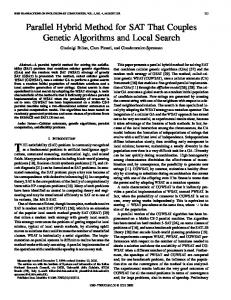
Fig. 1. Box and the Euclidean metrics in

.

Therefore, if and are images on a computer screen, the definition of the Hutchinson metric (1) reduces to

It is sometimes called the box or city-block metric (see Fig. 1). where and

III. HUTCHINSON METRIC REVISITED is a One should recall, for example from [3], that if compact metric space, the Hutchinson metric is defined upon by the set of normalized Borel measures (1) where

and

for all , . The Hutchinson metric gives a notion of the distance between two normalized measures on a compact space and gives rise to the standard weak topology on this space. It is known that the problem of computing this metric is equivalent (by linear programming duality) to a minimum-cost network flow problem, which, in turn, is a special case of the famous Monge–Kantorovich mass transfer problem. The mass transfer problem arises in many areas, such as probability, mathematical economics, IFSs, and digital imaging. is the space where pixels live, In this paper, our space the so-called digitized screen space , where is the screen resolution. is a finite space and therefore every subset of consists of a finite collection of pixels; hence, is a compact metric space. in space can A normalized measure nonnegative real numbers , , and be represented by so that . On the other values , hand, a grayscale image is determined by the where is the intensity of the th pixel. In such a case, it is more than obvious that these values define a measure upon the computer screen that can be normalis defined as ized; this new measure and corresponds to a normalized Borel measure of . By using an appropriate color map, a colored image can be transformed into a normalized Borel measure on . Thus, the association between digitized (color or grey-tone) images and normalized Borel measures on the space of pixels is more than obvious.

, that is, the value of

on the pixel

. Since the summation over the space of pixels is after the simplification finite, the maximum has now taken the place of supremum. We observe that the definition of the Hutchinson distance suggests a standard linear proon the digitized space under the gramming problem for unknown variables . In principle, this constraints problem can be solved using a conventional linear programming algorithm such as the simplex method. The size of the problem, however, is huge: For a screen resolution of pixels, we have a linear programming problem of variables constraints; this makes the problem and hardly feasible under normal computing resources. To overcome this problem, Stark [15] suggested the use of the Box distance as a metric in the space instead of the popular Euclidean distance. Under this simplification, the set of linear constraints becomes (2) . for all , , , Lemma 1: The above-mentioned set of linear restrictions is equivalent to the following set of restrictions for for

and and

.

(3)

Proof: Trivially, any restriction belonging to the first set of restrictions [that is, (2)], also belongs to the second one [that is, (3)]. Conversely, if is a restriction out of set (3), such that and , then

The same trick can be applied also for the other cases ( ), as well. Thus, the sets (2) and (3) are equivalent.

or

DRAKOPOULOS AND NIKOLAOU: EFFICIENT COMPUTATION OF THE HUTCHINSON METRIC

Therefore, the manageable

constraints reduce to a more number of equivalent constraints for for for for

and and and and

1583

TABLE I SIZE OF THE SIMPLEX MATRIX AS A FUNCTION OF THE SCREEN RESOLUTION

(4)

According to J. Stark, a model of neural network based on Tank and Hopfield’s optimization network [16] for solving the above mentioned linear programming problem can be constructed or simulated. As an alternative and feasible proposal, we describe the computation of the Hutchinson metric using the simplex method. then

IV. NEW ALGORITHM One should recall that the simplex method can be employed whenever the variables used in the problem take nonnegative values. Unfortunately, this is not our case. However, we shall prove that a small modification of the objective function can formulate an equivalent form, where all variables are nonnegative. is always true and since either Since or holds, then, without loss of generality, we may assume that . We first need the following important result, for which we have not been able to find a reference in the literature and results in a 2 speed up for the proposed algorithm. exists such that for Lemma 2: An optimal vector whenever . every , be a sufficiently large positive number such Proof: Let as for all , , where is the in an optimal vector; the objective function is then value of transformed as follows:

(5) and we substitute for all , . under The maximum value of the quantity the restrictions (4) is greater than or equal to the maximum value under the restrictions of for for for for

and and and and

From (5), we get

where and are the values of the variables which accomplish the maximum, respectively. Since

and

which implies

Since

and

, then

or

, which implies

If we assume that holds, then we can take are nonnegative variables. for granted that The most usual way of transforming a linear programming problem whose variables are unbounded to an equivalent form where the simplex method can be employed is by introducing and for any unbounded variable . In such two variables a way, we substitute any appearance of with the difference of from , that is and, subsequently, add the , . extra restrictions Because all our variables are unbounded, such a substitution , would, in our case, double the number of variables to is the resolution of the screen. The reader should be where aware that the corresponding simplex tableau is already immense; Table I illustrates this fact better. As one might observe, the size of the simplex matrix is excessively large even for . medium resolutions such that of 500 500 pixels For high resolution, currently used by up-to-date computers, , the matrix/tableau is beyond any effective such as bytes; storage; for such an analysis, we need bytes (we usually need 4 bytes to represent that is, a real number). This amount of memory is unquestionably, more than that available now from any state of the art computer. However, the memory requirements for the storage of the simplex tableau can be dramatically reduced under the simple elements out of the observation that only of the first tableau are nonzero. This can be rows of the explained by the fact that each of the simplex matrix contains only two nonzero entries. Hence, in the

1584

IEEE TRANSACTIONS ON IMAGE PROCESSING, VOL. 13, NO. 12, DECEMBER 2004

case of a medium resolution , the storage requirement total for the simplex tableau is only number of entries which require bytes of memory instead of bytes required for the whole tableau. This means that a 125, 000% cut ) can be acof storage requirements (for the case of complished with the use of sparse matrices techniques. As we shall see later on, the use of such techniques can also be beneficial to the speed of the method, since we do not waste our time on operations which employ zero elements. The following example will highlight the method we employed. Let be the digitized space which corresponds to a screen having the low . Furthermore, we resolution of 2 2 pixels; that is, consider two digitized images and of that resolution. Then, the Hutchinson distance between and is the maximum value of the objective function

TABLE II FIRST SIMPLEX TABLEAU

subject to the constraints

In accordance to what we have already proved, we can assume holds and, therefore, that the hypothesis . Hence, the first simplex we can safely deduce that tableau would be Table II. This tableau can be stored in a conventional computer under the form of an array of linked lists, a structure which can graphically be represented as in Fig. 2. Looking at this figure bottom-up, we first observe four and points to headnodes, each of which corresponds to one one of four linked lists; the nodes of the first list represent the , the nodes of the second represent the nonzero elements of , and so on. The first field inside each nonzero elements of node contains the value of each element, while the second field inside each node contains its position within all elements of the . specific This method of representation of the simplex tableau is primarily responsible for the substantial acceleration of the method (since we are no longer interested in zero entries of the matrix) and for the dramatic reduction in the storage requirements at each stage of the method. V. APPROXIMATION ALGORITHM FOR “LARGE” IMAGES The method, as described in Section IV, was actually employed for the computation of the Hutchinson distance between colored fractals (measures) produced by IFSs. The corresponding algorithm was tested under various screen resolutions and worked efficiently with satisfactory results; however, for 256 pixels, the time screen resolutions that exceeded 256

Fig. 2. Sparse representation of the 

from Table II.

requirements were too great for the various machines we had at our disposal. One should note, however, that the value of the objective function achieved in every iteration of the simplex method is always increasing or, in the worst case, nondecreasing; thus, we always obtain a better and better approximation for the Hutchinson distance at every iteration. These values are actually some lower bounds for the Hutchinson distance until the exact value is eventually achieved and the method terminates. However, no one has ever found an analytic formula which specifies an upper and a lower bound for the optimal value of the objective function; this is justified by the fact that the simplex method is bound to terminate. In such a case, the optimal value is obtained. To overcome the problems induced by the large computation time of the Hutchinson distance between two higher resolution images, the following approximation algorithm is proposed. and let be a Let the screen be of resolution divisor of , that is . Then, as the Fig. 3 squares any suggests, our screen can be partitioned into pixels, where . If and of which will contain are two digitized images with resolution , then we can

DRAKOPOULOS AND NIKOLAOU: EFFICIENT COMPUTATION OF THE HUTCHINSON METRIC

1585

TABLE III IFS CODE FOR A DENDRITE

TABLE IV IFS CODE FOR A FERN LEAF

Fig. 3.

Partition of our screen into M

2 M squares.

easily calculate the pixel values of two corresponding images and whose resolution is only . In this case

TABLE V IFS CODE FOR THE SIERPIN´ SKI TRIANGLE

and

for all , . Now that the two images— and —have a resolution of , we can safely compute their Hutchinson distance only within reasonable time limits. This distance gives an approximation for the actual Hutchinson distance of and . The actual value of the Hutchinson distance is obtained when. The smaller the value of , the more quickly the ever algorithm is executed; however, the bigger the , the better the approximation for the Hutchinson distance. The accuracy of an analytical measurement is how close a result comes to the true value. Therefore a compromise between speed and accuracy is necessary; if one does not wish to wait for hours until the exact value is obtained, one will have to be content with approximations of the distance.

TABLE VI IFS CODE FOR A SPIRAL

TABLE VII BOX, EUCLIDEAN, AND HUTCHINSON ( = 4) DISTANCE BETWEEN THE FRACTAL OBJECTS AND THE COMPUTATION TIME IN HOUR:MINUTE:SECOND FORMAT OF THE THIRD DISTANCE

VI. APPLICATION ON FRACTAL SETS AND REAL-WORLD IMAGES The easiest method for rendering a fractal image is with the aid of the random iteration algorithm (RIA). In the RIA, from its we calculate at each stage just one new point by with a randomly chosen predecessor from . Given a large number of iterations—say 100,000—it works. We refer the interested reader to [3] or [10]. The IFS codes for the under-examination fractal objects are presented in Tables III–VI. The corresponding fractal images are illustrated in Fig. 6. The resolution of the fractal objects considered is 256 256 and the number of iterations is 100, 000. Table VII shows the results of our algorithm with regard to the Box, the Euclidean and the Hutchinson distance between

the fractal attractors, as well as the CPU (computation) time in hours:minutes:seconds format of the third distance. The computation time of the Box and the Euclidean distance is practically zero. Looking at the values of all the distances, we observe that

1586

IEEE TRANSACTIONS ON IMAGE PROCESSING, VOL. 13, NO. 12, DECEMBER 2004

Fig. 5. Original images of (left) Lena and (right) Barbara used in our experiments 256 256 8 bpp.

2

2

2

2

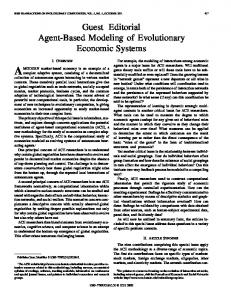
Fig. 4. Dendrite, a fern leaf, a spiral, the Sierpin´ ski triangle, and a transformed version of it.

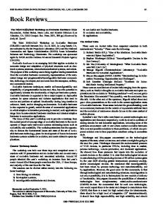
the most dissimilar objects are the {leaf, triangle} pair, whereas the most similar ones are the {dendrite, spiral} pair (Fig. 4). All the pairs have almost the same computation time. Therefore, the similarity between the images does not affect the speed of the algorithm. The strength of the Hutchinson metric versus the other metrics for comparing objects can be seen in the comparison of the pairs {dendrite, triangle} and {triangle, spiral}. Initially, looking at their Box and Euclidean distances, one can be easily led into misperceiving that the latter pair contains the more similar objects; however, their Hutchinson distance is smaller for the first pair, which recommends a new approach to evaluate in a better way the correct discrepancy between the two objects (compare the results with those in [8]). Compare also the distances between the Sierpin´ ski triangle and the transformed version of it that arises if we slightly alter its IFS code; taking, for example , then , , and . Although and suggest, after looking at suggests Table VII, that the two triangles are very different, that they are very close to each other, which is the case. Another thing that must be mentioned is that the Hutchinson distance depends on the random distribution of the points which form the attractor. This is also the case for the other two metrics that depend on the density of the points which form the invariant measure of the distribution. So, it is possible that two consecutive runnings of the RIA to give us different values for the , and (but consistent concerning the order). Most digital-image-compression methods required in realworld applications are lossy compression methods, i.e., the decompressed images must be visually similar, not necessarilly identical, to the original images. So, there is always a tradeoff between the compression ratio and the reconstruction error. We now present typical results from the application of our algorithm to real imagery, aiming to demonstrate its applicability to the demanding problems inherent in the image compression area and its performance. The original images used as our reference point in the experiments presented here are the 256 256 8 bpp Lena and Barbara images shown in Fig. 5. We examine for each original image how close it is to a filtered or compressed replica of it. In other words, we seek to measure the difference (i.e.,

Fig. 6. The 256 256 8 bpp test images used in our experiments. (a) Lifting scheme, (b) Haar, and (c) Antonini (9,7) filters are used.

the error) between two images by computing the Hutchinson distance between the original image and each of the associated filtered ones. The filter banks used in our simulations include the lifting scheme [Fig. 6(a)], which represents a generic and efficient solution to the perfect inversion problem, the Haar filter as well as the (9,7) pair developed by Antonini et al. [2] (Fig. 6). We have also tested the performance of our scheme to a Joint Photographic Experts Group (JPEG) codec in its Corel 7 implementation, as applied to our test images and to images compressed with the embedded zerotree wavelet (EZW) method [13]. The EZW is known to represent the state-of-the-art in modern image compression [17]. The EZW algorithm is a particularly effective approach to the following two-fold problem: achieving the best image quality for a given compression ratio (bit rate) and encoding the image in such a way that all lower bit-rate encodings are embedded in the beginning of the final bit stream. The symbol stream generated by EZW is entropy (losslessly) encoded to achieve further compression.

DRAKOPOULOS AND NIKOLAOU: EFFICIENT COMPUTATION OF THE HUTCHINSON METRIC

1587

TABLE IX HUTCHINSON DISTANCE d BETWEEN THE REAL-WORLD IMAGES WITH RESPECT TO DIFFERENT VALUES OF THE THRESHOLD 

2

2

Fig. 7. The 256 256 8 bpp test images used in our experiments. (a) EZW Shapiro (9,7) and (b) JPEG compression are used.

TABLE X COMPUTATION TIME t IN HOUR:MINUTE:SECOND FORMAT OF THE HUTCHINSON DISTANCE BETWEEN THE REAL-WORLD IMAGES WITH RESPECT TO DIFFERENT VALUES OF THE THRESHOLD 

2

2

Fig. 8. The 256 256 8 bpp test images used in our experiments. (a) EZW Shapiro (9.7) and (b) JPEG compression are used. TABLE VIII BOX AND EUCLIDEAN DISTANCES BETWEEN THE REAL-WORLD IMAGES

For the image of Lena, we used the filter banks as well as the compression schemes mentioned above. For the image of Barbara, we used only the compression schemes. Fig. 7 shows compressed images of Lena at a ratio of 32:1 using (9,7) discrete wavelet transform (DWT) combined with run-length encoder (RLE) and JPEG coding, respectively. Fig. 8 shows compressed images of Barbara at a ratio of 64:1 using (9,7) DWT combined with RLE and JPEG coding, respectively. Table VIII shows the results of our algorithm with regard to the Box and the Euclidean distances between the real-world images. Table IX shows the results of our algorithm with regard to the Hutchinson distance between the real-world images with respect to the threshold value. or Whenever the approximation algorithm is used, i.e. , from Section V, we have . Table X shows

the CPU (computation) time of the third distance in min:sec format with respect to different values of the threshold. The correspondence between the images of Lena and the indices is the original image, lifting scheme, Anfollowing: Haar transform, compression, tonini filter, JPEG compression. The correspondence between the and original images of Barbara and the indices is the following: compression, and JPEG compression. image, Looking at all the pictures of Lena and Barbara, it is not possible to observe at once all of their differences or defects, except for the figures compressed using JPEG. With the help of the Hutchinson distance, it is now possible to look “behind” these images and unveil their imperfections. There are two ways to examine Tables VIII–X: vertically and horizontally. Looking at Tables VIII and IX, from top to bottom, we can see which of the images are closer to the originals. The accuracy of the in approaching the true disapproximation method tance refers to the relative error. We say that a positive is the relative error of the approximation to , number if

1588

IEEE TRANSACTIONS ON IMAGE PROCESSING, VOL. 13, NO. 12, DECEMBER 2004

Therefore, the accuracy of the approximation can be computed from Table IX by taking the maximum of all the individual relative errors. The strength of the Hutchinson metric versus the other metrics for comparing grayscale objects can be seen in the comparand so as and . Initially, ison of the pairs looking at their Box and Euclidean distances, one can be easily led into misperceiving that the latter pairs contain the more similar objects; however, their Hutchinson distance is smaller for the first pair, which recommends a new approach to evaluate, in a better way, the correct discrepancy between the two objects (compare the results with those in [8]). VII. CONCLUSION The current implementation of our algorithms is written in Microsoft Visual Basic 6.0 and is capable of drawing two fractal or open two bitmapped images, as well as to compute their Box, Euclidean, Hausdorff (see [8]), and Hutchinson metrics. The CPU time needed for their computation is also displayed. There exists also a window in which one can see the discrepancy between the two under comparison images (please visit http://cgi.di.uoa.gr/~vasilios/Hausdorff.exe). The whole algorithm was finally tested and rated by computing the distance between attractors produced using the RIA, as well as between grayscale original and transformed real-world images. Time results are given in CPU minutes on a Pentium III PC with a 800-MHz CPU clock running Windows NT 4.0 SP 6. When our algorithm for the computation of the Hutchinson metric is implemented using conventional (serial) machines, then its runtime is close to the one needed for the computation of the Euclidean or the Box distance, which is fairly satisfactory (see Table X). This result holds under the proviso that the approximation algorithm is used. ACKNOWLEDGMENT The authors would like to thank all the referees for their valuable suggestions; they spent a lot of time proofreading, which the authors very much appreciate. REFERENCES [1] I. Aleksander and T. J. Stonham, “A guide to pattern recognition using random-access memories,” Inst. Elect. Eng. J. Comput. Digit. Tech., vol. 2, pp. 29–40, 1979. [2] M. Antonini, M. Barlaud, and P. Mathieu, “Image coding using wavelet transform,” IEEE Trans. Image Processing, vol. 1, pp. 205–220, Feb. 1992. [3] M. F. Barnsley, Fractals Everywhere, 2nd ed. San Diego, CA: Academic, 1993. [4] M. F. Barnsley and S. Demko, “Iterated function systems and the global construction of fractals,” in Proc. Roy. Soc. London, Ser. A, vol. 399, 1985, pp. 243–275. [5] M. F. Barnsley and L. P. Hurd, Fractal Image Compression. Wellesley, MA: AK Peters , 1993. [6] J. Brandt, C. Cabrelli, and U. Molter, “An algorithm for the computation of the Hutchinson distance,” Inform. Process. Lett., vol. 40, pp. 113–117, 1991.

[7] S. Demko, L. Hodges, and B. Naylor, “Construction of fractal objects with iterated function systems,” Comput. Graph., vol. 19, no. 3, pp. 271–278, 1985. [8] V. Drakopoulos and N. Nikolaou, “Efficient computation of the Hausdorff metric between digitised images,” J. Math. Imag. Vis., to be published. [9] Y. Fisher, Ed., Fractal Image Compression: Theory and Application. New York: Springer-Verlag, 1995. [10] S. G. Hoggar, Mathematics for Computer Graphics. Cambridge, U.K.: Cambridge Univ. Press, 1992. [11] J. E. Hutchinson, “Fractals and self similarity,” Indiana Univ. Math. J., vol. 30, pp. 713–747, 1981. [12] T. Kaijser, “Computing the Kantorovich distance for images,” J. Math. Imag. Vis., vol. 9, pp. 173–191, 1998. [13] J. M. Shapiro, “Embedded image coding using zerotrees of wavelet coefficients,” IEEE Trans. Signal Processing, vol. 41, pp. 3445–3462, Dec. 1993. [14] J. Stark, “Iterated function systems as neural networks,” Neural Networks, vol. 4, pp. 679–690, 1991. , “A neural network to compute the Hutchinson metric in fractal [15] image processing,” IEEE Trans. Neural Networks, vol. 2, pp. 156–158, Feb. 1991. [16] D. W. Tank and J. J. Hopfield, “Simple neural optimization networks: an a/d converter, signal decision circuit and a linear programming circuit,” IEEE Trans. Circuits Syst. II, vol. 33, pp. 87–95, Jan. 1986. [17] M. Vetterli and J. Kovaˇcevic, Wavelets and Subband Coding. Englewood Cliffs, NJ: Prentice-Hall, 1995.

Vassileios Drakopoulos was born in Athens, Greece, on July 27, 1968. He received the B.S. degree in mathematics, the M.S. degree in informatics and operations research, and the Ph.D. degree in theoretical informatics from the National and Kapodistrian University of Athens in 1990, 1992, and 1999, respectively. He is a School Adviser and a Research Fellow in the Department of Informatics and Telecommunications, University of Athens. He has taught a number of courses at the University of Athens, as well as in secondary education. During his graduate studies, he began studying with dynamic systems and fractals. After completing the Ph.D. degree, he received a Postdoctoral Scholarship from the (Greek) State Scholarships Foundation (I.K.Y) and has worked on parallel visualization methods. His research interests include fractal and computational geometry, computer graphics, dynamic systems, computational complex analysis, and image compression.

Nikolaos P. Nikolaou received the B.Sc. degree in mathematics from the University of Athens, Athens, Greece, and the M.Sc. degree in foundations of advanced information technology (with distinction) from the Department of Computing, Imperial College, University of London, London, U.K. He is currently pursuing the Ph.D. degree at the Department of Industrial Management and Technology, University of Piraeus, Greece. After receiving the B.Sc. degree, he studied computer science and operations research at the Department of Informatics, University of Athens, as well as information technology at the Department of Computing, Imperial College, University of London. He is the coauthor of five papers in peer-reviewed journals and has presented portions of his work in a series of international conferences. His current research interest includes knowledge representation, engineering modeling, and internet application technologies.