Efficient encoding of low-density parity-check codes - CiteSeerX
Recommend Documents
Thomas J. Richardson and Rüdiger L. Urbanke. AbstractâLow-density ..... term is typically very small so that the encoding complexity stays manageable up to ...
encoding of linear binary cyclic codes is used which improves the encoding ... without involving computers after generating an encoding table for the code.
Mail Code 136-93. Pasadena CA 91125. Email: flihao,[email protected]. Abstract. We present a new class of MDS array codes of size n n (n a prime ...
Jul 8, 2011 - A.A. Andrade and R. Palazzo Jr. [1] discussed the cyclic, BCH, alternant,. Goppa and Srivastava codes over finite rings, which are in fact ...
Nov 23, 2006 - MATLAB1 is nowadays one of the most practical software used for numerical ... This will also help you reuse your functions and create ... Email: reza.sameni @ gmail.com ..... //www.mathworks.com/access/helpdesk/help/pdf ...
Yeow Meng Chee, Chrisnata Johan, Han Mao Kiah, San Ling, Tuan Thanh Nguyen, and ... hence can store one bit per cell. ... with the ability to store log2 q bits per cell. ..... [1] J.-D. Lee, S.-H. Hur, and J.-D. Choi, âEffects of floating-gate inte
present an e cient method for the lossy encoding of object shapes which are given as 8-connect chain codes [1]. We approximate the object shape by a second ...
email: [email protected]. ABSTRACT. A major problem in object oriented video coding is the e cient encoding of the shape information of arbitrarily.
the Web to assess whether CODES was convenient and easy to use, whether decision entry and viewing and printing output were simple, and .... learners are presented with opportunities to build on prior knowledge and understanding ...
Oct 13, 2014 - bits to store a prefix code with average codeword length within an ... An instantaneous code assigns a binary code ci to each symbol ai so that.
Nov 3, 2011 - code: i) a trivalent graph ii) an embedding of the graph on a surface so .... s2 s1 e0 e1 e2 e3 sl. 0 s2 s1. FIG. 8. Splitting the shared syndromes.
IT] 27 Jan 2012. An Efficient Construction of Self-Dual Codes. Yoonjin Leeâ. Department of Mathematics. Ewha Womans University. 11-1 Daehyun-Dong, ...
Email: {wuebben,rinas,boehnke,kuehn,kammeyer}@ant.uni-bremen.de. Abstractâ Layered ... This new algorithm is compared to V-BLAST by simulation results ...
protection, enabling systems to reconstruct lost data when components fail. Erasure codes can however impose sig- nificant performance overhead in two core ...
adopted as the recording code for the Compact Disc (CD). EFMPlus [3], used in ..... The Power Spectral Density (PSD), H ( f ), and other rel' evant characteristics ...
The performance of modern Java Virtual Machines. (VMs) is ... wcli â SUN HotSpot Client 1.3.0-C for Win32, ... Java vs Native Method Invocations â times in [ns].
space-time codes (STC) have been introduced to use space as a second dimension of coding. Layered space-time (LST) codes are a special kind of STC.
broadcast; 3) a post-delivery file repair phase where individual users are served to complete the recovery of their file. In this work we specifically focus on phase ...
accumulate unit (MAC) when implemented on reconfigurable fabric, is inferior to a well designed ASIC arithmetic logic unit (ALU) in terms of both speed and ...
Page 1. Page 2. Page 3. Page 4. Page 5.
accumulate unit (MAC) when implemented on reconfigurable fabric, is inferior to a well designed ASIC arithmetic logic unit (ALU) in terms of both speed and ...
Hamming codes, burst correction, RAID architectures, disk arrays. .... RAID-4 type of architectures, a number of disks carry data ... recover our original data.
Hamming codes maximize the possible rate given these design constraints. ...
code is presented based on the relation between Hamming codes over GF(q ...
ensembles displays distortion saturation for the lossy binary symmetric source coding problem with the belief propagation guided decimation (BPGD) algorithm, ...
Efficient encoding of low-density parity-check codes - CiteSeerX
638. IEEE TRANSACTIONS ON INFORMATION THEORY, VOL. 47, NO. 2, FEBRUARY 2001. Efficient Encoding of Low-Density Parity-Check. Codes. Thomas J.
638
IEEE TRANSACTIONS ON INFORMATION THEORY, VOL. 47, NO. 2, FEBRUARY 2001
Efficient Encoding of Low-Density Parity-Check Codes Thomas J. Richardson and Rüdiger L. Urbanke
Abstract—Low-density parity-check (LDPC) codes can be considered serious competitors to turbo codes in terms of performance and complexity and they are based on a similar philosophy: constrained random code ensembles and iterative decoding algorithms. In this paper, we consider the encoding problem for LDPC codes. More generally, we consider the encoding problem for codes specified by sparse parity-check matrices. We show how to exploit the sparseness of the parity-check matrix to obtain efficient encoders. For the (3 6)-regular LDPC code, for example, the complexity of encoding is essentially quadratic in the block length. However, we show that the associated coefficient can be made quite small, so that 100 000 is still quite practical. encoding codes even of length More importantly, we will show that “optimized” codes actually admit linear time encoding. Index Terms—Binary erasure channel, decoding, encoding, parity check, random graphs, sparse matrices, turbo codes.
I. INTRODUCTION OW-DENSITY parity-check (LDPC) codes were originally invented and investigated by Gallager [1]. The crucial innovation was Gallager’s introduction of iterative decoding algorithms (or message-passing decoders) which he showed to be capable of achieving a significant fraction of channel capacity at low complexity. Except for the papers by Zyablov and Pinsker [2], Margulis [3], and Tanner [4] the field then lay dormant for the next 30 years. Interest in LDPC codes was rekindled in the wake of the discovery of turbo codes and LDPC codes were independently rediscovered by both MacKay and Neal [5] and Wiberg [6].1 The past few years have brought many new developments in this area. First, in several papers Luby, Mitzenmacher, Shokrollahi, Spielman, and Stemann introduced new tools for the investigation of message-passing decoders for the binary-erasure channel (BEC) and the binary-symmetric channel (BSC) (under hard-decision message-passing decoding) [9], [10], and they extended Gallager’s definition of LDPC codes to include irregular codes (see also [5]). The same authors also exhibited sequences of codes which, asymptotically in the block length, provably achieve
L
Manuscript received December 15,1999; revised October 10, 2000. This work was performed while both authors were at Bell Labs, Lucent Technologies, Murray Hill, NJ 07974 USA. T. J. Richardson was with Bell Labs, Lucent Technologies, Murray Hill, NJ 07974 USA. He is now with Flarion Technologies, Bedminster, NJ 07921 USA (e-mail: [email protected]). R. L. Urbanke was with Bell Labs, Lucent Technologies, Murray Hill, NJ 07974 USA. He is now with EPFL, LTHC-DSC, CH-1015 Lausanne, Switzerland (e-mail: [email protected]). Communicated by D. A. Spielman, Guest Editor. Publisher Item Identifier S 0018-9448(01)00739-8. 1Similar
concepts have also appeared in the physics literature [7], [8].
capacity on a BEC. It was then shown in [11] that similar analytic tools can be used to study the asymptotic behavior of a very broad class of message-passing algorithms for a wide class of channels and it was demonstrated in [12] that LDPC codes can come extremely close to capacity on many channels. In many ways, LDPC codes can be considered serious competitors to turbo codes. In particular, LDPC codes exhibit an asymptotically better performance than turbo codes and they admit a wide range of tradeoffs between performance and decoding complexity. One major criticism concerning LDPC codes has been their apparent high encoding complexity. Whereas turbo codes can be encoded in linear time, a straightforward encoder implementation for an LDPC code has complexity quadratic in the block length. Several authors have addressed this issue. 1) It was suggested in [13] and [9] to use cascaded rather than bipartite graphs. By choosing the number of stages and the relative size of each stage carefully one can construct codes which are encodable and decodable in linear time. One drawback of this approach lies in the fact that each stage (which acts like a subcode) has a length which is, in general, considerably smaller than the length of the overall code. This results, in general, in a performance loss compared to a standard LDPC code with the same overall length. 2) In [14] it was suggested to force the parity-check matrix to have (almost) lower triangular form, i.e., the ensemble of codesisrestrictednotonlybythedegreeconstraintsbutalso by the constraint that the parity-check matrix have lower triangular shape. This restriction guarantees a linear time encoding complexity but, in general, it also results in some loss of performance. It is the aim of this paperto showthat,even without cascade constructions or restrictions on the shape of the parity-check matrix, the encoding complexity is quite manageable in most cases and -regprovably linear in many cases. More precisely, for a ular code of length the encoding complexity seems indeed to but the actual number of operations required is be of order , and, because of the extremely no more than small constant factor, even large block lengths admit practically feasible encoders. We will also show that “optimized” irregular codes have a linear encoding complexity and that the required . amount of preprocessing is of order at most The proof of these facts is achieved in several stages. We first show in Section II that the encoding complexity is upper, where , the gap, measures in some way to bounded by be made precise shortly, the “distance” of the given parity-check matrix to a lower triangular matrix. In Section III, we then discuss several greedy algorithms to triangulate matrices and we
RICHARDSON AND URBANKE: EFFICIENT ENCODING OF LOW-DENSITY PARITY-CHECK CODES
639
show that for these algorithms, when applied to elements of a given ensemble, the gap concentrates around its expected value -regwith high probability. As mentioned above, for the ular code the best greedy algorithm which we discuss results in . Finally, in Section IV, we prove that an expected gap of for all known “optimized” codes the expected gap is actually of , resulting in the promised linear encoding order less than complexity. In practice, the gap is usually a small constant. The bound can be improved but it would require a significantly more complex presentation. We finish this section with a brief review of some basic notation and properties concerning LDPC codes. For a more thorough discussion we refer the reader to [1], [11], [12]. LDPC codes are linear codes. Hence, they can be expressed as the null space of a parity-check matrix , i.e., is a codeword if and only if The modifier “low-density” applies to ; the matrix should , where is be sparse. For example, if has dimension even, then we might require to have three ’s per column and six ’s per row. Conditioned on these constraints, we choose at random as discussed in more detail below. We refer to the as-regular LDPC code. The sparseness of sociated code as a enables efficient (suboptimal) decoding, while the randomness ensures (in the probabilistic sense) a good code [1]. -Regular Code of Example 1. [Parity-Check Matrix of Length ]: The following matrix will serve as an example.
(1)
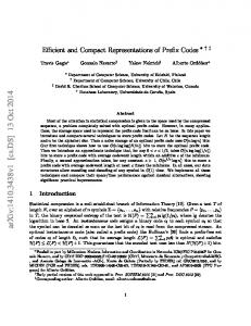
In the theory of LDPC codes it is customary and useful not to focus on particular codes but to consider ensembles of codes. These ensembles are usually defined in terms of ensembles of bipartite graphs [13], [15]. For example, the bipartite graph which represents the code defined in Example 1 is shown in Fig. 1. The left set of nodes represents the variables whereas the right set of nodes represents the constraints. An ensemble of bipartite graphs is defined in terms of a pair of degree distriis simply a butions. A degree distribution polynomial with nonnegative real coefficients satisfying . Typically, denotes the fraction of edges in a graph which are incident to a node (variable or constraint node as the case may be) of degree . In the sequel, we will use the shorthand to denote
This quantity gives the inverse of the average node degree. Asis the rate sociated to a degree distribution pair defined as (2)
Fig. 1. Graphical representation of a (3; 6)-regular LDPC code of length 12. The left nodes represent the variable nodes whereas the right nodes represent the check nodes.
For example, for the degree distribution pair , which -regular LDPC code, the rate is . corresponds to the of degree distributions and a natural Given a pair number , we define an ensemble of bipartite graphs in the following way. All graphs in the ensemble will have left nodes which are associated to and right nodes which are associated to . More precisely, assume that
and We can convert these degree distributions into node perspective by defining and Each graph in has left nodes of degree and right nodes of degree . The order of these nodes is arbitrary but fixed. Here, to simplify notation, we assume that and are chosen in such a way that all these quantities are integer. A node of degree has sockets from which the edges emanate and these sockets are ordered. Thus, in total there are
ordered sockets on the left as well as on the right. Let be a . We can associate a graph permutation on to such a permutation by connecting the th socket on the left th socket on the right. Letting run over the set of to the permutations on generates a set of graphs. Endowed with the . uniform probability distribution this is the ensemble Therefore, if in the future we choose a graph at random from the then the underlying probability distribution ensemble is the uniform one.
640
IEEE TRANSACTIONS ON INFORMATION THEORY, VOL. 47, NO. 2, FEBRUARY 2001
It remains to associate a code to every element of . We will do so by associating a parity-check matrix to each graph. At first glance, it seems natural to define the parityas check matrix associated to a given element in -matrix which has a nonzero entry at row and that column if and only if (iff) the th right node is connected to the th left node. Unfortunately, the possible presence of multiple edges between pairs of nodes requires a more careful definition. Since the encoding is done over the field GF , we as the matrix which define the parity-check matrix has a nonzero entry at row and column iff the th right node is connected to the th left node an odd number of times. As we will see, the encoding is accomplished in two steps, a preprocessing step, which is an offline calculation performed once only for the given code, and the actual encoding step which is the only data-dependent part. For the preprocessing step it is more natural to work with matrices which contain the multiplicities of edges and, therefore, we define the extended as that matrix which has an entry at parity-check matrix row and column iff the th right node is connected to the th left node by edges. Clearly, is equal to modulo . In the sequel, we will also refer to these two matrices as the adjacency matrix and the extended adjacency matrix of the bipartite graph. Since for every graph there is an associated code, we will use these two terms interchangeably so we will, . e.g., refer to codes as elements of Most often, LDPC codes are used in conjunction with message- passing decoders. Recall that there is a received message associated to each variable node which is the result of passing the corresponding bit of the codeword through the given channel. The decoding algorithm proceeds in rounds. At each round, a message is sent from each variable node to each neighboring check node, indicating some estimate of the associated bit’s value. In turn, each check node collects its incoming messages and, based on this information, sends messages back to the incident variable nodes. Care must be taken to send out only extrinsic information, i.e., the outgoing message along a given edge must not depend on the incoming message along the same edge. As we will see, the preprocessing step for the encoding is closely related to the message-passing decoder for the BEC. We will therefore review this particular decoder in more detail. and assume that we Assume we are given a code in use this code to transmit over a BEC with an erasure probability of . Therefore, an expected fraction of the variable nodes will will be known. be erasures and the remaining fraction We first formulate the iterative decoder not as a message-passing decoder but in a language which is more suitable for our current purpose, see [9]. Decoder for the Binary Erasure Channel: 0 . [Intialization] 1 . [Stop or Extend] If there is no known variable node and no check node of degree one then output the (partial) codeword and stop. Otherwise, all known variable nodes and all their adjacent edges are deleted. 2 . [Declare Variables as Known] Any variable node which is connected to a degree one check node is declared to be known. Goto 1.
This decoder can equivalently be formulated as a messagepassing decoder. Messages are from the set with a indicating that the corresponding bit has not been determined yet (along the given edge). We will call a message an erasure message. At a variable node, the outgoing message along an edge is the erasure message if the received message associated to this node is an erasure and if all incoming messages (excluding the incoming message along edge ) are erasure messages, otherwise, the outgoing message is a . At a check node, the outgoing message along an edge is the erasure message if at least one of the incoming messages (excluding the incoming message along edge ) is the erasure message, and a otherwise. If we declare that an originally erased variable node becomes known as soon as it has at least one incoming message which is not an erasure then one can check that at any time the set of known variable nodes is indeed identical under both descriptions. It was shown in [16] that (asymptotically in ) the expected of erasure messages after the th decoding round is fraction given by (3) . Let , called the threshold of the degree where distribution pair, be defined as where (4) is inNote first that the function . It follows by creasing in both its arguments for then for any finite induction that if . If we choose , then the asymptotic expected fraction of erasure messages converges to zero. Consequently, the decoder will be successful with high probability in then, this case. If, on the other hand, we choose with high probability, the decoding process will not succeed. We will see shortly that, correctly interpreted, this decoding procedure constitutes the basis for all preprocessing algorithms that we consider in this paper. Example 2. [(3, 6)-Regular Code]: Let Then . The exact threshold termined in [17] and can be expressed as follows. Let by
where
and
Then
was debe given
RICHARDSON AND URBANKE: EFFICIENT ENCODING OF LOW-DENSITY PARITY-CHECK CODES
Fig. 2. An equivalent parity-check matrix in lower triangular form.
II. EFFICIENT ENCODERS BASED ON APPROXIMATE LOWER TRIANGULATIONS In this section, we shall develop an algorithm for constructing efficient encoders for LDPC codes. The efficiency of the encoder arises from the sparseness of the parity-check and the algorithm can be applied to any (sparse) matrix . Although our example is binary, the algorithm applies generally to matrices whose entries belong to a field . We assume throughout that the rows of are linearly independent. If the rows are linearly dependent, then the algorithm which constructs the encoder will detect the dependency and either or one can eliminate the one can choose a different matrix redundant rows from in the encoding process. parity-check matrix over . Assume we are given an By definition, the associated code consists of the set of -tuples over such that
Fig. 3.
641
The parity-check matrix in approximate lower triangular form.
term is typically very small so that the encoding complexity stays manageable up to very large block lengths. Our proposed encoder is motivated by the above example. Assume that by performing row and column permutations only we can bring the parity-check matrix into the form indicated in Fig. 3. We say that is in approximate lower triangular form. Note that since this transformation was accomplished solely by permutations, the matrix is still sparse. More precisely, assume that we bring the matrix in the form (5) , is , is , where is is , is , and, finally, is . Further, all these matrices are sparse2 and is lower triangular with ones along the diagonal. Multiplying this matrix from the left by (6)
Probably the most straightforward way of constructing an encoder for such a code is the following. By means of Gaussian into an equivalent lower triangular form elimination bring as shown in Fig. 2. Split the vector into a systematic part , , and a parity part , , such that . Construct a systematic encoder as follows: i) Fill with the desired information symbols. ii) Determine the parity-check symbols using back-substitution. More precisely, calculate for
we get (7) where denotes the systematic part, Let and combined denote the parity part, has length , and has length . The defining equation splits naturally into two equations, namely (8) and
What is the complexity of such an encoding scheme? Bringing operations of the matrix into the desired form requires operapreprocessing. The actual encoding then requires tions since, in general, after the preprocessing the matrix will no longer be sparse. More precisely, we expect that we need about XOR operations to accomplish this encoding, where is the rate of the code. Given that the original parity-check matrix is sparse, one . As we might wonder if encoding can be accomplished in will show, typically for codes which allow transmission at rates close to capacity, linear time encoding is indeed possible. And for those codes for which our encoding scheme still leads to quadratic encoding complexity the constant factor in front of the
(9) and assume for the moment that Define is nonsingular. We will discuss the general case shortly. Then from (9) we conclude that
Hence, once the matrix has been precomputed, the determination of can be accomsimply by performing plished in complexity 2More
precisely, each matrix contains at most
O(n) elements.
642
IEEE TRANSACTIONS ON INFORMATION THEORY, VOL. 47, NO. 2, FEBRUARY 2001
TABLE I EFFICIENT COMPUTATION OF p =
0 (0ET
TABLE II EFFICIENT COMPUTATION OF p =
a multiplication with this (generically dense) matrix. This complexity can be further reduced as shown in Table I. Rather and then multiplying than precomputing we can determine by breaking the computation into with several smaller steps, each of which is efficiently computable. , which has complexity To this end, we first determine since is sparse. Next, we multiply the result by . is equivalent to the system Since this can also be accomplished in by back-substitution, since is lower triangular and also sparse. The remaining steps are fairly straightforward. It follows that the overall comis . In a similar manner, plexity of determining , we can accomnoting from (8) that as shown step plish the determination of in complexity by step in Table II. A summary of the proposed encoding procedure is given in Table III. It entails two steps. A preprocessing step and the actual encoding step. In the preprocessing step, we first perform row and column permutations to bring the parity-check matrix into approximate lower triangular form with as small a gap as possible. We will see, in subsequent sections, how this can be accomplished efficiently. We also need to check whether is nonsingular. Rather than premultiplying , this task can be accomplished effiby the matrix ciently by Gaussian elimination. If, after clearing the matrix the resulting matrix is seen to be singular we can simply perform further column permutations to remove this singularity. is not rank deficient, as asThis is always possible when sumed. The actual encoding then entails the steps listed in Tables I and II. We will now demonstrate this procedure by means of our running example. -Regular Code of Example 3. [Parity Check Matrix of Length ]: For this example if we simply reorder the columns such that, according to the original order, we have the ordering 1, 2, 3, 4, 5, 6, 7, 10, 11, 12, 8, 9, then we put the parity-check
0T
(As
A + C )s
+
Bp
)
matrix into an approximate lower triangular form with
We now use Gaussian elimination to clear
(10) . This results in
We see that is singular. This singularity can be removed if we exchange e.g., column 5 with . In terms of the original order column 8 which gives the final column order is then 1, 2, 3, 4, 10, 6, 7, 5, 11, 12, 8, 9, and the resulting equivalent parity-check matrix is
(11)
RICHARDSON AND URBANKE: EFFICIENT ENCODING OF LOW-DENSITY PARITY-CHECK CODES
643
TABLE III SUMMARY OF THE PROPOSED ENCODING PROCEDURE. IT ENTAILS TWO STEPS: A PREPROCESSING STEP AND THE ACTUAL ENCODING STEP
Assume now we choose . To determine we follow the steps listed in Table I. We get
and
In a similar manner, we execute the steps listed in Table II to determine . We get
(13)
and Therefore the codeword is equal to A quick check verifies that
angulation. Hence, for a given parity-check matrix we are interested in finding an approximate lower triangulation with as small a gap as possible. Given that we are interested in large block lengths, there is little hope of finding the optimal row and column permutation which results in the minimum gap. So we will limit ourselves to greedy algorithms. As discussed in the previous section, the following greedy algorithms work on the extended adjacency matrices since these are, except for the ordering of the sockets, in one-to-one correspondence with the underlying graphs. To describe the algorithms we first need to extend some of our previous definitions. Recall that for a given pair of degree distributions we associate to it two important parameters. is the rate of the degree distribution The first parameter pair and is defined in (2). Note that
, as required.
III. APPROXIMATE UPPER TRIANGULATION ALGORITHMS
VIA
GREEDY
We saw in the previous section that the encoding complexity is of order , where is the gap of the approximate tri-
is called the threshold of the The second parameter , degree distribution pair and is defined in (4). If as we have tacitly assumed so far, then we can think of as the degree distribution pair of an ensemble of LDPC codes . Further, as discussed in Section I, in this case it of rate is the threshold of this ensemble was shown in [9] that when transmitting over the BEC assuming a belief propagation may be negative and, hence, the decoder. In general, degree distribution pair does not correspond to an ensemble of LDPC codes. Nevertheless, the definitions are still meaningful.
644
IEEE TRANSACTIONS ON INFORMATION THEORY, VOL. 47, NO. 2, FEBRUARY 2001
Example 4: Let . In this case, we and, using the techniques described in have [17], the threshold can be determined to be
In a similar way, the definition of the ensemble as well as the association of (extended) adjacency matrices to elecarry over to the case . Assume ments of , we create a new ennow that, for a given ensemble semble by simply exchanging the roles of left and right nodes. This new ensemble is equivalent to the ensemble where we have used (13). For the associated (extended) adjacency matrices this simply amounts to transposition. Assume we are given a matrix of dimension with elements in , where is some real-valued parameter with . We will say that a row and a column are connected if the corresponding entry in is nonzero. Furthermore, we will say that a row (column) has degree if its row (column) sum equals . Assume now that we want to bring into approximate lower triangular form. The class of greedy algorithms that we will consider is based on the following simple procedure. Given matrix and a fixed integer , the , permute, if possible, the rows and columns in such a way that the first row has its last nonzero entry at position . If this first step was successful then fix the first row and permute, if possible, the remaining rows and all columns in such a way that the second row has its last nonzero entry at position . In general, assuming that the first steps were successful, permute at the th step, if possible, the last rows and all columns in such a way that the th row has . If this procedure its last nonzero entry at position does not terminate before the th step then we accomplished an approximate lower triangulation of the matrix . We will say that is in approximate lower triangular form with row gap and column gap , as shown in Fig. 4. A. Greedy Algorithm A We will now give a precise description of the greedy algorithm A. The core of the algorithm is the diagonal extension step. Diagonal Extension Step: Assume we are given a matrix and a subset of the columns which are classified as known. In all cases of interest to us, either none of these known columns are connected to rows of degree one or all of them are. Asdenote the known columns sume the latter case. Let be degree-one rows such that is connected and let to .3 Reorder, if necessary, the rows and columns of such form the leading rows of and such that that form the leading columns of as shown in Fig. 5, where denotes the submatrix of which results from deleting and . the rows and columns indexed by submatrix of Note that after this reordering the top-left has diagonal form and that the top rows of have only this one nonzero entry. 3
may not be determined uniquely.
Fig. 4. Approximate lower triangulation of the matrix A with row gap (1 r )l k and column gap l k achieved by a greedy algorithm.
0
0
0
Fig. 5. Given the matrix A let ; . . . ; denote those columns which are connected to rows of degree one and let ; . . . ; be degree-one rows such that is connected to . Reorder the rows and columns in such a way that ; ...; form the first k rows and such that ; . . . ; form the first k columns. Note that the top-left k k submatrix has diagonal form and that the first k rows have only this one nonzero entry.
2
By a diagonal extension step we will mean the following. As input, we are given the matrix and a set of known columns. The algorithm performs some row and column permutations and specifies a residual matrix . More precisely, if none of the known columns are connected to rows of degree one then perform a column permutation so that all the known columns form the leading columns of the matrix . Furthermore, delete these known columns from the original matrix and declare the resulting matrix to be . If, on the other hand, all known columns are connected to rows of degree one then perform a row and column permutation to bring into the form depicted in Fig. 5. Furthermore, delete the known columns and the rows from the original matrix and declare the resulting matrix to be . In terms of this diagonal extension step, greedy algorithm A has a fairly succinct description. Greedy Algorithm A: 0. [Initialization] Given a matrix declare each column indeor, otherwise, pendently to be known with probability . to be an erasure. Let 1. [Stop or Extend] If contains neither a known column nor a row of degree one then output the present matrix. Otherwise, perform a diagonal extension step. 2. [Declare Variables as Known] Any column in which is connected to a degree one row is declared to be known. Goto 1.
RICHARDSON AND URBANKE: EFFICIENT ENCODING OF LOW-DENSITY PARITY-CHECK CODES
645
0
0
Fig. 6. (a) The given matrix A. (b) After the first application of step one, the (1 )l known columns are reordered to form the first (1 )l columns of the matrix A. (c) After the second application of step one, the k new known columns and their associated rows are reordered to form a diagonal of length k . (d) If the procedure does not terminate prematurely then the diagonal is extended to have length l and, therefore, the row gap is equal to (1 r )l and the column gap is equal to (1 )l.
0
To see that greedy algorithm A indeed gives rise to an approximate triangulation assume that we start with the matrix as shown in Fig. 6(a). In the initialization step, an exof all columns are classified as known pected fraction and the rest is classified as erasures. The first time the algorithm known columns are reordered to performs step one these form the leading columns of the matrix as shown in Fig. 6(b). Assuming that the residual matrix has rows of degree one, the columns connected to these degree-one rows are identified in the and let second step. Let these columns be be degree-one rows such that is connected to . During the second application of step one these new known columns and their associated rows are ordered along a diagonal as shown in Fig. 6(c). Furthermore, in each additional iteration this diagonal is extended further. If this procedure does not stop prematurely and, therethen the resulting diagonal has expected length and the column fore, the row gap has expected size as shown in Fig. 6(d). If, on gap has expected size the other hand, the procedure terminates before all columns are exhausted then we get an approximate triangulation by simply reordering the remaining columns to the left. Assuming that the remaining fraction of columns is equal to then the resulting and the resulting expected row gap is equal to . expected column gap is equal to Lemma 1 [Performance of Greedy Algorithm A]: Let be a given degree pair and choose . Pick a graph and let be its extended at random from the ensemble adjacency matrix. Apply greedy algorithm A to the extended adjacency matrix . Then (asymptotically in ) the row gap is and the column gap concentrated around the value . Letting , we is concentrated around the value see that the minimum row gap achievable with greedy algorithm and that the minimum column gap A is equal to . is equal to Proof: Assume we are given a graph and an associated from the ensemble . extended adjacency matrix
0 0
Assume first that so that represents an en. For the same code/graph semble of LDPC codes of rate consider the process of transmission over an erasure channel followed by decoding using the with erasure probability message-passing decoder described in Section I. Compare this procedure to the procedure of the greedy algorithm A. Assume that the bits erased by the channel correspond to exactly those columns which in the initial step are classified as erasures. Under this assumption, one can see that those columns which are declared known in the th round of greedy algorithm A correspond exactly to those variable nodes which are declared known in the th round of the decoding algorithm. Hence, there is a one-to-one correspondence between these two algorithms. then (asymptotAs discussed in Section I, if ically in ) with high probability the decoding process will be successful. Because of the one-to-one correspondence we conclude that in this case (asymptotically in ) greedy algorithm A with will extend the diagonal to (essentially) its full length high probability so that the row and column gaps are as stated in the Lemma. we cannot associate an ensemble In the case that . Nevertheless, of codes to the degree distribution pair recursion (3) still correctly describes the expected progress of greedy algorithm A. It is also easy to see that the concentration around this expected value still occurs. It follows that the same analysis is still valid in this case. 1) Greedy Algorithm AH: By greedy algorithm AH we mean the direct application of greedy algorithm A to the of a given LDPC code. The extended parity-check matrix gap we are interested in is then simply the resulting row gap. Corollary 1 (Performance of Greedy Algorithm AH): Let be a given degree distribution pair with and choose . Pick a code at random from the and let be the associated extended ensemble parity-check matrix. Apply greedy algorithm A to . Then (asymptotically in ) the gap is concentrated around the
646
IEEE TRANSACTIONS ON INFORMATION THEORY, VOL. 47, NO. 2, FEBRUARY 2001
value . Letting , we see that the minimum gap achievable with greedy algorithm A is equal to . -Regular Code and Greedy AlExample 5 [Gap for the gorithm AH]: From Example 2, we know that and that . It follows that the minimum expected gap size for greedy algorithm AH is equal to . Note that greedy algorithm A establishes a link between the error-correcting capability on a BEC using a message-passing decoder and the encoding complexity. In simplified terms: Good codes have low encoding complexity! 2) Greedy Algorithm AHT: Rather than applying greedy algorithm A directly to the extended parity-check matrix of an LDPC code we can apply it to the transpose of the extended parity-check matrix. In this case, the gap we are interested in is equal to the resulting column gap. Corollary 2 (Performance of Greedy Algorithm AHT): Let be a given degree distribution pair with and . Pick a code at random from the ensemble choose and let be the associated extended parity-check ma. Recall that this is equivtrix. Apply greedy algorithm A to alent to applying greedy algorithm A to a randomly chosen ex. tended adjacency matrix from the ensemble Therefore, (asymptotically in ) the gap is concentrated around . Letting , we see that the minthe value imum gap achievable with greedy algorithm AHT is equal to . -Regular Code and Greedy AlExample 6 [Gap for the gorithm AHT]: From Example 4, we know that and that . It follows that the minimum expected gap size for greedy algorithm AHT is equal to
Example 7 (Gap for an “Optimized” Code of Maximal Deand Greedy Algorithm AHT): Let us determine the gree for one of the “optimized” codes listed in threshold [12]. We pick the code with
Lemma 2: Let be a degree distribution pair. Then if and only if for all (14) Furthermore, if (14) holds and
, then (15)
Proof: Clearly, if (14) holds then for any
we
have
By a compactness argument if follows that as defined in . (3) converges to as tends to infinity. Hence, . This means that for any Assume now that we have that . We want to show that and note that for (14) holds. Let , is an increasing function in both its aris increasing in it follows guments. Note that because to converge to zero is that that a necessary condition for , i.e., that at least in the first iteration the erasure probability decreases. We will use contraposition to prove (14). Hence, assume that there exist a strictly positive and an , , such that . Since and since is continuous this implies that there exists a strictly pos, such that . Then itive and an ,
It follows by finite induction that
and, therefore, does not converge to zero as infinity, a contradiction. Finally, for close to one we have
whereas for
tends to
tending to zero we have
This yields the stability conditions stated in (15). and
Quite surprisingly we get ! This means that for we can start the process by declaring only an any fraction of all columns to be known and, with high probability, fraction of all the process will continue until at most an for any columns is left. Therefore, we can achieve a gap of . We will later prove a stronger result, namely, that in this , but we will need case the gap is actually at most of order more sophisticated techniques to prove this stronger result. The above example shows that at least for some degree diswe have . When does this tribution pairs happen? This is answered in the following lemma.
B. Greedy Algorithm B For greedy algorithm A, the elements of the initial set of known columns are chosen independently from each other. We will now show that by allowing dependency in the initial choice, the resulting gap can sometimes be reduced. Of course, this dependency makes the analysis more difficult. In order to describe and analyze greedy algorithm B we need to introduce some more notation. We call a polynomial
with real nonnegative coefficients in the range a weight distribution, and we denote the set of all such weight distribube a map which maps a pair tions by . Let
RICHARDSON AND URBANKE: EFFICIENT ENCODING OF LOW-DENSITY PARITY-CHECK CODES
consisting of a degree distribution into a new degree distribution
and a weight distribution . This map is defined as
We are now ready to state greedy algorithm B. Greedy Algorithm B: 0. [Initialization] We are given a matrix and a weight dis. For each row in perform the following: if tribution the row has weight then select this row with probability . For each selected row of weight declare a random subset of its connected columns to be known. All of size remaining columns which have not been classified as known . are classified as erasures. Let 1. [Stop or Extend] If neither contains a known column nor a row of degree one then output the present matrix. Otherwise, perform a diagonal extension step. 2. [Declare Variables as Known] Any column in which is connected to a degree one row is declared to be known. Goto 1 Clearly, greedy algorithm B differs from greedy algorithm A only in the choice of the initial set of columns. be a Lemma 3 (Analysis of Greedy Algorithm B): Let be a weight distribution given degree distribution pair. Let . Define . such that and let Pick a graph at random from the ensemble be its extended adjacency matrix. Apply greedy algorithm B to the extended adjacency matrix . Then (asymptotically in ) the row gap is concentrated around the value
and the column gap is concentrated around the value
Proof: The elements of the initial set of known columns are clearly dependent (since groups of those columns are connected to the same row) and therefore we cannot apply our previous methods directly. But as we will show now there is a one-to-one correspondence between applying greedy algorithm with a weight distribution B to the ensemble and applying greedy algorithm A to the transformed ensemble . and a weight disAssume we are given the ensemble . Assume further that we are given a fixed set of tribution and that the fraction of selected right nodes (rows) selected right nodes of degree is equal to . Given a graph transform it in the following way: replace each from selected right node of degree by right nodes of degree . One can check that this transformation leaves the left degree distribution unchanged and that it transforms the right degree dis-
647
tribution to . Therefore, the new graph is an element . Further, one can check that this of the ensemble map is reversible and, therefore, one-to-one. A closer look reveals now that applying greedy algorithm B to an extended adjacency matrix picked randomly from the ensemble is equivalent to applying greedy algorithm A with to the transformed extended adjacency matrix, i.e., the resulting residual graphs (which could be empty) will be the same. Now, it follows that the greedy algorithm B will since we get started and since by assumption know from the analysis of greedy algorithm A that with high probability the diagonalization process will continue until the diagonal has been extended to (essentially) its full length. In this case, the resulting column gap is equal to the size of the set which was initially classified as known. To determine the size of this set we first determine the probability that a randomly chosen edge is one of those edges which connect a selected right node declared known neighbors. A quick calculato one of its . tion shows that this probability is equal to Therefore, the probability that a given left node of degree is . connected to at least one of these edges is equal to From this the stated row and column gaps follow easily. 1) Greedy Algorithm BH: Following our previous notation, by greedy algorithm BH we mean the direct application of greedy algorithm B to the extended parity-check matrix of a given LDPC code. The gap we are interested in is then simply the resulting row gap. Corollary 3 (Performance of Greedy Algorithm BH): Let be a given degree distribution pair with . Let be a weight distribution such that . Define
Pick a code at random from the ensemble and let be its extended parity-check matrix. Apply greedy algorithm B to the extended parity-check matrix . Then (asymptotically in ) the gap is concentrated around the value
Let
Then we see that the minimum gap achievable with greedy algorithm BH is equal to
Example 8 [Gap for the -Regular Code and Greedy Aland and since gorithm BH]: We have has only one nonzero term it follows that we can param-
648
eterize
IEEE TRANSACTIONS ON INFORMATION THEORY, VOL. 47, NO. 2, FEBRUARY 2001
as
. Therefore, we have and since , it follows that we need to find the smallest value of , call it , such that . From Lemma (14) we see that a necessary and sufficient condition is given by
Example 9 [Gap for the -Regular Code and Greedy Aland and since gorithm BHT]: We have has only one nonzero term we can parameterize as . Therefore, we have and since it follows that we need to find the smallest . value of , call it , such that From Lemma 2 (14) we see that a necessary and sufficient condition is given by
Equivalently, we get
which simplifies to Differentiating shows that the right-hand side takes on its minimum at the unique positive root of the polynomial . If we call this root , with , then we conclude that
We then get equal to
By differentiating minimum at by
we find that it takes its . Thus, the critical value of is given
and, therefore, the gap is We then get
Note that in this case the gap is larger than the corresponding gap for greedy algorithm AH. 2) Greedy Algorithm BHT: Again as for greedy algorithm A, rather than applying greedy algorithm B directly to the exof an LDPC code we can apply tended parity-check matrix it to the transpose of the extended parity-check matrix. In this case, the gap we are interested in is equal to the resulting column gap. Corollary 4 (Performance of Greedy Algorithm BHT): Let be a given degree distribution pair with . be a weight distribution such that Let Define . Pick a code at random from the enand let be its extended parity-check matrix. semble . Recall that this is equivalent Apply greedy algorithm B to to applying greedy algorithm B to a randomly chosen extended . Thereadjacency matrix from the ensemble fore, (asymptotically in ) the gap is concentrated around the value
Let
Then we see that the minimum gap achievable with greedy algorithm BHT is equal to
. This corresponds to a gap of
This is significantly better than the corresponding gap for greedy algorithm AHT. C. Greedy Algorithm C be the given degree distribution pair. Recall that Let for greedy algorithm B we chose the weight distribution in such a way that . Hence, with high probability, the greedy algorithm will extend the diagonal to (essentially) its full length. Alternatively, we can try to achieve an approximate triangulation in several smaller steps. More precisely, assume in such a way that that we pick the weight distribution . Then with high probability the greedy algorithm will not complete the triangulation process. Note that, conditioned on the size and on the degree distribution pair of the resulting residual graph, the edges of this residual graph are still random, i.e., if the residual graph has length and a then we can think of it as an degree distribution pair . This is probably easiest seen by checking element of that if the destination of two edges which are contained in the residual graph are interchanged in the original graph and if the greedy algorithm B is applied to this new graph then the new residual graph will be equal to the old residual graph except for this interchange. Therefore, if we achieve a triangulation by applying several small steps, then we can still use the previous tools to analyze the expected gap. There are obviously many degrees of freedom in the choice of step sizes and the choice of weight distribution. In our present discussion, we will focus on the limiting case of infinitesimal small step sizes and a constant weight distribution. Therefore, and assume that we are given a fixed weight distribution , be a small scaling parameter for the weights such let ,
RICHARDSON AND URBANKE: EFFICIENT ENCODING OF LOW-DENSITY PARITY-CHECK CODES
that . Assume that we apply greedy algorithm B to a randomly chosen element of the ensemble where . We claim that the expected degree , is given by distribution pair of the residual graph, call it
649
iff at least one of its incoming messages is not an erasure—otherwise, it stays and retains its degree. Using (16) we see that a node of degree has a probability of
of being expurgated. Since in the original graph the number of it follows that in the left degree nodes is proportional to residual graph the number of left degree nodes is proportional to
To see this, first recall from the analysis of greedy algorithm B that the degree distribution pair of the equivalent trans. Since by assumption formed graph is equal to , the recursion given in (3) (with ) , will have a fixed point, i.e., there exists a real number , such that
From an edge perspective the degree fraction of the residual graph is, therefore, proportional to
After normalization we find that the left degree distribution of the residual graph, call it , is given by in
To determine this fixed point note that if we expand the above around we obtain
We next determine the right degree distribution of the residual graph. Recall that the equivalent transformed graph has a right . We are only interested in nodes degree distribution of of degree at least two. Hence we have Therefore, letting
denote
, the fixed-point equation
is From a node perspective these fractions are proportional to
It follows that
In the language of message-passing algorithms, is the expected fraction of erasure messages passed from left to right at the time the algorithm stops. The fraction of erasure messages which are passed at that time from right to left is then
(16) We start by determining the residual degree distribution of left nodes. Note that a left node will not appear in the residual graph
Define the erasure degree of a right node to be equal to the number of incoming edges which carry erasure messages. To first order in , a node of erasure degree can stem either from a node of regular degree all of whose incoming messages are erasures or it can stem from a node of regular degree which has one nonerasure message. Hence, at the fixed point the fraction of right nodes with an erasure degree of is proportional to
Converting back to an edge perspective we see that these fractions are proportional to
650
Summing the above over
IEEE TRANSACTIONS ON INFORMATION THEORY, VOL. 47, NO. 2, FEBRUARY 2001
we obtain
Noting that and normalizing we see that the residual right degree distribution, call it , is given by
in which case we are interested in the resulting column gap or we can apply it to the transpose of the extended paritycheck matrix in which case we are interested in the column gap. We call these algorithms CH and CHT, respectively. -Regular Code and Greedy AlExample 10 [Gap for and let where gorithm CHT]: We choose is some very small quantity. Solving the system of differential . We equations reveals that the resulting gap is equal to see that this is the smallest expected gap for all the presented algorithms. D. A Practical Greedy Algorithm
We are ultimately interested in the resulting row and column gaps. Since one can easily be determined from the other we will only write down an expression for the row gap. If we take the expression for the row gap, call it from greedy algorithm B, and keep only the terms which are linear in then we see that the row gap increased according to
The length of the code itself evolves as
In practice, one implements a serial version of greedy algorithm CHT. At each stage, if the residual graph has a degree-one variable node then diagonal extension is applied. If no such degree-one variable node exists then one selects a variable node of lowest possible degree, say, from the residual graph, and (assuming no multiple edges) of its neighbors to declares be known. The residual graph now has at least one degree-one node and diagonal extension is applied. There are many practical concerns. For example, variable nodes which are used in the diagonal extension step correspond to nonsystematic variables. Typically, degree-two nodes have the highest bit-error rates. Thus, it is preferable to use as many low-degree variables in the diagonalization step as possible, e.g., if the subgraph induced by only the degree-two variables has no loops then all degree-two variables can be made nonsystematic using the above algorithm. IV. CODES WITH LINEAR ENCODING COMPLEXITY
Collecting all results we see that as a function of the independent variable all quantities evolve according to the system of differential equations
We saw in the preceding section that degree distributions giving rise to codes that allow transmission close to capacity will have gaps that are smaller than an arbitrarily small linear fraction of the length of the code. To prove that these codes have linear encoding complexity more work is needed, namely, with high one has to show that the gap satisfies probability for large enough . More precisely, we will prove the following. Theorem 1 (Codes with Linear Encoding Complexity): Let be a degree distribution pair satisfying , , and satisfying the strict with minimum right degree . Let be chosen at random from inequality . Then is encodable in linear time with the ensemble for some positive constants and probability at least , where .
with the value of the initial quantities equal to , , , and , respectively. As before, we can apply greedy algorithm C directly to the extended parity-check matrix chosen randomly from an ensemble
Discussion: We note that all optimized degree distribution pairs listed in [12] fulfill the conditions of Theorem 1. Furthermore, in experiments when applying the practical greedy algorithm to graphs based on these degree distribution pairs, the resulting gap is typically in the range of one to three! This is true even for very large lengths like one million. By correctly choosing the first degree-two variable, the gap can nearly always be lowered to one. The primary reason for these very small gaps is the large number of degree-two variable nodes in these degree distributions. The number of degree-two variable nodes is suf-
RICHARDSON AND URBANKE: EFFICIENT ENCODING OF LOW-DENSITY PARITY-CHECK CODES
ficiently large so that, with very high probability, the subgraph induced by these nodes has a large (linear size) connected component. Once a single check node belonging to this component is declared known then the remainder of the component will diagonalize in the next diagonal extension step. The diagonalization process then typically completes without further increasing the gap. Proof: In order to show that under the stated conditions are linear time encodelements of the ensembles able (with high probability) it suffices to show that their can be brought into approximate lower corresponding (with high triangular form with a gap of no more than probability). Note that we are working on the transpose of the parity-check matrix. Although one can prove that such an approximate triangulation is achieved by the practical greedy algorithm it will be more convenient to consider a slightly different greedy algorithm.4 The algorithm we consider has three phases which we will have to investigate separately: startup, main triangulation, and cleanup. In the startup phase, of the check nodes to be known. we will declare at most Each time we declare one check node to be known we apply the diagonal extension step repeatedly until either there are no degree one variable nodes left or until (we hope) the number of degree-one variable nodes has grown to a linear-sized fraction. Assuming the latter, we then enter the main triangulation process. With exponential probability, the process will continue until we are left with at most a small linear fraction of nodes. Now we enter the cleanup phase. Here, we will show that with check nodes will be left when high probability at most the algorithm terminates. So overall, with high probability the , which will prove the claim. gap will be no more than We will now discuss these three phases in detail. , where is a Recall that our aim is to bring a given , into approximate lower trianrandom element from by applying a greedy algogular form with gap at most rithm. Startup: Let be a randomly chosen degree-two variable node and let and be its connected check nodes. Declare to be known. Now perform the diagonal extension step. After this step, and will form the first the columns which correspond to two columns of the matrix (assuming does not have a double edge) and the row corresponding to will form the first row of the matrix. Consider the residual matrix (with the first two columns and the first row deleted) and the corresponding residual graph. If this residual matrix contains a degree-one row then we can apply another diagonal extension step and so on. It will simplify our description if we perform the diagonal extension step to one degree-one variable node at a time, instead of to all degree-one variable nodes in parallel. More precisely, we start out with one degree-two variable node which we convert into a degree-one variable node by declaring one of its neighbors to be known. Then, at any stage of the procedure, choose one of the degree-one variable
4In Appendix C, we define the notion of a “stopping set.” Stopping sets determine the termination points of diagonal extension steps regardless of the implementation of the diagonal extension. Thus, the particular three-phase formulation used here is only for convenience of presentation.
651
nodes (assuming that at least one such node exists) and perform the diagonal extension step only on this variable. Let denote the number of degree-one variable nodes after . If by , we denote the th such step, where we have the number of additional degree-one variable nodes which are generated in the th step then we get (17) term stems from the fact that one degree-one variwhere the able node is used up during the diagonal extension step. Equation (17) is an instance of a branching process. Note that the , i.e., until there are no more process continues until degree-one variable nodes available for the diagonal extension step. We would like the process to continue until has reached “linear size,” i.e., until is a small fixed fraction of the number of variable nodes. steps. Let Assume that we have performed at most denote the residual degree distribution pair. If is is “close” to . small, it is intuitively clear that Indeed, in Lemma 4 in Appendix A it is shown that, given a such that , then there degree distribution pair and a such that exists an regardless which check nodes have been removed, as long as their total number is no more than . So, assume that we have performed at most steps. What is the expected value of ? Consider an edge emanating from a it is connected to degree-one variable node. With probability a degree- check node, call this node . This check node has other edges, each of which has probability of being connected toadegree-twonode.Therefore,if hasdegree thentheexpected number of new degree-one nodes that will be generated is equal . Averaging over all degrees we get that has to . In other words, we have expected value for . Furthermore, is upper-bounded by the maximum right degree . to be the stopping time Let us define of . We will say that the branching process stops prematurely and we will say that it is successful if if and , where can be chosen freely in the range . Assume now that we employ the following strategy. Start a process, by choosing a degree-two variable node and declaring one of its neighbors to be known. If this process stops prematurely then start another process if the number of or deprematurely stopped processes so far is less than clare a failure otherwise. If the current process has not stopped and prematurely then declare a success if and stop the process at that time, and declare a failure otherwise. Note that the total number of steps taken for this strategy is at . Although the branching process most which we consider always stops at a finite time and although steps it we will only be interested in the process for at most with the is convenient to think of an infinite process property that
This will allow us to write statements like
652
IEEE TRANSACTIONS ON INFORMATION THEORY, VOL. 47, NO. 2, FEBRUARY 2001
The probability of failure can be easily bounded in the following way. From iv) Lemma 5 in Appendix B, the probability , i.e., that a process has stopping time less than , can be upper-bounded by
Therefore, the probability that processes have stopping has an upper bound of the form , . time less than Using i), ii), and iii) of Lemma 5, the probability that a process failed assuming that it did not stop prematurely can be upperbounded as follows:
for some constants and for some , defined in Appendix B. Combining these and a constant two results, we conclude that the probability of failure is upperfor some constant and . bounded by Main Upper Triangulation: With high probability we will have succeeded in the startup phase. Consider now the output of this startup phase assuming it was successful. From Lemma 4 in Appendix A we know that the residual degree distribution and . Furthermore, it pair fulfills and the length is easy to see that conditioned, on , the resulting residual graph can be thought of as an ele. This is most easily seen as follows: ment of Given the original graph, the residual graph is the result of removing a certain set of edges, where the choice of these edges is the result of certain random experiments. Consider another elewhich agrees with the original graph in those ment of edges but is arbitrary otherwise. Assume now that we run the startup phase on this new graph with the same random choices. It is easy to see that the sequence of degree distribution pairs will be the same and that at each step the probability for the given choice of node which gets chosen is identical. So the resulting residual graphs will have identical degree distribution pairs, identical length, and the same probability of being generis reachable and, ated. Further, each element of by the above discussion, they have equal probability of being it follows generated, which proves the claim. Since that we can now simply use greedy algorithm AHT to continue the lower triangulation process. From the analysis of greedy algorithm AHT we know that, with exponential probability, the process will not stop until at most a small linear fraction of check nodes is left, where this fraction can be made as small as desired. Cleanup Operation: So far we have increased the gap to at and, with high probability, we have accomplished most
a partial lower triangulation with at most a small fraction of check nodes left. In Lemma 6 in Appendix C it is now shown actually fewer than check that the probability at nodes will be left. Combining all these statements we see that the probability is at most , where . that the gap exceeds APPENDIX A RESIDUAL DEGREE DISTRIBUTION PAIRS Lemma 4: Let be a degree distribution pair satisfying , the strict inequality and . be the set of all residual degree distribution pairs obLet by removing at most an fraction of check tainable from . Then, nodes from a graph with degree distribution pair such that any for sufficiently small, there exists a will satisfy and the strict inequality . If, moreover, for some we have then . is immediate since Proof: The conclusion and since we either remove a check node completely or leave its degree unchanged. By continuity and since, for some , , it is also clear that if is sufficiently small. if for It remains to show that . Let . Let be a positive number some . It follows by continuity that for such that small enough we have
Define and note that . we have for Since sufficiently small. Hence, for sufficiently small, we have
In a similar manner
In the compact range , is a continuous function in the perturbation and since the defulfills the strict inequality (14) in gree distribution pair this range, it follows that there exists an such that it then in this range. Let us fur. Then it follows that on the interval ther assume we have
and hence
. This shows that .
RICHARDSON AND URBANKE: EFFICIENT ENCODING OF LOW-DENSITY PARITY-CHECK CODES
APPENDIX B BRANCHING PROCESSES Let be a sequence of independent and identically distributed (i.i.d.) random variables. Define the sequence by the recursion and and let be the least time such that . If no such time exists then we define . The process is usually referred to as a branching process and originated in the context of the study of population growths [18]. It is well known that then but that if if then . We will now show that under suitable conditions the same conclusions hold even if we allow (limited) . dependency within the process Lemma 5 (Branching Processes): Let quence of random variables taking values in that
653
where the last step follows from the well-known Markov in. equality. We proceed by bounding Recall the following basic fact from the theory of linear programming, [19]. A primal linear program in normal form, , has the associated dual linear . Further, if and are program feasible solutions for the primal and dual linear program such , then and are that their values are equal, i.e., optimal solutions. Now note that
be a sesuch
for all
. Define the branching process , by and , . Let the stopping time be defined by , where if no such exists. i) For any
iii) For any
The last step warrants some remarks. First, we rewrote the maximization as a minimization to bring the linear program into normal form. Second, a simple scaling argument shows that with the one can replace the equality condition without changing the value of the inequality linear program. The linear program in the last line is our primal problem. It is easy to check that this primal problem has the feasible solution
iv) Define
with value
ii) Define
. Then
(18) Then
Proof: We start with a proof of the tail inequality. For any we have
To see that this solution is optimal consider the associated dual program
The solution gives rise to the same value as in (18). Hence, to prove optimality it suffices to prove that this solution is feasible. For this we need to show that
This is trivially true for
The claim now follows since for .
and for
this is equivalent to
is a decreasing function in
654
IEEE TRANSACTIONS ON INFORMATION THEORY, VOL. 47, NO. 2, FEBRUARY 2001
We get
But It follows that
The desired inequality now follows by choosing Next we show that
.
The proof will be very similar to the preceding one and we will be short.
so that
It follows that
To prove that for any that Now for
we have
, and
note that from we conclude . Therefore
RICHARDSON AND URBANKE: EFFICIENT ENCODING OF LOW-DENSITY PARITY-CHECK CODES
It remains to prove that we have
. Note that for any
655
count as follows: first choose out of the variable nodes. sockets. These chosen variable nodes have at most Choose of these sockets and connect to them the edges in any order. From this argument we see that the probability that the chosen set of edges is doubly connected is upper-bounded by (19) Note that for sufficiently small , (19) is decreasing in . Now consider a set of check nodes. There are
APPENDIX C NO SMALL STOPPING SETS Given a bipartite graph with constraint set we define a stopping set to be any subset of with the property that there does not exist a variable node in with exactly one edge into . The union of any two stopping sets is a stopping set. Hence, there exists a unique maximal stopping set. Thus, if the graph is operated on by the diagonal extension stage of an approximate upper triangulation algorithm which looks for degree-one variable nodes, then it always terminates with the residual graph determined by the maximal stopping set. That is, after a diagonal extension stage, the residual graph consists of the constraint nodes in , the maximal stopping set, the edges emanating from and the variable nodes incident to these edges. Thus, one can show that the diagonal extension step will not terminate prematurely if one can show that there are no stopping sets. be an enLemma 6 (No Small Stopping Sets): Let . Then there exist a positive semble of LDPC codes with such that for all , number and a natural number has probability at most a randomly chosen element of of containing a stopping set of size in the range . Proof: Recall the following simple estimates which we will use frequently in the sequel:
as well as the fact that , for . . ConRecall that the total number of edges is equal to sider edges. More precisely, fix check node sockets and for each such check node socket choose a variable node socket at random. Clearly, this can be done in
such sets. Each such set has at least edges and therefore, assuming that is sufficiently small, we see from (19) that the probability that one such set is a stopping set is at most
By the union bound it follows that the probability that a randoes have a stopping set of domly chosen element of size is upper-bounded by
where we defined
It remains to show that there exist constants and such that for all and for all we have . Recall that . Therefore, if and then
where the second step is true if we choose small enough and the third step is true for sufficiently large . REFERENCES
ways. We will say that the edges are doubly connected if each variable is either not connected at all or connected at least twice (with respect to these edges). We claim that there are at most
doubly connected constellations. To see this claim note that a doubly connected constellation with edges involves at most variable nodes. Therefore, we get an upper bound if we
[1] R. G. Gallager, Low-Density Parity-Check Codes. Cambridge, MA: MIT Press, 1963. Available at http://justice.mit.edu/people/gallager.html. [2] V. Zyablov and M. Pinsker, “Estimation of the error-correction complexity of Gallager low-density codes,” Probl. Pered. Inform., vol. 11, pp. 23–26, Jan. 1975. [3] G. A. Margulis, “Explicit construction of graphs without short cycles and low density codes,” Combinatorica, vol. 2, no. 1, pp. 71–78, 1982. [4] R. Tanner, “A recursive approach to low complexity codes,” IEEE Trans. Inform. Theory, vol. IT-27, pp. 533–547, Sept. 1981. [5] D. J. C. MacKay and R. M. Neal, “Near Shannon limit performance of low density parity check codes,” Electron. Lett., vol. 32, pp. 1645–1646, Aug. 1996. [6] N. Wiberg, “Codes and decoding on general graphs,” Dissertation no. 440, Dept. Elect. Eng. Linköping Univ., Linköping , Sweden, 1996.
656
IEEE TRANSACTIONS ON INFORMATION THEORY, VOL. 47, NO. 2, FEBRUARY 2001
[7] N. Sourlas, “Spin-glass models as error-correcting codes,” Nature, no. 339, pp. 693–695, 1989. [8] I. Kanter and D. Saad, “Error-correcting codes that nearly saturate shannon’s bound,” Phys. Rev. Lett., vol. 83, pp. 2660–2663, 1999. [9] M. Luby, M. Mitzenmacher, A. Shokrollahi, D. Spielman, and V. Stemann, “Practical loss-resilient codes,” in Proc. 29th Annual ACM Symp. Theory of Computing, 1997, pp. 150–159. [10] M. Luby, M. Mitzenmacher, A. Shokrollahi, and D. Spielman, “Analysis of low density codes and improved designs using irregular graphs,” in Proc. 30th Annu. ACM Symp. Theory of Computing, 1998, pp. 249–258. [11] T. Richardson and R. Urbanke, “The capacity of low-density paritycheck codes under message-passing decoding,” IEEE Trans. Inform. Theory, vol. 47, pp. 599–618, Feb. 2001. [12] T. Richardson, A. Shokrollahi, and R. Urbanke, “Design of capacity-approaching low-density parity check codes,” IEEE Trans. Inform. Theory, vol. 47, pp. 619–637, Feb. 2001. [13] M. Sipser and D. Spielman, “Expander codes,” IEEE Trans. Inform. Theory, vol. 42, pp. 1710–1722, Nov. 1996.
[14] D. J. C. MacKay, S. T. Wilson, and M. C. Davey, “Comparison of constructions of irregular Gallager codes,” in Proc. 36th Allerton Conf. Communication, Control, and Computing, Sept. 1998. [15] D. Spielman, “Linear-time encodeable and decodable error-correcting codes,” IEEE Trans. Inform. Theory, vol. 42, pp. 1723–1731, Nov. 1996. [16] M. Luby, M. Mitzenmacher, and A. Shokrollahi, “Analysis of random processes via and-or tree evaluation,” in Proc. 9th Annu. ACM-SIAM Symp. Discrete Algorithms, 1998, pp. 364–373. [17] L. Bazzi, T. Richardson, and R. Urbanke, “Exact thresholds and optimal codes for the binary symmetric channel and Gallager’s decoding algorithm A,” IEEE Trans. Inform. Theory, to be published. [18] N. Alon, J. Spencer, and P. Erdös, The Probabilistic Method. New York: Wiley, 1992. [19] A. Schrijver, Theory of Linear and Integer Programming. New York: Wiley, 1986.